NBER WORKING PAPER SERIES
THE EFFECT OF ANTICIPATED TAX CHANGES ON INTERTEMPORAL LABOR SUPPLY AND THE REALIZATION OF TAXABLE INCOME
Adam Looney Monica Singhal Working Paper 12417
http://www.nber.org/papers/w12417
NATIONAL BUREAU OF ECONOMIC RESEARCH 1050 Massachusetts Avenue
Cambridge, MA 02138 July 2006
We are grateful to Alberto Alesina, Raj Chetty, Darrel Cohen, David Cutler, Martin Feldstein, Amy Finkelstein, Caroline Hoxby, Jens Hilscher, Larry Katz, Kevin Moore, Ricardo Reis, Jonah Rockoff, Jesse Shapiro, Dan Sichel, Sam Thompson and numerous seminar and conference participants for helpful comments and conversations. The analysis and conclusions set forth are those of the authors and do not indicate concurrence by other members of the research staff or the Board of Governors. The views expressed herein are those of the author(s) and do not necessarily reflect the views of the National Bureau of Economic Research.
©2006 by Adam Looney and Monica Singhal. All rights reserved. Short sections of text, not to exceed two paragraphs, may be quoted without explicit permission provided that full credit, including © notice, is given to the source.
The Effect of Anticipated Tax Changes on Intertemporal Labor Supply and the Realization of Taxable Income
Adam Looney and Monica Singhal NBER Working Paper No. 12417 July 2006
JEL No. H2, H31, J22
ABSTRACT
We use anticipated changes in tax rates associated with changes in family composition to estimate intertemporal labor supply elasticities and elasticities of taxable income with respect to the net-of-tax wage rate. Changes in the ages of children can affect marginal tax rates through provisions of the tax code that are tied to child age and dependent status. We identify behavioral responses to these tax changes by comparing families who experienced a tax rate change to families who had a similar change in dependents but no resulting tax rate change. A primary advantage of our approach is that these changes can be anticipated, allowing us to estimate substitution effects that are not confounded by life-cycle income effects. We estimate an intertemporal elasticity of family labor earnings of 0.75 for families earning between $35,000 and $85,000 in the Survey of Income and Program Participation (SIPP) and find very similar estimates using the IRS-NBER individual tax panel.
Adam Looney
Federal Reserve Board Washington, DC 20551 [email protected] Monica Singhal Harvard University JFK School of Government 79 JFK Street Cambridge, MA 02138 and NBER [email protected]
1
Introduction
Understanding how individuals shift labor supply and income over time in response to wage and tax rate changes is crucial for numerous economic questions. Estimates of intertemporal labor supply elasticities and taxable income elasticities have important implications for life cycle labor supply, aggregate employment fluctuations and business cycles, efficiency costs of taxation, and the design of optimal tax and transfer systems. There remains considerable uncertainty over the magnitude of these responses. Most estimates of the intertemporal elasticity of labor supply find negligible shifting over time (MaCurdy 1981, Altonji 1986, Blundell and MaCurdy 1999).1 More recent studies, however, have found more sizable elasticities (Mulligan 1998, Kimball and Shapiro 2003). Estimates of the elasticity of taxable income are also variable, ranging from 0.10 to 3 (Gruber and Saez 2002).
We develop and implement an empirical methodology that allows us to identify elasticities using anticipated tax changes associated with changes in family composition. Parents may claim tax credits and dependent exemptions for their children that are often explicitly tied to children’s ages. Changes in the ages of children can thus change parents’ marginal tax rates by shifting individuals across tax brackets or through phase-in or phase-out provisions of tax credits.2 The aging of children provides an exogenous source of variation with which to instrument for actual marginal tax rate changes. We examine changes in family labor supply and income at the time families experience a child-related tax rate change. Only families with incomes close to “kink” points or in phase-in or phase-out ranges experience a change in tax rates as a result of these changes in family composition. We are therefore able to net out changes in tastes that may accompany changes in 1There is an extensive literature estimating static and intertemporal labor supply elasticities. Surveys of this literature include: Heckman and Killingsworth (1986), Pencavel (1986), Card (1994) and Blundell and MaCurdy (1999).
2
Exploiting child-related tax code provisions to examine behavioral responses to taxation is proposed in Looney and Singhal (2004). Subsequent studies using variants of this identification strategy include Dokko (2005) and Feldman and Katuscak (2005).
family composition by comparing our treatment families to similar families who do not experience a tax rate change.
There are several advantages of our methodology for estimating elasticities. A key feature of the strategy is that tax rate changes can be anticipated in advance. This implies that these changes should not precipitate re-evaluations of lifetime income at the time the tax rate change is experienced, allowing us to estimate substitution elasticities that are uncounfounded by life-cycle wealth effects. Most studies estimating the elasticity of taxable income have relied on tax policy changes which are often sudden and may have significant effects on lifetime wealth. It is therefore difficult to credibly distinguish between income and substitution effects, which is problematic given that the relevant parameter for evaluating the efficiency cost of taxation is the substitution elasticity. The estimation of intertemporal labor supply elasticities has similarly been hindered by a lack of good instruments for anticipated wage changes. We improve on the existing literature by examining the response to tax rate changes that are both exogenous and anticipated.
Another advantage is that the tax rate changes we study affect individuals throughout the income distribution. This allows us to compare families with very similar income and demographic characteristics. Many previous estimates of the effects of taxes on labor supply rely on comparisons of different income groups. These comparisons can be problematic if incomes of the different groups grow differentially over time, as during the growth in inequality over the 1980s. We also include controls for base year income, alleviating problems of mean reversion and changes in the income distribution.
Finally, evidence suggests that the magnitude of the behavioral response to taxation varies across income levels. In this paper, we are able to provide new elasticity estimates for families around the median of the U.S. income distribution. Much of the existing literature has focused
on estimates for the extremes of the distribution.3 These estimates are relevant for certain policy questions: elasticities for high income groups may be particularly relevant for calculating revenue effects of tax changes and elasticities for very low income families have important implications for the design of welfare programs. Elasticities for our income ranges, however, are critical for determining the magnitude of aggregate employmentfluctuations and for evaluating the efficiency costs of taxation.
We implement our methodology by using panel data from the 1990-1996 SIPP panels and the NBER tax panel (1987-1990). The SIPP is a nationally representative panel survey of households. The SIPP data contain detailed demographic and income information on all family members, allowing us to measure labor supply responses and decompose those estimates into a variety of margins of response. The tax panel contains precise data on AGI and taxable income and therefore allows us to estimate a broader measure of the response to tax rate changes.
We focus primarily on tax rate changes arising from the loss of a dependent exemption. Using the SIPP, we estimate a significant elasticity of family labor income of 0.75 for families with base year earnings between $35,000 and $85,000.4 Our estimates using the tax panel data are almost identical.
These estimates are at the high end of the range found in previous work. This may be because studies examining unanticipated changes tend to confound substitution and income effects, which would result in downward biased estimates. Our high-end estimates are consistent with elasticities implied by calibrating real business cycle models to data on macro fluctuations and
3
An exception is Gruber and Saez (2002) who estimate elasticities across the income distribution using a variety of tax policy changes. Theyfind an overall elasticity of taxable income of 0.4 which is primarily driven by responses of high income taxpayers. Studies estimating the elasticity of taxable income of the rich include Feldstein (1995) and Auten and Carroll (1999). Eissa (1995) estimates the elasticity of taxable income for high-income married women. Studies focusing on labor supply responses of low income families include Eissa and Leibman (1996), Eissa and Hoynes (1998), Meyer and Rosenbaum (2001), and Meyer (2002). Kopczuk (2005) shows that measured elasticities may depend on the tax base. Giertz (2004) provides a survey of the recent literature on the elasticity of taxable income.
4
imply substantial behavioral responses to taxation.
The remainder of the paper proceeds as follows: Section 2 provides an overview of intertempo-ral substitution in the life-cycle model and explains the importance of anticipation in separating substitution and income effects. Section 3 describes the relationship between changes in family composition and changes in marginal tax rates. Section 4 provides a description of the SIPP and NBER tax panel data and Section 5 describes the empirical methodology. Section 6 presents results and tests of the identification strategy. Section 7 discusses implications of the results and concludes.
2
Intertemporal Substitution in the Life-Cycle Model
The traditional life-cycle labor supply model assumes that individuals maximize an intertemporally separable utility function subject to intertemporal and lifetime budget constraints:
U =ΣTt=0βtU(cit, lit, ait) (1)
Ait+1 = (1 +rt) [Ait+witlit−cit] (2a)
AT ≥0 (2b)
where βt is a discount factor, cit is consumption, lit is labor supply, wit is the net-of-tax wage, and ait are characteristics or tastes of the individual in period t. Ait represents assets andrt is the interest rate.5 Deriving thefirst order conditions and solving forlitgives the following Frisch labor supply function:
lit=lit(wit, λit, ait) (3)
5
See MaCurdy (1981) or Card (1994) for further discussion of the life-cycle model. This derivation and notation follow Card (1994).
where λit is the Lagrange multiplier and equals the marginal utility of income in period t. Note that in this frameworkλitcaptures all information about past and future wages (known at time t) that is relevant for the labor supply decision. After taking a log-linear approximation, changes in labor supply over time can be decomposed as follows:
∆ln (lit) =∆αit+γ∆ln (wit)−δ(rit−ρ) +δ[ln (λit)−Et−1(ln (λit))] +δεit (4a)
∆ln (lit) =∆αit+γ∆ln (wit)−δ(rit−ρ) +δΦit+δεit (4b)
where ∆ln (lit) is the change in log labor supply (or income) between t−1 and t. This change is comprised of a response to changes in the net-of-tax wage (∆ln (wit)), changes in tastes (∆αit), differences between the interest rate and the rate of time preference (rit−ρ), and the difference between expected and actual log marginal utility of income (Φit). εit is a disturbance term. The parameter of interest isγ, the intertemporal substitution elasticity.
Wage changes affect labor supply both because they change the wage rate and because they affect the individual’s lifetime income. A wage change that is unanticipated causes an update to the marginal utility of income. Estimation strategies that do not properly account for this life-cycle wealth effect will therefore result in biased estimates of γ. Formally, if cov(∆ln (wit),Φit) 6= 0, then ∂∆ln(lit)
∂∆ln(wit) =γ+δ ∂Φit
∂∆ln(wit). If leisure is a normal good, the latter term is negative and estimates are biased downward.6
Because closed form solutions for λit do not exist, natural approaches to estimating γ are to use instrumental variables strategies or natural experiments. However, plausible instruments that provide exogenous but anticipated wage changes are rare. The past literature has used age and education related variables as instruments for life-cycle wage changes. However, these are 6The life-cycle model also assumes forward looking individuals and perfect capital markets. We discuss the implications for interpreting our estimates if families are myopic or face credit constraints in the Results section.
unlikely to be exogenous to changes in tastes and therefore do not satisfy the exclusion restriction. Furthermore, estimates using such characteristics are often sensitive to the choice of instruments (Mroz 1987). Mulligan (1998) notes these difficulties and examines the labor supply response of welfare recipients to a fully anticipated change in wages: the termination of welfare benefits when the recipient’s youngest child turns 18. Mulligan’s estimates imply large elasticities (between 0.38 and 1.66). However, Looney and Singhal (2004) show that these effects can be more readily explained by mean reversion (mothers on welfare are being observed at a time when earnings are transitorily low) than by intertemporal substitution.
Similar issues arise when estimating the elasticity of taxable income. When tax changes are unanticipated, as is the case with many tax reforms, they affect families’ lifetime income. Resulting elasticity estimates are therefore a mix of income and substitution effects. When leisure is a normal good, mixing income and substitution effects will downward bias elasticity estimates. Separating the two is difficult. TRA86, studied by Feldstein (1995), was designed to be revenue neutral within income categories and therefore arguably did not induce wealth effects. However, the reform was at best revenue neutral at the income class level, not the individual level. Saez (2003) estimates elasticities using “bracket creep,” an experiment in which income effects are likely to be negligible. Gruber and Saez (2002) attempt to mitigate income effects by explicitly including a term for the change in after-tax income in their estimating equation. However, the one year change in after-tax income is not an ideal measure of the total change in wealth over the life-cycle.
Our estimation strategy exploits wage changes that occur as a result of tax code provisions that vary based on children’s ages. Because these types of changes can be anticipated in advance, they should not cause an updating of the marginal utility of income at the time the tax rate change is experienced. In this case, Φit = 0 and the strategy provides unbiased estimates ofγ.
3
Family Composition and Marginal Tax Rates
Changes in the age structure of children may affect marginal tax rates for a number of reasons. We examine the tax consequences of changes in the number of dependents. Figure 1 illustrates the differences in federal marginal tax rates faced by married couples with differing numbers of dependents. At the lower end of the income distribution, the Earned Income Tax Credit (EITC) phase-in and phase-out ranges have the greatest effect on marginal tax rates. As shown in the figure, the EITC schedule varies substantially with the number of dependents.
The figure also illustrates changes in marginal tax rates that occur as a result of the dependent exemption. Increases in the number of dependents reduce taxable income (by $2,800 per dependent in 2000), thereby pushing bracket ”kink” points to higher levels of income. This is apparent in Figure 1 for families with income between $55,000 and $65,000. These bracket shifts move families between the 15 percent bracket and the 28 percent bracket.7 When a child no longer qualifies as a dependent (i.e., is no longer under age 19 or under age 24 and a full-time student), the marginal tax rate of families in this income range roughly doubles. We focus primarily on this group in the following analyses and then consider families in the EITC range.
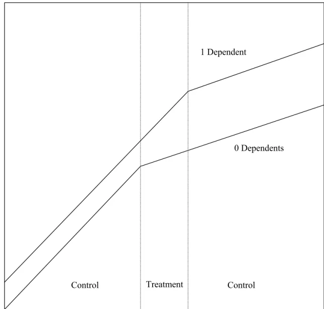
Figure 2 shows the change in the budget set for families losing a dependent in the median
income range. For a given level of income, after tax income shifts down as a result of the loss of the dependent exemption. For some families, this loss does not affect the marginal tax rate. For families with initial income in the region immediately below the kink point, the loss of the dependent exemption shifts them into a higher tax bracket. Given the same level of income, they now face a higher marginal tax rate. As the figure shows, there are no dominated kink points in our experiment; families may rationally chose to locate over the entire budget set.
7Similar changes in the location of the kink point occur at the 28% to 31% bracket for families with income between $118,000 and $128,000. See Looney and Singhal (2004) for a discussion of other provisions in the tax code tied to a child’s age and/or post-secondary school attendance.
Our identification strategy compares changes in labor supply of families for whom the loss of a dependent causes a change in marginal tax rates (the “treatment” group illustrated on Figure 2) to changes of families for whom the loss of a dependent has no marginal tax consequences (the “control” groups). The loss of a dependent may, of course, have a number of direct effects on labor supply. However, as long as these direct effects are the same for treatment and control families, our estimates will not be affected. Under the assumption that treatment and control groups experience similar changes in tastes and shocks to income between periods, the behavioral responses are identified by changes in the tax rate of the treatment group.8
This approach also addresses concerns that differential income trends between treatment and control groups can bias estimates of the response to wage and tax changes (Slemrod 1996, Goolsbee 2000a, 2000b). Our treatment and control groups are very similar and we include controls for base period income. We also test for the possibility of differential income trends in Section 6.2.
4
Data
We implement our empirical strategy using data from the 1990-1996 panels of the Survey of Income and Program Participation (SIPP) and the NBER tax panel from 1987-1990.9 By exploiting both of these data sources, we are able to provide a comprehensive picture of families’ responses to tax incentives. The SIPP data contains detailed information on all family members, allowing us to identify husbands’ and wives’ responses and also to determine whether responses are occurring on participation, hours or other margins. The SIPP also provides a relatively large sample size and the detailed information on children required to predict their status as dependents. The tax panel
8
Although thesefigures illustrate only federal marginal tax rates, our empirical analysis uses the TAXSIM calcu-lators and incorporates state tax rates as well as certain provisions of the child tax credit that can affect marginal tax rates when a child turns 17.
9The tax panel data are also referred to as the University of Michigan Tax Panel and the Continuous Work History File. Note that the short panels of the CPS are not suitable for our analysis because of the difficulty identifying dependents once they leave the household and poor matching rates.
is smaller and contains only the most rudimentary demographic information, but has the advantage of including income measures taken directly from tax forms without measurement error and allows us to capture other dimensions of the behavioral response to taxation. In addition, we are able to test our methodology using two entirely separate data sets.
The SIPP is a nationally representative panel survey of households. Each panel includes between 20,000 and 45,000 households. Within panels each household is interviewed at four month intervals for between 28 and 48 months. The 1990-1996 panels cover the time period from 1990 to 1999. We focus our attention on married couples who live with their own dependent children (children under age 19 or under 24 and full time students) at some point during the panel.10
Our empirical strategy involves looking at year to year changes in income and taxes so we first-difference the annual observations and use these changes as the unit of observation. We retain only those families with first-period income between $35,000 and $85,000 per year. We drop families that experience a change in marital status. Table 1 provides summary statistics for this sub-sample of interest. Column 1 includes all observations. Families averaged $56,430 in earnings (defined as labor income earned by the mother or father). Women in the sample are, on average, 39 years old (husbands are about 2 years older), high school graduates, and have 1.8 dependents living in their household. 11 percent are non-white.
Columns 2 and 3 compare those with no change in the number of dependent children to those that have one fewer because of a change in the age of their child.11 In general, these families are very similar. Mothers losing a dependent are seven years older than those with no change, have slightly lower mean income and schooling, and mechanically have one less child.
We augment these data with the NBER tax panel for the years 1987-1990. The tax panel, 10We limit our sample to married couples because non-married parents often have a choice over which individual claims a child as a dependent. Such claiming decisions may be endogenous to tax incentives.
11
The remaining families included in column 1 are almost entirely families who experienced a gain of one dependent; families experiencing a gain or loss of more than one dependent represent less than 1% of the sample.
assembled by the Statistics of Income Division of the IRS, is a longitudinal sample of federal tax returns sampled randomly on the basis of the last four digits of filers’ social security numbers. These data span the time period from 1979 to 1990. However, we use only the 1987-1990 years to avoid complications associated with the 1981 and 1986 tax reforms and because the tax schedule during this period more closely resembles the schedule we examine in the SIPP data. These data provide excellent information on tax-related variables; almost every element of a typicalfiler’s return is recorded in the data. However, the only demographic information contained in the data is marital status (throughfiling status) and a proxy for children (through number of dependents). The sample originally contained more than 46,000 returns, but after 1981 the IRS choose to follow only a fraction of the original sample. Combined with attrition due to factors like marriage and non-filing, approximately 20,000 returns remain each year between 1987-1990.
Our sample restrictions are similar to those used for the SIPP. We again restrict the sample to married couples and drop returns filed by dependents or irregular filers and those who change filing status.
Table 2, column 1, shows that families in the selected income range have average wage income of $56,272 (in 2000$), almost identical to the SIPP sample. Average adjusted gross income (AGI) is $62,601 and taxable income is $29,913. Filers claim an average of 1.3 dependents. Columns 2 and 3 again compare those losing a dependent to those with no change in the number of dependents. These groups appear quite similar.
5
Methods
The outline of our empirical strategy is as follows: Wefirst predict the change in marginal tax rates faced by families assuming that family income remains constant in real terms between year 1 and year 2. We then instrument for the actual change in the net-of-tax rate with our predicted change
in net-of-tax rate. Regressing changes in labor supply and income variables on this instrumented change in tax price produces estimates of the relevant elasticities.
We estimate the change in marginal tax rates using the NBER TAXSIM program.12 TAXSIM calculates state and federal tax liabilities and tax rates from survey data using information on income, marital status, and number and age of children. For each family, we calculate the predicted tax rate change from year 1 to year 2 as the difference between the log predicted tax price in year 2 and the actual log tax price in year 1, where the prediction is formed using constant real income and actual number of dependents. Formally this corresponds to the following:
d
∆ln(1−τ)it=T axit−1(Incomeit−1, dependentsit)−T axit−1(Incomeit−1, dependentsit−1) (5)
where ∆ln(1d−τ)it is the predicted tax rate change faced by individual i between periods t−1 (year 1) and t (year 2), and T axit−1() is the tax schedule faced individuali in period t−1 as a function of income and number of dependent children. Note that we use thet−1 tax schedule in both years when forming our prediction so that we do not confound changes in tax rates arising from changes in dependents with those arising from changes in tax policy. When using the SIPP data, we define a dependent to be any individual who is eligible to be claimed as a dependent: individuals under 19 living in the household and individuals under 24 who are full-time students.13 In the publicly available tax panel data, we do not have precise information on the ages of children. Therefore, we use changes in dependents claimed as reported on the tax return.
Table 3 provides summary statistics for these tax parameters. In the SIPP sample, families
12
See Feenberg and Coutts (1993) for a detailed explanation of the TAXSIM calculators.
13To test our assignment of dependents, we merge data from SIPP Tax Modules to our sample. The predicted number of dependents matches the actual number recorded by the SIPP 92 percent of the time for people with a copy of their tax form (N=4,844) and 87 percent of the time more generally (N=15,955). Even for children 18 or older, our predictions match actual reported dependents correctly 74 percent of the time. In addition to measurement error, part of the mismatch appears to be due to the fact that 4 percent of married couples reportfiling separately.
who lose a dependent and those who do not appear very similar in year 1: the year 1 marginal tax rate and the average taxes paid in year 1 are 31.6 percent and $11,875 for families with no change and 31.5 percent and $11,845 for families who lose a dependent. Thesefigures include federal, state and FICA taxes. The predicted tax parameters for year 2 are different in the directions we would expect. Families without a change in dependents are predicted to face no change in marginal tax rates and only a $5 increase in tax liability.14 In contrast, families losing a dependent are predicted to experience an increase in marginal tax rates (to 32.3 percent) and an increase in tax liability (to $12,456).15 Columns 3 and 4 present these statistics for the tax panel sample. The year 1 marginal tax rates and average taxes paid are comparable across groups and are similar to those from the SIPP sample. The year 2 predicted marginal tax rate and tax liability are again higher for families losing a dependent than for families with no change.
As a prelude to the estimation strategy described below, we separate the sample of individuals who lose a dependent into those predicted to experience a tax change and those for whom no change is predicted. Table 4Aprovides statistics for the SIPP and tax panel samples. The net of tax rate falls for families experiencing a tax change (by 12 percent on average in the SIPP sample and by 11 percent in the tax panel) as parents are bumped into higher tax brackets as a result of losing exemptions. Those who experienced this decrease in the net of tax rate also experienced a larger drop in income than those with no change in the tax rate. In the SIPP sample, earnings of families with a change in tax rate dropped by $2,082 on average between year 1 and year 2 compared to a decrease of only $79 for families with no change. The same pattern is evident in the tax panel sample: average earnings of families with a tax rate change dropped $3,275 compared to a drop of 14The small change in tax liability for families with no change in dependents arises from families whose taxes are affected by the loss of the child tax credit when children age from 16 to 17. This is only relevant in the last two years of the SIPP sample, and is not relevant in the tax panel sample.
15
The increase in marginal tax rates for this group is small on average because most families losing a dependent do not experience a resulting tax rate change.
$586 for families with no change.
The average drop in log earnings for families experiencing a change in tax rate is 9 percent compared to 4 percent for families with no change in the SIPP sample (Table 4B). The implied elasticity using a differences-in-differences approach is therefore 0.42, significant at the 10 percent level.16 In the tax panel, the average drop in log earnings for families experiencing a tax change is 10 percent, compared to 6 percent for families with no change. The implied elasticity in this sample is 0.36, very similar to the SIPP estimate.17 Our empirical strategy aims to formalize these relationships.
We instrument for the actual change in the log tax price with our predicted change and estimate equations similar to those described in Section 2:
∆ln (lit) =γ∆ln (1−τit) +βXit+εit (6)
where ∆ln (lit) is the change in log labor supply (or income), ∆ln (1−τit) is the instrumented change in the log of the tax price, which measures the change in the net-of-tax wage, and Xit are covariates intended to control for changes in tastes. γ is the estimate of the elasticity of intertemporal substitution.
6
Results
6.1
Elasticity of Family Labor Income
We focus on families shifting from the 15 percent bracket to the 28 percent bracket as the result of losing a dependent exemption. This is likely to be the cleanest experiment since families are 16The implied elasticity is the difference in the log change in earnings between treatment and control divided by the difference in the log change in tax price between treatment and control; in this case, -0.05 divided by -0.12.
17In these differences calculations (as well as in the following analyses), 7 families in the SIPP and 6 families in the tax panel are dropped as a result of having no labor income in the second year.
likely to anticipate the loss of a dependent exemption well in advance. Table 5 presents elasticity estimates from the SIPP sample. The sample in columns 1-3 consists of families with income between $35,000 and $85,000 who lost a dependent between years 1 and 2. Column 1 presents the base IV regression of change in log family earnings on change in log tax price controlling for the log of family earnings in year 1 and yearfixed effects. The elasticity estimate is 0.75 with a standard error of 0.38. This implies that a one percent change in a family’s net-of-tax wage rate results in a 0.75 percent change in family labor earnings.
Adding controls for the number of dependents in year 2 (column 2) and mother’s years of education (column 3) leaves the elasticity estimate virtually unchanged, and the estimates are now significant at the 5% level. The coefficient on log year 1 earnings is negative (around -0.14) as would be expected if families experience mean reversion in earnings. These results are robust to adding additional demographic and base-period income controls as would be expected if treatment and control groups are similar. Controlling for changes in the log of predicted after tax income does not affect the elasticity estimate.
The results are also robust to perturbations of the income range. Using families above the kink as the control group (income range $55-85,000) gives an estimate of 0.89 (column 4). Using families below the kink as the control (income range $35-65,000) gives an estimate of 1.04 (column 5). The point estimate remains stable when the income range is narrowed around the discontinuity (column 6). The standard error increases in columns 5 and 6 as a result of reductions in sample size, but the estimates remain significant at the 10% level.
There are several reasons why our estimates may in fact be lower bounds on the true behavioral response. First, some families may not be aware of the potential change in marginal tax rates arising from changes in dependents. Second, families may not have full control over their incomes. As Saez (2003) points out, this may cause jumps in marginal tax rates to be partially smoothed out,
implying that families’ perceived changes in marginal tax rates may be lower than actual changes. These factors should all create a downward bias in our estimates. Finally, if some families are myopic and do not predict the change in dependents or if families face credit constraints, they may be experiencing income effects. In general, this would also cause us to underestimate the true substitution effect and bias our results towards the uncompensated elasticity of labor supply that would arise from a static model. However, both treatment and control groups would experience similar income effects, minimizing this potential source of bias.
Despite the downward biases mentioned above, these elasticities are significantly higher than those estimated in early studies of intertemporal labor supply and lie at the high end of the most recent estimates of the elasticity of taxable income. If tax changes are anticipated, estimates are not downward biased by income effects. This bias may be quite substantial. In a survey module of the Health and Retirement Study, Kimball and Shapiro (2003) ask respondents to predict their labor supply response to a hypothetical lottery win and use these data to estimate income effects. In their framework, which assumes that income and substitution effects perfectly offset, these estimates imply a substitution elasticity of one, consistent with our estimates.18 Anticipation also means that families have the ability to respond both ex-ante and ex-post, leading to potentially larger measured responses.19
It should be noted that we are comparing only year-to-year changes and therefore capture only short-run responses to taxation. There are two major reasons we might in general expect short-run responses to tax changes to differ from long-run responses. First, families may shift income over time in response to the change, creating an upward bias in the ”true” response. While this has 18The assumption of cancelling income and substitution effects is motivated by estimates of uncompensated elas-ticities close to zero (Pencavel 1986). Imbens, Rubin and Sacerdote (2001)find smaller but still substantial income effects using data from a survey of actual lottery participants.
19
It is also possible that families are especiallyflexible at the time a child leaves the household or completes school, making them particularly responsive to tax incentives.
been raised as a concern in studies of the rich (Slemrod 1995), it is less likely to be a concern for families in our income ranges as they have little capital income. Second, families may face commitments that make it difficult to adjust immediately in response to a tax change. In this case, short-run effects might understate long-run impacts. Again, this is unlikely to be problematic in our case. Because families can anticipate these tax changes in advance, they have time to make necessary adjustments. In this sense, our estimates should be capturing what would traditionally be thought of as the long-run response in a world with commitments. There may, however, be other reasons why short-run and long-run responses differ. Because the SIPP panels are 2 1/2 to 4 years and we are able to use only 4 years of the tax panel, we are limited in our ability to explore the dynamics of the effect over a longer time horizon.
6.2
Placebo Tests
A potential concern with these estimates is that families in income ranges close to and away from the kink may have experienced differential income trends in the absence of a tax rate change. This is unlikely to be a problem since our income range is fairly narrow, treatment and control groups look similar on observables, and we control for base year income. Nevertheless, as a test of our identification strategy we run the following placebo test. We take the sample of families in our income range who did not experience a change in the number of dependents, predict their tax changes as if they had experienced a loss in dependents and examine their income changes. Families with predicted tax changes will be those families close to the kink point, allowing us to test whether our predicted tax change parameter is capturing other characteristics of these families. We also estimate the effects using simulated tax schedules in which the tax rate discontinuity is shifted to alternate levels of income. If our estimates are driven by discontinuous changes in taxes arising from changes in dependents (rather than differential income trends or other spurious effects), we
should find no response for these groups.
Tables 6A and 6B shows the summary statistics using simulated dependent changes. In this
sample, families predicted to experience a tax rate change (those near the kink point) have very similar changes in income to those families predicted to have no change. The difference between the groups is small and insignificant. This placebo test shows that our results do not appear to be driven by families in income ranges near the kink point having different income trends from families in income ranges away from the kink. Restricting the placebo sample to families whose oldest child is between 16 and 18 in year 2 gives similar results.20
We then simulate alternative tax schedules and use our methodology to calculate elasticities under the assumption that the treatment groups faced the simulated schedules (Table 7). In particular, we shift the tax schedule to the left by $5,000 and to the right by $5,000. The resulting elasticity estimates for these simulated tax schedules are not significant.
6.3
Decomposition of the E
ff
ects
The tax rate changes we consider affect marginal tax rates at the family level; the elasticity of family labor income is therefore the measure that best captures the total labor supply response to the change in the net-of-tax wage rate. In this section, we make use of the detailed labor supply data in the SIPP to gain a better understanding of the various components that comprise the total family response. In particular, we examine whether husbands or wives appear to be responding, and whether the response is on participation, hours, or other margins. We run unconditional regressions of change in labor income on change in tax price for husbands and wives separately and similar regressions for changes in participation and hours.
20Running our regression analysis on the sample with simulated dependent changes confirms the results of the summary statistics table (Table 6C). However, the predicted tax change instrument is weak in this case, since these families do not experience actual dependent related tax changes. We therefore consider the summary statistics evidence more compelling.
These coefficients should not be interpreted as individual elasticities because the tax rate changes affect both members of the household. Without making strong assumptions about the interaction of preferences within the household (for example, assuming that the husband’s labor supply is fixed), we cannot recover the underlying elasticities for each individual. These estimates provide information about the composition of the aggregate response but should not be compared to existing estimates of participation and hours elasticities.
Table 8 presents the results for families in the $35-85K range losing a dependent. We observe
an earnings response for both husbands and wives (columns 2 and 3). The responses along participation and hours margins are more mixed. Somewhat surprisingly, the aggregate annual hours response is close to zero (column 4) with the point estimates for wives’ and husbands’ hours (columns 5 and 6) suggesting offsetting increases for wives and declines for men. However, caution should be used when interpreting the hours response because reported hours are clustered at 2,080 and 4,160 hours per year (40 hours per week for 52 weeks per year) suggesting that reported hours may not reflect actual hours. In columns 7 and 8 the dependent variable is a dummy variable indicating the individual has exited the labor force.21 These regressions are intended to examine the participation response. The point estimates suggest that higher net-of-tax wages are associated with a higher probability of leaving the labor force (for women) and a lower probability for men, but the estimates are statistically not significant.
Note that there may be variation in the change in labor earnings that is not captured by partic-ipation and hours or not reflected because of reporting errors in measured hours or particpartic-ipation. Changes in family labor earnings may also reflect changes in effort or shifts between wage and non-wage compensation.
21The sample of individuals not in the labor force is too small to estimate the probability of entering the labor force.
6.4
Estimates for the EITC Range
We now examine the response to dependent related tax changes for families in other parts of the income distribution. We focus in particular on families in the phaseout region of the EITC, restricting the sample to families with base year income between $10,000 and $40,000 (Table 9). We estimate an elasticity of family labor income for families losing a dependent of 0.14 (not significant).
The downward bias caused by families not understanding the tax rate implications of a depen-dent change may be severe for this group, particularly since we measure thefirst year response. As shown in Figure 1, these families are shifted from one complex tax schedule to another as a result of dependent changes. It is possible that these families do respond once the change is understood, but we are not able to examine this with the short panels available in our data. It may also be the case, however, that the difference between the EITC and middle-income group responses is a result of true heterogeneity in elasticities over the income distribution.
Due to sample size constraints, we are unfortunately not able to estimate stable responses for higher income groups.
6.5
Estimates from the Tax Panel
We now use our methodology to estimate behavioral responses in the IRS-NBER tax panel. This allows us to test our methodology and compare elasticity estimates using a data set entirely un-related to the SIPP data. In addition, using tax panel data we can estimate elasticities of AGI and taxable income. The elasticity of taxable income captures the full behavioral response to the tax rate change and, as emphasized by Feldstein (1999), is the relevant parameter for evaluating the efficiency costs of taxation. We focus on the $35,000-$85,000 income range because sample sizes other income ranges are too small to estimate stable elasticities.22 We construct the sample 22Note that this is entirely due to data constraints; our methodology could be used to provide estimates for these income ranges with richer data.
as described in Section 3 and assign returns taxable income of $1 if they report no taxable income and AGI is positive.
Table 10 presents these results. Columns 1-3 present the elasticity estimates of wage income,
AGI and taxable income. The elasticity estimate for wage income is 0.71, almost identical to the SIPP estimate of 0.75. The point estimates of the elasticities of AGI and taxable income are 0.54 and 3.2 respectively. The estimates are not statistically significant, however, which is perhaps not surprising given the smaller sample sizes in the tax panel. Nevertheless, the point estimates indicate substantial elasticities that are quite consistent with the SIPP estimates.
We then define the sample income range by initial taxable income, rather than earnings. The bracket kink occurs between $40,000 and $50,000 of taxable income, so we restrict the sample to those families whose base year taxable income is between $20,000 and $70,000.23 We find very similar results for the elasticity of wage income: the point estimate is 0.73 (column 4). The estimates for AGI and taxable income are 0.04 and 1.07, but the standard errors are very large.
As most of the empirical literature on taxable income elasticities does not distinguish between life-cycle wealth effects and static income effects, our estimates can be compared to the compensated elasticities estimated in the tax literature and interpreted similarly.24 For example, Saez (2003) and Gruber and Saez (2002), interpret their estimates as compensated elasticities. In this context, our preferred estimates from both the SIPP and Tax Panel (an elasticity of .7) lie at the high end of the range of recent estimates of the elasticity of taxable income, and therefore imply significant 23The location of the bracket kink point technically depends on taxable income. These data are not available in the SIPP. The standard deduction for married couplesfiling jointly plus two personal exemptions is about $15,000 in 2000.
24In a strict structural framework, our estimated elasticities are intertemporal (marginal utility of wealth constant) elasticities. Intuitively, intertemporal elasticities measure responses to movements along a wage profile, holding the marginal utility of wealth constant, and compensated elasticites measure responses to shifts of the wage profile, holding lifetime utility constant. MaCurdy (1981) shows that the Hicksian (compensated) labor supply elasticity is bounded above by the intertemporal elasticity and below by the uncompensated elasticity. Our estimates could therefore be considered to be upper bounds on the compensated elasticity.
behavioral responses to taxation and sizable efficiency costs of taxation.
7
Conclusion
Our empirical strategy employs anticipated changes in marginal tax rates arising from changes in dependents to estimate the behavioral response to taxation. This strategy has certain advantages over strategies that examine the response to legislated changes in tax policy. Most importantly, the tax rate changes we study are fully anticipated and should induce no income effects. Therefore, we can interpret our estimates to be pure substitution elasticities. One reason why our estimates fall on the high side of conventional estimates may be because estimates of substitution elasticities from static models confound life-cycle wealth effects with intertemporal substitution effects.
The intertemporal elasticity of labor supply has important implications for understanding ag-gregate employment and output fluctuations. If workers respond to changes in wages over time by reallocating labor across periods, then productivity shocks can generate large cyclical fluctua-tions (Prescott 1986a). One of the central quesfluctua-tions in the debate about these real business cycle models is whether the magnitude of intertemporal substitution is large enough to explain fluctua-tions of the size we observe in the United States economy. Our high-end estimates are consistent with the range of elasticities implied by calibration of real business cycle models to the data on macroeconomicfluctuations.25
Most of our estimates of taxable income elasticities are unfortunately imprecise as a result of data limitations. In theory, however, our estimates of labor income elasticities from the SIPP data should be lower bounds on the true elasticities of taxable income. The high-end estimates then imply substantial behavioral responses to taxation.
25There are other points of contention between proponents and opponents of real business cycle models. See Summers (1986), and Mankiw (1989) for discussion.
Exploiting child-related tax rate changes provides a consistent identification strategy for esti-mating elasticities across the income distribution and over different periods of time. There is no reason to expect a constant elasticity across income groups, and understanding elasticity hetero-geneity is critical for the design of optimal tax systems. In addition, diffusion of asset ownership, changes in tax law and changes in tax enforcement might all affect the ability of individuals to respond to tax incentives. As Slemrod (1998) and others have pointed out, it is unclear whether differing elasticity estimates in the literature are a result of differences in methodology, differential biases across policy experiments, or differences in behavioral responses at different points in time. We believe that this method has great promise for identifying true heterogeneity in elasticities across different income groups as well potential changes in these elasticities over time.
References
[1] Altonji, Joseph. ”Intertemporal Substitution in Labor Supply: Evidence from Micro Data.” Journal of Political Economy. 94(3): S176-S215, 1986.
[2] Auten, Gerald and Robert Carroll. ”The Effect of Income Taxes on Household Behavior.” Review of Economics and Statistics. 81: 681-93, November 1999.
[3] Blomquist, N. Soren. ”Labor Supply in a Two-Period Model: The Effect of a Nonlinear Progressive Income Tax.” The Review of Economic Studies. 52: 515-524, 1985.
[4] Blundell, Richard and Thomas MaCurdy. ”Labor Supply: A Review of Alternative Ap-proaches,” in Handbook of Labor Economics, vol. 3, O. Ashenfelter and D. Card, eds. Amsterdam: Elsavier, 1999.
[5] Card, David. ”Intertemporal Labor Supply: An Assessment,” in Advances in Econometrics, C.A. Sims, ed. Sixth World Congress, 1994.
[6] Eissa, Nada. ”Taxation and Labor Supply of Married Women: The Tax Reform act of 1986 as a Natural Experiment.” NBER Working Paper 5023, February 1995.
[7] Dokko, Jane K. ”The Effect of Taxation on Lifecycle Labor Supply: Results from a Quasi-Experiment.” mimeo, University of Michigan, 2005.
[8] Eissa, Nada and Hilary Hoynes. ”The Earned Income Tax Credit and the Labor Supply of Married Couples.” NBER Working Paper 6856, December 1998.
[9] Eissa, Nada and Jeffrey Leibman. ”Labor Supply Responses to the Earned Income Tax Credit.” Quarterly Journal of Economics. 111: 605-637.
[10] Feenberg, Daniel and Elizabeth Coutts. ”An Introduction to the TAXSIM Model.” Journal of Policy Analysis and Management. 12(1): 189-194, 1993.
[11] Feldman, Naomi and Peter Katuscak. ”Should the Average Tax Rate Be Marginalized?” mimeo, UCSD, 2005.
[12] Feldstein, Martin. ”The Effect of Marginal Tax Rates on Taxable Income: A Panel Study of the 1986 Tax Reform Act.” Journal of Political Economy. 103(3): 551-572, 1995.
[13] Feldstein, Martin. ”Tax Avoidance and the Deadweight Loss of the Income Tax.” The Review of Economics and Statistics. 81(4): 674-680, November 1999.
[14] Feldstein, Martin. ”The Effect of Marginal Tax Rates on Taxable Income: A Panel Study of the 1986 Tax Reform Act.” Journal of Political Economy. 103(3): 551-572, June 1995. [15] Giertz, Seth. ”Recent Literature on Taxable-Income Elasticities.” CBO Technical Paper Series
2004-16, December 2004.
[16] Goolsbee, Austan. ”It’s Not About the Money: Why Natural Experiments Don’t Work on the Rich,” inDoes Atlas Shrug? The Economic Consequences of Taxing the Rich, J. Slemrod Ed. Cambridge: Cambridge University Press, 2000b.
[17] Goolsbee, Austan. ”What Happens When You Tax the Rich? Evidence from Executive Compensation.” Journal of Political Economy. 108(2): 352-378, 2000b.
[18] Gruber, Jonathan and Emmanuel Saez. ”The Elasticity of Taxable Income: Evidence and Implications.” Journal of Public Economics. 84:1-32, 2002.
[19] Heckman, James and Mark R. Killingsworth. ”Female Labor Supply: A Survey,” inHandbook of Labor Economics, vol. 1, O. Ashenfelter and R. Layard, eds. Amsterdam: North Holland, 1986.
[20] Imbens, Guido W., Donald B. Rubin and Bruce Sacerdote. ”Estimating the Effect of Unearned Income on Labor Supply, Earnings, Savings and Consumption: Evidence from a Survey of Lottery Players.” American Economic Review. 91(4): 778-794, 2001.
[21] Kimball, Miles S. and Matthew D. Shapiro. ”Labor Supply: Are the Income and Substitution Effects Both Large or Both Small?” mimeo, University of Michigan, 2003.
[22] Kopczuk, Wojciech. ”Tax Bases, Tax Rates and the Elasticity of Reported Income.” Journal
of Public Economics. 89:2093-2119, 2005.
[23] Looney, Adam and Monica Singhal. ”Family Composition and Marginal Tax Rates: An Identification Strategy for Estimating Intertemporal Labor Supply Substitution.” National Tax Association Proceedings, 2004.
[24] MaCurdy, Thomas. ”An Empirical Model of Labor Supply in a Life Cycle Setting.” Journal of Political Economy. 88(6): 1059-85, 1981.
[25] Mankiw, Gregory. ”Real Business Cycles: A New Keynesian Perspective.” The Journal of Economic Perspectives. 3(3): 79-90, Summer 1989.
[26] Meyer, Bruce. ”Labor Supply at the Extensive and Intensive Margins: The EITC, Welfare and Hours Worked.” American Economic Review. 92: 373-379, 2002.
[27] Meyer, Bruce and Daniel Rosenbaum. ”Welfare, the Earned Income Tax Credit, and the Labor Supply of Single Mothers.” Quarterly Journal of Economics. 116(3): 1063-1113, 2001. [28] Mulligan, Casey. ”Substitution Over Time: Another Look at Life Cycle Labor Supply.” NBER
Working Paper 6585, May 1998.
[29] Mroz, Thomas. ”The Sensitivity of an Empirical Model of Women’s Hours of Work to Eco-nomic and Statistical Assumptions.” Econometrica. 55: 765-799, 1987.
[30] Pencavel, John. ”Labor Supply of Men: A Survey,” inHandbook of Labor Economics, vol. 1, O. Ashenfelter and R. Layard, eds. Amsterdam: North Holland, 1986.
[31] Prescott, Edward. ”Theory Ahead of Business Cycle Measurement.” Carnegie-Rochester Conference on Public Policy. 25: 11-44, Autumn 1986a.
[32] Saez, Emmanuel. ”The Effects of Marginal Tax Rates on Income: A Panel Study of ‘Bracket Creep.’” Journal of Public Economics. 87:1231-1258, 2003.
[33] Slemrod, Joel. ”Income Creation or Income Shifting? Behavioral Responses to the Tax Reform Act of 1986.” American Economic Review. 85:175-180, May 1995.
[34] Slemrod, Joel. ”Methodological Issues in Measuring and Interpreting Taxable Income Elas-ticities.” National Tax Journal. 51(4): 773-788, December 1998.
[35] Slemrod, Joel. ”High Income Families and the Tax Changes of the 1980s: The Anatomy of Behavioral Response,” inEmpirical Foundations of Household Taxation, M. Feldstein and J. Poterba, Eds. Chicago: University of Chicago Press, 1996.
[36] Summers, Lawrence H. ”Some Skeptical Observations on Real Business Cycle Theory.” Federal Reserve Bank of Minneapolis Quarterly Review. 10(4): 9-22, Fall 1986.
[37] Ziliak, James P. and Thomas J. Kniesner. ”Estimating Life Cycle Labor Supply Tax Effects.” Journal of Political Economy. 107(2): 326-359, 1999.
Data Appendix
This paper uses data from the 1990, 1991, 1992, 1993, and 1996 panels of the Survey of In-come and Program Participation. The SIPP is a nationally representative longitudinal sample of American households and contains monthly observations over a period of 28 to 48 months.
The data is processed as follows. The sample is first restricted to married couples for whom income data is available for both husband and wife. Wage, property income, and employment data are annualized. Occasionally one or more months of income data is missing; the average values from non-missing months is imputed for those months but couples observed for fewer than 9 months in a single year are dropped. (Missing observations arise largely because of marriage or divorce during the year, the timing of interviews during the calendar, and sample attrition.)
For each couple, we calculate the number of dependent children as the number of own children living in their household (or away at school) as of December (or the last month the couple is observed in the sample, if December is missing) of each year who are under age 19 or under age 24 and a full-time student. Couples with no dependent children at any point throughout the panel are dropped. Observations where the age difference between mother and children are unusually large or small (less than 15 years or more than 40 years) are dropped.
In addition, we use data from the continuous work history sample or IRS/NBER tax panel. We focus on the years from 1987 to 1990 and again retain taxpayers filing as Married Filing Jointly. Income variables, dependent exemptions,filing status, and deductions are included in the data.
Tax rate variables are calculated using NBER Taxsim. This program takes income and other variables, including state, year, wages, property income, marital status, number of dependents, and other variables and produces estimated marginal tax rates. The instrumented marginal tax rate change between period t and t+1 is calculated by re-estimating marginal tax rates using the demographic information for period t+1 but the income and other variables as of period t. We use the period t tax schedule as well to avoid confounding our estimates with responses caused by changes in policy.
-40
-30
-20
-10
0
10
20
30
40
Marginal Tax Rate
0
1000
0
2000
0
3000
0
4000
0
5000
0
6000
0
7000
0
8000
0
9000
0
10
000
0
11
000
0
12
000
0
13
000
0
14
000
0
15
000
0
Annual Income
No Children
1 Child
2 Children
3 Children
Source: Authors calculations using NBER Taxsim assuming joint filing status, wage income, taking the
standard deduction.
Federal Marginal Tax Rates by AGI and Number of Dependents (2000)
Figure 1
Figure 2: The Effect of a Change in Dependents on Marginal Tax Rates
Treatment
1 Dependent
0 Dependents
Control
Control
After Tax In
come
Income range: $35-85K
All
No change in
1 less dependent
# dependents
Family earnings
56430
56682
55540
(20718)
(20717)
(21869)
Age of mother
38.8
38.8
45.4
(7.8)
(7.5)
(6.0)
Age of father
41.0
41.1
47.8
(8.3)
(8.0)
(6.7)
Non-white (mother)
.11
0.11
0.12
(0.31)
(0.31)
(0.32)
Years of school (mother)
13.1
13.1
12.6
(1.7)
(1.7)
(1.8)
# Year 2 dependents
1.75
1.79
0.97
(1.06)
(1.03)
(1.04)
Observations
30367
25848
1947
Notes: Data: 1990-1996 SIPP panels. Includes married couples with children living in their home with income between $35,000 and $85,000. See text for details. Family earnings refers to labor income earned by the mother and father. Standard deviations in parentheses. Dollar figures adjusted to 2000$ using the CPI-U.
Table 1
Income range: $35-85K
All
No change in
1 less dependent
# dependents
Family earnings
56272
56395
56699
(20097)
(19335)
(30451)
AGI
62601
62493
67022
(41097)
(33257)
(102365)
Taxable Income
29913
30056
32231
(22402)
(20772)
(38591)
# Year 2 dependents
1.30
1.26
1.02
(1.21)
(1.20)
(1.14)
Observations
11733
10011
740
Notes: Data: Tax Panel 1987-1990. Includes married couples with children living in their home with wage income between $35,000 and $85,000. See text for details. Standard deviations in parentheses. Dollar figures adjusted to 2000$ using the CPI-U.
Table 2
No change in
1 less
No change in
1 less
# dependents
dependent
# dependents
dependent
Marginal tax rate (year 1)
31.6
31.5
31.6
31.7
(7.1)
(7.1)
(7.3)
(7.8)
Predicted MTR (year 2)
31.6
32.3
31.6
32.4
(7.1)
(7.3)
(7.3)
(7.9)
Taxes paid (year 1)
11875
11845
12380
13130
(4676)
(4743)
(8208)
(19259)
Predicted taxes (year 2)
11880
12456
12380
13742
(4675)
(4890)
(8208)
(19275)
Observations
25848
1947
10011
740
Notes: Source: 1990-1996 SIPP Panels and NBER Tax Panel 1987-1990. Tax parameters calculated using TAXSIM. Standard deviations in parentheses.
Table 3
Predicted Tax Parameters
No change in
Change in
No change in
Change in
tax rate
tax rate
tax rate
tax rate
Panel A: Changes in Marginal Tax Rates
Marginal tax rate (year 1)
31.8
28.4
32.1
28.3
(7.2)
(4.5)
(7.9)
(6.5)
Predicted MTR (year 2)
31.8
36.6
32.1
35.7
(7.2)
(6.1)
(7.9)
(7.6)
Δ
ln(1-
τ
) (predicted)
0
-0.12
0
-0.11
(0.09)
(0.10)
Panel B: Changes in Earnings
Earnings (year 1)
55811
55729
57733
56056
(13999)
(9920)
(14102)
(12927)
Earnings (year 2)
55732
53647
57147
52781
(22374)
(15965)
(31500)
(18643)
Δ
ln(earnings)
-0.04
-0.09
-0.06
-0.10
(0.33)
(0.43)
(0.39)
(0.33)
Difference
Δ
ln(earnings)
(Standard Error)
Observations
1768
179
664
76
Notes: Source: 1990-1996 SIPP Panels and NBER Tax Panel 1987-1990. Tax parameters calculated using TAXSIM. Standard deviations in parentheses. +Denotes statistically significant difference at 10% level.
Table 4
Comparison of means: Families losing a dependent
SIPP
Tax Panel
-0.05
(.027)+
-0.04
(1)
(2)
(3)
(4)
(5)
(6)
Δ
ln(1-
τ
)
0.748
0.754
0.747
0.891
1.040
1.034
(0.383)+
(0.384)*
(0.381)*
(0.408)*
(0.535)+
(0.549)+
ln(year 1 fam labor inc)
-0.142
-0.137
-0.182
-0.317
-0.157
-1.266
(0.050)** (0.049)** (0.052)**
(0.133)*
(0.066)*
(0.627)*
# year 2 dependents
0.022
0.021
0.048
0.020
0.065
(0.009)*
(0.009)*
(0.015)**
(0.012)+
(0.027)*
Years of Education
0.022
0.022
0.024
0.022
(0.005)**
(0.008)** (0.006)**
(0.014)
Year dummies
yes
yes
yes
yes
yes
yes
Constant
1.489
1.410
1.626
3.120
1.337
13.525
(0.544)** (0.534)** (0.541)**
(1.447)*
(0.695)+
(6.851)*
Observations
1940
1940
1940
935
1416
411
Notes: Data: 1990-1996 SIPP panels. The sample consists of married couples who lost a dependent exemption between years 1 and 2. Columns 1-3 include all families with income between $35,000 and $85,000. The sample in column 4 is restricted to those families earning between $55,000 and $85,000. Column 5 is restricted to those earning between $35,000 and $65,000. Column 6 is restricted to those earning between $55,000 and $65,000. Results are robust to richer controls for base year income and demographic characteristics. Robust standard errors in parentheses. + significant at 10%; * significant at 5%; ** significant at 1%.
Table 5
Elasticity Estimates of Family Labor Income (SIPP) (IV)
No change in Change in tax rate tax rate
Panel A: Changes in Marginal Tax Rates
Marginal tax rate (year 1) 31.8 28.3 (7.2) (4.7) Predicted MTR (year 2) 31.8 36.4 (7.2) (5.8)
Δln(1-τ) (predicted) 0 -0.12 (0.09)
Panel B: Changes in Earnings
Earnings (year 1) 55914 55255 (13895) (9782) Earnings (year 2) 56999 55984 (20848) (19562) Δln(earnings) -0.01 -0.02 (0.29) (0.30) Difference Δln(earnings) (Standard Error) Observations 21,197 2,289
Panel C: Placebo Regressions Using Simulated Dependent Changes (IV)
(1) (2)
Δln(1-τ) 0.018 0.002
(0.085) (0.084) ln(year 1 fam labor inc) -0.061 -0.093 (0.011)** (0.012)** # year 2 dependents 0.002
(0.002)
Years of School 0.018
(0.001)**
Year dummies yes yes
Constant 0.615 0.725
(0.120)** (0.120)**
Observations 23468 23468
-0.008
(0.006)
Notes: Source: 1990-1996 SIPP Panels. Tax parameters calculated using TAXSIM. Standard deviations in parentheses (Panels A and B); robust standard errors in parentheses (Panel C). + significant at 10%; * significant at 5%; ** significant at 1%.
Table 6
Comparison of means: Simulated Change in Dependents (Placebo)
+$5,000
-$5,000
(1)
(2)
Δ
ln(1-
τ
)
-0.065
0.304
(0.299)
(0.337)
ln(year 1 fam labor inc)
-0.064
-0.091
(0.042)
(0.040)*
# year 2 dependents
0.013
0.015
(0.008)+
(0.008)+
Year dummies
yes
yes
Constant
0.624
0.917
(0.458)
(0.441)*
Observations
1940
1940
Notes: Data: 1990-1996 SIPP panels. Includes all married couples who lost a dependent exemption between years 1 and 2 and had income between $35,000 and $85,000. Columns 1-2 perturb the tax schedule (and the kink points) up and down by $5,000. Robust standard errors in parentheses. + significant at 10%; * significant at 5%; ** significant at 1%.
Table 7
Tests of the Identification Strategy Using Simulated Tax Schedule
(1)
(2)
(3)
(4)
(5)
(6)
(7)
(8)
Dependent Variable:
Total
Wife
Husband
Total
Wife
Husband
Wife
Husband
Δ
ln(1-
τ
)
0.747
0.360
0.411
0.006
0.179
-0.093
0.251
-0.202
(0.381)*
(0.665)
(0.464)
(0.242)
(0.503)
(0.313)
(0.192)
(0.125)
ln(Lag Earnings,Hours)
-0.182
-0.280
-0.162
-0.125
-0.295
-0.421
(0.052)**
(0.018)**
(0.030)**
(0.018)**
(0.020)**
(0.024)**
# year 2 dependents
0.021
-0.007
0.033
0.009
-0.002
0.005
0.006
-0.005
(0.009)*
(0.015)
(0.012)**
(0.006)
(0.012)
(0.007)
(0.005)
(0.003)
Years of School
0.022
0.033
0.025
0.006
0.009
0.008
0.003
-0.001
(0.005)**
(0.008)**
(0.006)**
(0.003)*
(0.006)
(0.004)*
(0.002)
(0.001)
Year dummies
yes
yes
yes
yes
yes
yes
yes
yes
Constant
1.626
2.302
1.279
0.906
2.050
3.074
0.008
0.011
(0.541)**
(0.195)**
(0.312)**
(0.154)**
(0.170)**
(0.192)**
(0.032)
(0.019)
Observations
1940
1611
1891
1940
1656
1907
1708
1930
Notes: 1990-1996 SIPP panels. Robust standard errors in parentheses. The samples in columns (2), (3), (5), (5), and (6) are for those individuals who did not change their participation decision. The sample in columns (7) and (8) are for those individuals who participated in the labor force in the base year.
Decomposition of the Effects
Table 8
(1)
lose a dependent
Δ
ln(1-
τ
)
0.136
(0.174)
ln(year 1 wage inc)
-0.083
(0.043)+
Year dummies
yes
Constant
0.773
(0.435)+
Observations
1228
Notes: Data: 1990-1996 SIPP panels. The sample consists of married couples who lost a dependent exemption between years 1 and 2 and had income between $10,000 and $40,000. Results are robust to richer controls for base year income and demographic characteristics. Robust standard errors in parentheses. + significant at 10%; * significant at 5%; ** significant at 1%.