Exploring MapReduce Efficiency with
Highly-Distributed Data
∗Michael Cardosa, Chenyu Wang, Anshuman Nangia, Abhishek Chandra, Jon Weissman
University of Minnesota Minneapolis, MN, USA
{cardosa,chwang,nangia,chandra,jon}@cs.umn.edu
ABSTRACT
MapReduce is a highly-popular paradigm for high-performance com-puting over large data sets in large-scale platforms. However, when the source data is widely distributed and the computing platform is also distributed, e.g. data is collected in separate data center loca-tions, the most efficient architecture for running Hadoop jobs over the entire data set becomes non-trivial. In this paper, we show the traditional single-cluster MapReduce setup may not be suitable for situations when data and compute resources are widely distributed. Further, we provide recommendations for alternative (and even hi-erarchical) distributed MapReduce setup configurations, depending on the workload and data set.
Categories and Subject Descriptors
D.4.7 [Organization and Design]: Distributed Systems
General Terms
Management, Performance
1.
INTRODUCTION
MapReduce, and specifically Hadoop, has emerged as a domi-nant paradigm for high-performance computing over large data sets in large-scale platforms. Fueling this growth is the emergence of cloud computing and services such as Amazon EC2 [2] and Ama-zon Elastic MapReduce [1]. Traditionally, MapReduce has been deployed over local clusters or tightly-coupled cloud resources with one centralized data source.
However, this traditional MapReduce deployment becomes in-efficient when source data along with the computing platform is widely (or even partially) distributed. Applications such as scien-tific applications, weather forecasting, click-stream analysis, web crawling, and social networking applications could have several distributed data sources, i.e., large-scale data could be collected in separate data center locations or even across the Internet. For
∗This work was supported by NSF Grant IIS-0916425 and NSF
Grant CNS-0643505.
Permission to make digital or hard copies of all or part of this work for personal or classroom use is granted without fee provided that copies are not made or distributed for profit or commercial advantage and that copies bear this notice and the full citation on the first page. To copy otherwise, to republish, to post on servers or to redistribute to lists, requires prior specific permission and/or a fee.
MapReduce’11, June 8, 2011, San Jose, California, USA.
Copyright 2011 ACM 978-1-4503-0700-0/11/06 ...$10.00.
these applications, usually there also exist distributed computing resources, e.g. multiple data centers. In these cases, the most effi-cient architecture for running MapReduce jobs over the entire data set becomes non-trivial.
One possible “local” approach is to collect the distributed data into a centralized location from which the MapReduce cluster would be based. This would revert into a tightly-coupled environment for which MapReduce was originally intended. However, large-scale wide-area data transfer costs can be high, so it may not be ideal to move all the source data to one location, especially if compute resources are also distributed.
Another approach would be a “global” MapReduce cluster de-ployed over all wide-area resources to process the data over a large pool of global resources. However, in a loosely-coupled system, runtime costs could be large in the MapReduce shuffle and reduce phases where potentially large amounts of intermediate data could be moved around the wide-area system.
A third potential distributed solution is to set up multiple MapRe-duce clusters in different locales and then combine their respective results in a second-level MapReduce (or reduce-only) job. This would potentially avoid the drawbacks of the first two approaches by distributing the computation such that the required data move-ment would be minimized through the coupling of computational resources with nearby data in the wide-area system. One impor-tant issue with this setup, however, is that the final second-level MapReduce job can only complete after all first-level MapReduce jobs have completed, so a single straggling MapReduce cluster may delay the entire computation an undesirable amount.
Important considerations in the above approaches to construct an appropriate MapReduce architecture are the workload and data flow patterns. Workloads that have a high level of aggregation (e.g., Word Count on English text) may benefit largely from a distributed approach to avoid shuffling large amounts of input data around the system when the output will be much smaller. However, workloads with low aggregation (e.g., sort) may perform better under local or global architectures.
In this paper, we show the traditional single-cluster MapReduce setup may not suitable for situations when data and compute re-sources are widely distributed. We examine three main MapReduce architectures given the distributed data and resources assumption, and evaluate their performance over several workloads. We uti-lize two platforms: PlanetLab, for Internet-scale environments, and Amazon EC2 for datacenter-scale infrastructures. Further, we pro-vide recommendations for alternative (and even hierarchical) dis-tributed MapReduce setup configurations, depending on the work-load and data set.
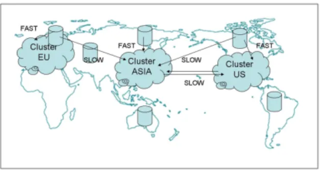
Figure 1: Data and compute resources are widely-distributed and have varying interconnection link speeds.
2.
SYSTEM MODEL AND ENVIRONMENT
2.1
Resource and Workload Assumptions
In our system, we assume we have a number of widely-distributed compute resources (i.e. compute clusters) and data sources. We also have a MapReduce job which must be executed over all the combined data. The following are the assumptions we make in our system model:
• Compute resources: Multiple clusters exist where a cluster
is defined as a local grouping of one or more physical ma-chines. where the machines within the cluster are tightly-coupled. Machines belonging to different clusters are as-sumed to be loosely-coupled. For example, as seen in Fig-ure 1, there could be a compute cluster in the US, one in Europe, and one in Asia.
• Data sources: There exist data sources from various
loca-tions, where large-scale data is either collected or generated. In our example in Figure 1, data sources are shown along with their connection speeds with the compute resources. The bandwidth available between the data sources and com-pute resources is a function of network proximity/topology. In our experiments, we locate data sources within the same clusters as the compute resources.
• Workload: A MapReduce job is to be executed whose
in-put is all the data sources. We explicitly use Hadoop, and assume a Hadoop Distributed File System (HDFS) instanti-ation must be used to complete the job. Therefore the data must be moved from the data sources into HDFS before the job can begin.
2.2
MapReduce Dataflow in Distributed
En-vironments
As previous work in MapReduce has not included performance analysis over wide-area distributed systems, it is important to un-derstand where performance bottlenecks may reside in the dataflow of a MapReduce job in such environments.
Figure 2 shows the general dataflow of a MapReduce job. Prior to the job starting, the delay in starting the job is in the transfer of all data into HDFS (with a given replication factor). If the source data is replicated to distant locations, this could introduce significant delays.
After the job starts, the individual Map tasks are usually executed on machines which have already stored the HDFS data block cor-responding to the Map task; these are normal, “block-local” tasks. This stage does not rely on network bandwidth or latency.
Figure 2: In the traditional MapReduce workflow, Map tasks operate on local blocks, but intermediate data transfer during the Reduce phase is an all-to-all operation.
If a node becomes idle during the Map phase, it may be assigned a Map task for which it does not have the data block locally stored; it would then need to download that block from another HDFS data location, which could be costly depending on which data source it chooses for the download.
Finally, and most importantly, is the Reduce phase. The Reduce operation is an all-to-all transmission of intermediate data between the Map task output data and Reduce tasks. If there is a significant amount of intermediate data, this all-to-all communication could be costly depending on the bandwidth of each end-to-end link.
In the next section, we will propose architectures in order to avoid these potential performance bottlenecks when performing MapRe-duce jobs in distributed environments.
3.
FACTORS IMPACTING MAPREDUCE
PER-FORMANCE
In this section, we study factors that could impact MapReduce performance in loosely-coupled distributed environments. First, we suggest some potential architectures for deploying MapReduce clusters, and then later discuss how different workloads may also impact the performance.
3.1
Architectural Approaches
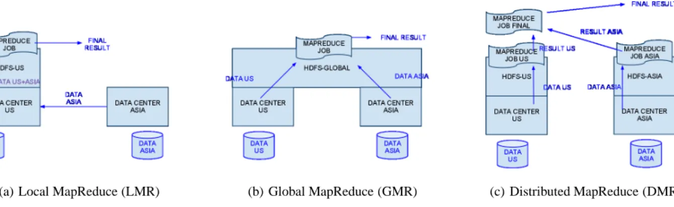
Intuitively, there are three ways to tackle MapReduce jobs run-ning on widely-distributed data. We now describe these three ar-chitectures, showing examples of these respective architectures in Figure 3.
• Local MapReduce (LMR): Move all the data into one
cen-tralized cluster and perform the computation as a local MapRe-duce job in that single cluster itself. (Figure 3(a))
• Global MapReduce (GMR): Build a global MapReduce
clus-ter using nodes from all locations. We must push data into a global HDFS from different locations and run the MapRe-duce job over these global compute resources. (Figure 3(b))
• Distributed MapReduce (DMR): Construct multiple
MapRe-duce clusters using a partitioning heuristic (e.g., node-to-data proximity), partitioning the source data appropriately, run MapReduce jobs in each cluster and then combine the re-sults with a final MapReduce job. This can also be thought of as a hierarchical MapReduce overlay. (Figure 3(c))
(a) Local MapReduce (LMR) (b) Global MapReduce (GMR) (c) Distributed MapReduce (DMR)
Figure 3: Architectural approaches for constructing MapReduce clusters to process highly-distributed data. This example assumes there are two widely-separated data centers (US and Asia) but tightly-coupled nodes inside the respective data centers.
The choice of architecture is paramount in ultimately determin-ing the performance of the MapReduce job. Such a choice depends on the network topology of the system, inter-node bandwidth and latency, the workload type, and the amount of data aggregation oc-curring within the workload. Our goal in this paper is to provide recommendations for which architecture to use, given these vari-ables as inputs.
Next, we examine three different levels of data aggregation oc-curring in different example workloads, from which we will derive our experimental setup for evaluation.
3.2
Impact of Data Aggregation
The amount of data that flows through the system in order for the MapReduce job to complete successfully is a key parameter in our evaluations. We will use three different workload data aggregation schemes in our evaluation, described as follows:
• High Aggregation: The MapReduce output is multiple
or-ders of magnitude smaller than the input, e.g. Wordcount on English plain-text.
• Zero Aggregation: The MapReduce output is the same size
as the input, e.g. the Sort workload.
• Ballooning Data: The MapReduce output is larger than the
input, e.g. document format conversion from LaTeX to PDF.
The size of output data is important because during the reduce phase, the all-to-all intermediate data shuffle may result in consid-erable overhead in cases where the compute facilities have band-width bottlenecks. In our evaluation we will analyze the the perfor-mance of each of the three architectures in combination with these workload data aggregation schemes in order to reach a better un-derstanding of which architecture should be recommended under varying circumstances.
4.
EXPERIMENTAL SETUP
In this section we describe our specific experimental setups over two platforms:
• PlanetLab: A planetary-scale highly-heterogeneous distributed
shared virtualized environment where slices are guaranteed only 1
n of machine resources wherenis the number of
ac-tive slices on the machine. This environment models highly-distributed loosely-coupled systems in general for our study.
• Amazon EC2: The Amazon Elastic Compute Cloud is a
large pool of resources with strong resource guarantees in a large virtualized data center environment. We run exper-iments across multiple EC2 data centers to model environ-ments where data is generated at multiple data center loca-tions and where clusters are tightly coupled.
We use Hadoop 0.20.1 over these platforms for our experiments. In our experimental setups, due to the relatively low overhead of the master processes (i.e., JobTracker and NameNode) given our work-loads, we also couple a slave node with a master node. In all our experiments, source data must first be pushed into an appropriate HDFS before the MapReduce job starts.
We have three main experiments we use in both of our plat-forms for evaluation, involving Wordcount and Sort, and the two different source data types. The experimental setups can be seen in Tables 3 and 5. These experiments are meant to model the high-aggregation, zero-high-aggregation, and ballooning workload dataflow models as mentioned in Section 3.2.
4.1
PlanetLab
In PlanetLab we used a total of 8 nodes in two widely-separated clusters – 4 nodes in the US, 4 nodes in Europe. In addition, we used one node in both clusters as our data sources. For each cluster, we chose tightly-coupled machines with high inter-node bandwidth (i.e., they were either co-located at the same site or share some network infrastructure). In the presence of bandwidth limitations in PlanetLab and workload interference with other slices, the inter-site bandwidth we experienced was between 1.5–2.5 MB/s. On the other hand, the inter-continental bandwidth between any pair of nodes (between US and EU) is relatively low, around 300–500 KB/s. The exact configuration is shown in Tables 1 and 2.
Due to the limited compute resources available to our slice at each node, we were limited to a relatively small input data size for our experiments to finish in a timely manner, and also to not cause an overload. At each of the two data sources, we placed 400 MB plain-text data (English text from some random Internet articles) and 125 MB random binary data generated by RandomWriter in Hadoop. In total, there was 800 MB plain-text data and 250 MB random binary data used in our PlanetLab experiments.
The number of Map tasks by default is the number of input data blocks. However, since we were using a relatively small input data size, the default block size of 64 MB would result in a highly coarse-grained load for distribution across our cluster. Therefore we set the number of Map tasks to 12 for the 250 MB data set (split size approximately 20.8 MB).
Table 1: PlanetLab US inter-cluster and intra-cluster transmission speed
Node Location from Data Source US from Data Source EU from/to MasterUS MasterUS/SlaveUS0 Harvard University 5.8MB/s 297KB/s
-SlaveUS1 Harvard University 6.0MB/s 358KB/s 9.6MB/s SlaveUS2 University of Minnesota 1.3MB/s 272KB/s 1.6MB/s SlaveUS3 University of Minnesota 1.3MB/s 274KB/s 1.7MB/s DataSourceUS Princeton University - - 5.8MB/s
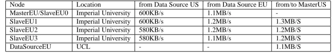
Table 2: PlanetLab EU inter-cluster and intra-cluster transmission speed
Node Location from Data Source US from Data Source EU from/to MasterUS MasterEU/SlaveEU0 Imperial University 600KB/s 1.1MB/s
-SlaveEU1 Imperial University 600KB/s 1.2MB/s 1.3MB/S SlaveEU2 Imperial University 580KB/s 1.2MB/s 1.2MB/S SlaveEU3 Imperial University 580KB/s 1.1MB/s 1.2MB/S
DataSourceEU UCL - - 1.1MB/S
Table 3: PlanetLab workload and data configurations
Workload Data source Aggregation Input Size
Wordcount Plain-text High 800MB (400MB x 2) Wordcount Random data Ballooning 250MB (125MB x 2) Sort Random data Zero 250MB (125MB x 2)
We set the number of Reduce tasks to 2 for each workload. In the case where we separate the job into two disjoint MapReduce jobs, we give each of the two clusters a single Reduce task.
We implemented the MapReduce architectures as described in Section 3.1 with the two disjoint clusters being the nodes from US and EU, respectively. The specific architectural resource alloca-tions are as follows:
• Local MapReduce (LMR): 4 compute nodes in the US are
used along with the US and EU data sources.
• Global MapReduce (GMR): 2 compute nodes from the US,
2 compute nodes from EU, and both US and EU data sources are used.
• Distributed MapReduce (DMR): 2 compute nodes from the
US, 2 compute nodes from EU, and both US and EU data sources are used.
4.2
Amazon EC2
In our Amazon EC2 environment we used m1.small nodes, each of which was allocated 1 EC2 32-bit compute unit, 1.7 GB of RAM and 160 GB instance storage. We used nodes from EC2 data centers located in the US and Europe. The data transmission speeds we experienced between these data centers are shown in Table 4. As in the PlanetLab setup, the number of reducers was fixed at 2 in LMR and 1 per cluster in DMR. Our workload configurations can be seen in Table 5. We used data input sizes between 1–3.2 GB. Our EC2 experiment architectures were limited to LMR and DMR1and are
allocated as follows:
• Local MapReduce (LMR): 6 compute nodes in the US data
center are used along with the US and EU data sources.
1
Due to an IP addressing bug between public and private address usage on EC2, we were unable to get GMR to run across multiple EC2 data center locations.
Table 4: EC2 inter-cluster and intra-cluster transmission speed
From/To US EU US 14.3MB/s 9.9MB/s EU 5.8MB/s 10.2MB/s
Table 5: Amazon EC2 workload and data configurations
Workload Data source Aggregation Input Size Wordcount Plain-text High 3.2GB (1.6GB x 2) Wordcount Random data Ballooning 1GB (500MB x 2) Sort Random data Zero 1GB (500MB x 2)
• Distributed MapReduce (DMR): 3 compute nodes from the
US data center, 3 compute nodes from the EU data center, and both US and EU data sources are used.
4.3
Measuring Job Completion Time
We enumerate the steps needed for the MapReduce job to be completed under the selected architectures:
• Local MapReduce (LMR): Job completion time is
mea-sured from the time taken to insert data from both data sources into HDFS located in the main cluster plus the MapReduce runtime in the main cluster.
• Global MapReduce (GMR): Job completion time is
mea-sured from global HDFS data insertion from both data sources time plus global MapReduce runtime.
• Distributed MapReduce (DMR): Job completion time is
taken from the max time of both individual MapReduce jobs (plus HDFS push times) in the respective clusters (both must finish before the results can be combined), plus the result-combination step to combine the sub-results into the final re-sult at a single data location.
5.
EVALUATION
5.1
PlanetLab
We ran 4 trials of each of the three main experiments over the three architectures on PlanetLab. We measured and plotted each component of the job completion times:
0 200 400 600 800 1000 1200 1400 Push US Push EU
Map Reduce Result Combine
Total
Time (in seconds)
LMR GMR DMR
(a) Wordcount on 800MB plain-text data
0 100 200 300 400 500 600 700 800 Push US Push EU
Map Reduce Result Combine
Total
Time (in seconds)
LMR GMR DMR
(b) Wordcount on 250MB random data
0 50 100 150 200 250 300 350 400 450 500 Push US Push EU
Map Reduce Result Combine
Total
Time (in seconds)
LMR GMR DMR
(c) Sort on 250MB random data
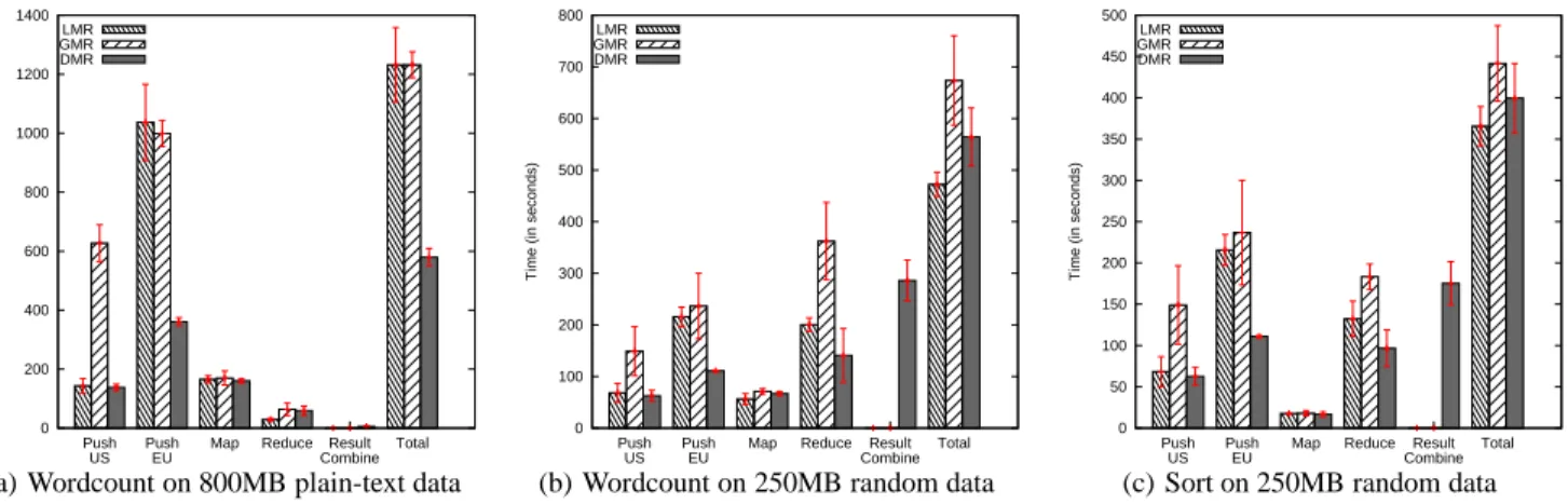
Figure 4: PlanetLab results. In the case of high-aggregation in (a), DMR finishes the fastest due to avoiding the transfer of input data over slow links. But in zero-aggregation and ballooning-data conditions, LMR finishes faster since it minimizes intermediate and output data transfer costs.
0 100 200 300 400 500 600 700 800 900 1000 Push US Push EU
Map Reduce Result Combine
Total
Time (in seconds)
LMR DMR
(a) Wordcount on 3.2GB of plain-text data
0 100 200 300 400 500 600 700 800 900 Push US Push EU
Map Reduce Result Combine
Total
Time (in seconds)
LMR DMR
(b) Wordcount on 1GB of random data
0 50 100 150 200 250 300 Push US Push EU
Map Reduce Result Combine
Total
Time (in seconds)
LMR DMR
(c) Sort on 1GB of random data
Figure 5: Amazon EC2 results. In the case of high aggregation in (a), DMR still outperforms LMR but at a smaller relative margin than PlanetLab due to higher inter-cluster bandwidth. LMR again outperforms DMR in zero-aggregation and ballooning-data scenarios where it is advantageous to centralize the input data immediately instead of waiting until the intermediate or output phases.
1. Push US is the time taken to insert the data from the US data source into the proper HDFS given the architecture,
2. Push EU, similar to Push US, is the time taken to insert the data from the EU data source into the proper HDFS,
3. Map is the Map-phase runtime,
4. Reduce is the residual Reduce-phase runtime after the Map progress has reached 100%,
5. Result-Combine is the combine phase for the DMR archi-tecture only, comprised of the data transmission plus combi-nation costs, assuming those could be done in parallel, and
6. Total is the total runtime of the entire MapReduce job.
We have plotted the averages as well as the 95th percentile confi-dence intervals.
High-Aggregation Experiment: We ran Wordcount on 800 MB
plain text. As seen in Figure 4(a), DMR completed 53% faster than the other architectural approaches. First of all, DMR benefits from parallelism by saving time from the initial HDFS data push trans-mission costs from both data sources. Since the data is only pushed
to its local HDFS cluster, and this is done in parallel in both clus-ters, we avoid a major bottleneck. LMR and GMR both transmit input data across clusters, which is costly in this environment.
Secondly, note that the Map and Reduce phase times are almost identical across the three architectures, since the Map tasks are run with local data, and the intermediate data is small due to the high aggregation factor.
Last, the result combine step for DMR is low since the output data is small. Therefore we see a statistically significant advantage in using the DMR architecture under our high-aggregation experi-ment.
Ballooning-data Experiment: We ran Wordcount on 250 MB
random binary data which resulted in an output size 1.8 times larger than the input size, since each “word” in the random data is unique and textual annotations to each word occurrence adds to the size of the output data.
As seen in Figure 4(b), DMR still benefits from faster HDFS push times from the data sources. However, since the intermediate and output data sizes are quite large, the result-combining step adds a large overhead to the total runtime. Even though the reduce phase appears to be much faster, this is because the final result-combining step is acting as a final reduce operation as well.
LMR is the statistically-significant best finisher in this experi-ment due to its avoidance of transmitting large intermediate and output data across the wide-area system (as in both GMR and DMR); instead, by just transmitting the input data across the two clusters, it comes out ahead, 16% and 30% faster than DMR and GMR, re-spectively.
Zero-Aggregation Experiment: We ran Sort on 250 MB
ran-dom binary data. As seen in Figure 4(c), this experiment has results similar to the ballooning-data experiment. However since there is less intermediate and output data than the previous experiment, the three architectures finish much closer to each other. LMR finishes only 9% faster than DMR and 17% faster than GMR.
Since there is zero aggregation occurring in this experiment, and it is merely shuffling the same amount of data around, only at dif-ferent steps, it makes sense that the results are very similar to each other. LMR transmits half the input data between clusters before the single MapReduce job begins; DMR transmits half the output data between the clusters after the half-size MapReduce jobs have been completed, only to encounter a similar-size result-combine step. DMR is also at a disadvantage if its workload partitioning is unequal, in which case one cluster would be waiting idle for the other to complete its half of the work.
GMR has a statistically worse performance than LMR primarily because some data blocks may travel between clusters twice (due to the location-unaware HDFS replication) instead of just once.
5.2
Amazon EC2
Our experiments in Amazon EC2 further confirmed our intu-itions behind our PlanetLab results, and provided even stronger statistically-significant results. We ran 4 trials of each of the three main experiments over the three architectures, plotting the averages and the 95th percentile confidence intervals.
High-aggregation Experiment: As seen in Figure 5(a), DMR
still outperforms LMR but by only 9%, a smaller relative margin than PlanetLab due to higher inter-cluster bandwidth. Also, be-cause of the high inter-cluster bandwidth, LMR incurs less of a penalty from transferring half the input data across data centers, which makes it a close contender to DMR.
Ballooning-data Experiment: As seen in Figure 5(b), LMR
outperforms DMR but at a slightly higher relative margin (44%) compared to our PlanetLab results (16%). LMR again avoids the cost of moving large intermediate and output data between clusters and instead saves on transfer costs by moving the input data before the job begins.
Zero-Aggregation Experiment: From Figure 5(c), our results
are quite similar to those from PlanetLab. LMR and DMR are al-most in a statistical tie, but DMR finishes in second place (by 21%) most likely due to the equal-partitioning problem where if one of the two clusters falls slightly behind in the computation, the other cluster finishes slightly early and then half the data center compute resources sit idle while waiting for the other half to finish. Instead with LMR, no compute resources would remain idle if there were straggling tasks.
5.3
Summary
In our evaluation we measured the performance of three separate MapReduce architectures over three benchmarks in two platforms, PlanetLab and Amazon EC2. In the case of a high-aggregation workload, we found that DMR significantly outperformed both LMR and GMR architectures since it avoids data transfer overheads of the input data.
However, in the case of zero-aggregation or ballooning-data sce-narios, LMR outperforms DMR and GMR since it moves the input
data to a centralized cluster, incurring an unavoidable data transfer cost at the beginning instead of at later stages, which allows the compute resources to operate more efficiently over local data.
6.
RECOMMENDATIONS
In this paper we analyzed the performance of MapReduce when operating over highly-distributed data. Our aim was to study the performance of MapReduce in three distinct architectures over vary-ing workloads. Our goal was to provide recommendations on which architecture should be used for different combinations of work-loads, data sources and network topologies.
We make the following recommendations from the lessons we have learned:
• For high-aggregation workloads, distributed computation
is preferred. This is true especially with high inter-cluster
transfer costs. In this case, avoiding the unnecessary transfer of input data around the wide-area system is a key perfor-mance optimization.
• For workloads with zero-aggregation or ballooning data,
centralizing the data (LMR) is preferred. This assumes
that an equal amount of compute resources could be allocated in an LMR architecture as a DMR or GMR setting.
• For distributed computation, equal partitioning of the
workload is crucial to the architecture being beneficial.
As seen with the sort benchmark on random data, DMR fell slightly behind LMR in both PlanetLab and EC2 results. Even a slightly unequal partitioning has noticeable effects, since compute resources sit idle while waiting for other sub-jobs to finish. If unsure about input partitioning, LMR or GMR should be preferred over DMR.
• If the data distribution and/or compute resource
distri-bution is asymmetric, GMR may be preferred. If we are
unable to decide where the local cluster should be located in consideration of LMR, and we are not able to equally-divide the computation in consideration of DMR where each sub-cluster should have a similar runtime over the disjoint data sets, then GMR is probably the most conservative decision.
• The Hadoop Namenode, by being made location-aware
or topology-aware, could make more efficient block repli-cation decisions. If we could insert data into HDFS such
that the storage locations are in close proximity to the data sources, this would in fact emulate DMR in a GMR-type architecture. The default block replication scheme assumes tightly-coupled nodes, either across racks (even with rack-awareness) in the same datacenter, or in a single cluster. In-stead, the goals change in a distributed environment where data transfer costs are much higher.
7.
RELATED WORK
Traditionally, the MapReduce [7] programming paradigm assumed the operating cluster was composed of tightly-coupled homoge-neous compute resources that are generally reliable. Previous work has shown that if this assumption is broken, that MapReduce/Hadoop performance suffers.
Work in [11] showed that in heterogeneous environments, the Hadoop performance greatly suffered from stragglers, simply from machines that were slower than others. When applying a new schedul-ing algorithm, these drawbacks were resolved. In our work, we
assume that nodes can be heterogeneous since they belong to dif-ferent data centers or locales. However, the loosely-coupled nature of the systems we address adds an additional bandwidth constraint problem, along with the problem of having widely-dispersed data sources.
Mantri [3] proposed strategies for detecting stragglers in duce in a pro-active fashion to improve performance of the MapRe-duce job. Such improvements are complementary to our techniques; our work is less concerned with node-level slowdowns and more fo-cused on high-level architectures for higher-level performance is-sues with resource allocation and data movement.
MOON [9] explored MapReduce performance in volatile, vol-unteer computing environments and extended Hadoop to provide improved performance under situations where slave nodes are un-reliable. In our work, we do not focus on solving reliability issues; instead we are concerned with performance issues of allocating compute resources to MapReduce clusters and relocating source data. Moreover, MOON does not consider WAN, which is a main concern in this paper.
Other work has focused on fine-tuning MapReduce parameters or offering scheduling optimizations to provide better performance. Sandholm et. al. [10] present a dynamic priorities system for im-proved MapReduce run-times in the context of multiple jobs. Our work is concerned with optimizing single jobs relative to data source and compute resource locations. Work by Shivnath [4] provided al-gorithms for automatically fine-tuning MapReduce parameters to optimize job performance. This is complimentary to our work, since these same strategies could be applied in our system after we determine the best MapReduce architecture, in each of our re-spective MapReduce clusters. MapReduce pipelining [6] has been used to modify the Hadoop workflow for improved responsiveness and performance. This would be a complimentary optimization to our techniques since they are concerned with the packaging and moving of intermediate data without storing it to disk in order to speed up computation time. This could be implemented on top of our architecture recommendations to improve performance.
Work in wide-area data transfer and dissemination includes GridFTP [8] and BitTorrent [5]. GridFTP is a protocol for high-performance data transfer over high-bandwidth wide-area networks. Such mid-dleware would further complement our work by reducing data trans-fer costs in our architectures and would further optimize MapRe-duce performance. BitTorrent is a peer-to-peer file sharing protocol for wide-area distributed systems. Both of these could act as mid-dleware services in our high-level architectures to make wide-area data more accessible to wide-area compute resources.
8.
CONCLUSION
In this paper, we have shown the traditional single-cluster MapRe-duce architecture may not suitable for situations when data and compute resources are widely distributed. We examined three ar-chitectural approaches to performing MapReduce jobs over highly distributed data and compute resources, and evaluated their per-formance over several workloads in two platforms, PlanetLab and Amazon EC2. As a result of the lessons learned from our experi-mental evaluations, we have provided recommendations for when to apply the various MapReduce architectures, as a function of sev-eral key parameters: workloads and aggregation levels, network topology and data transfer costs, and data partitioning. We learned that a local architecture (LMR) is preferred in zero-aggregation conditions, and distributed architectures (DMR) are preferred in high-aggregation and equal-partitioning conditions.
References
[1] Amazon EMR. http://aws.amazon.com/elasticmapreduce/. [2] Amazon EC2. http://aws.amazon.com/ec2.
[3] G. Ananthanarayanan, S. Kandula, A. Greenberg, I. Stoica, Y. Lu, and B. Saha. Reining in the outliers in map-reduce clusters. In Proceedings of OSDI, 2010.
[4] S. Babu. Towards automatic optimization of mapreduce pro-grams. In ACM SOCC, 2010.
[5] Bittorrent. http://www.bittorrent.com/.
[6] T. Condie, N. Conway, P. Alvaro, J. M. Hellerstein, K. Elmeleegy, and R. Sears. Mapreduce online. In
Proceed-ings of NSDI, 2010.
[7] J. Dean and S. Ghemawat. Mapreduce: Simplified data pro-cessing on large clusters. In Proc. of OSDI, 2004.
[8] Gridftp. http://globus.org/toolkit/docs/3.2/gridftp/.
[9] H. Lin, X. Ma, J. Archuleta, W.-c. Feng, M. Gardner, and Z. Zhang. Moon: Mapreduce on opportunistic environments. In Proceedings of the 19th ACM International Symposium on
High Performance Distributed Computing, HPDC ’10, 2010.
[10] T. Sandholm and K. Lai. Mapreduce optimization us-ing dynamic regulated prioritization. In ACM
SIGMET-RICS/Performance, 2009.
[11] M. Zaharia, A. Konwinski, A. D. Joseph, R. H. Katz, and I. Stoica. Improving mapreduce performance in heteroge-neous environments. In Proceedings of OSDI, 2008.