Wavelet transform‐based seismic facies classification and modelling: application to a geothermal target horizon in the NE German Basin

Wavelet transform-based seismic facies classification and modelling:

application to a geothermal target horizon in the NE German Basin

Klaus Bauer

_{, Ben Norden}

_{, Alexandra Ivanova}

_{, Manfred Stiller}

and Charlotte M. Krawczyk

1_{Deutsches GeoForschungsZentrum GFZ, Telegrafenberg, D-14473, Potsdam, Germany, and}2_{Technische Universit ¨at Berlin,} Ernst-Reuter-Platz 1, D-10587, Berlin, Germany

Received February 2019, revision accepted July 2019

A B S T R A C T

At the geothermal test site near Groß Sch ¨onebeck (NE German Basin), a new 3D seismic reflection survey was conducted to study geothermal target layers at around 4 km depth and 150°C. We present a workflow for seismic facies classification and modelling which is applied to a prospective sandstone horizon within the Rotliegend formation. Signal attributes are calculated along the horizon using the continuous Morlet wavelet transform. We use a short mother wavelet to allow for the temporal resolution of the relatively short reflection signals to be analysed. Time-frequency do-main data patterns form the input of a neural network clustering using self-organizing maps. Neural model patterns are adopted during iterative learning to simulate the in-formation inherent in the input data. After training we determine a gradient function across the self-organizing maps and apply an image processing technique called wa-tershed segmentation. The result is a pattern clustering based on similarities in wavelet transform characteristics. Three different types of wavelet transform patterns were found for the sandstone horizon. We apply seismic waveform modelling to improve the understanding of the classification results. The modelling tests indicate that thick-ness variations have a much stronger influence on the wavelet transform response of the sandstone horizon compared with reasonable variations of seismic attenuation. In our interpretation, the assumed thickness variations could be a result of variable paleo-topography during deposition of predominantly fluvial sediments. A distinct seismic facies distribution is interpreted as a system of thicker paleo-channels de-posited within a deepened landscape. The results provide constraints for the ongoing development of the geothermal test site.

Key words: Full waveform, Interpretation, Reservoir geophysics.

1 I N T R O D U C T I O N

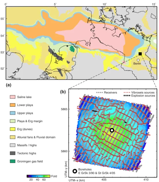
Geothermal energy is considered as one prospective compo-nent in a future mix of energy supply with reduced greenhouse gas emission. The research platform in Groß Sch ¨onebeck, lo-cated within the NE German Basin about 40 km north of Berlin (Fig. 1), was established to test exploration and

ex-∗_{E-mail: [email protected]}

ploitation technologies for the extraction of geothermal en-ergy from sedimentary and igneous target horizons of the Rotliegend formation at around 4 km depth and 150°C. A new 3D seismic survey was conducted in 2017 to deliver de-tailed knowledge on geological structures and reservoir char-acteristics, which is required for the improved understanding of observations made in the past and for the planning of en-visaged future drilling and stimulation activities (Krawczyk

0˚ 5˚ 10˚ 15˚ 52˚ 53˚ 54˚ 55˚ Berlin 5860 5865 405 410 20 40 60 Fold Vibroseis sources Explosion sources Receivers Boreholes E GrSk 3/90 & Gt GrSk 4/05 UTM−x (km) UTM−y (km) Saline lake Lower playa Upper playa Playa & Erg margin Erg (dunes)

Alluvial fans & Fluvial domain Massifs / highs

Tectonic highs Groningen gas field

(a)

(b)

Figure 1 Location map of the geothermal test site near Groß Sch ¨onebeck (NE German Basin). (a) Upper Rotliegend facies distribution in the Southern Permian Basin (after Gastet al.2010; Frybergeret al.2011; Henareset al.2014). (b) Location of vibroseis sources (red stars), explosion sources (black stars), receivers (grey circles) and resulting nominal fold distribution.

results from a seismic facies classification and modelling ap-plied to this new 3D seismic data. A sandstone horizon within the Rotliegend formation is used as an example to show the potential of our seismic facies interpretation approach for the characterization of geothermal reservoirs.

Seismic facies analysis is an efficient tool to study vari-ations of signal characteristics within sub-regions of seismic reflection data. Generally, variations in seismic facies are as-sumed to reflect geological facies variations to be mapped for reservoir characterization studies. The seismic facies is typically determined based on a series of signal attributes measuring properties such as amplitudes, frequency content

and their local distribution over time and space (e.g. Taner, Koehler and Sheriff 1979; Marfurtet al.1998; Chopra and Marfurt 2005; Barnes 2007). A large number of partly re-dundant signal attributes are available, which even can make choosing the useful parameters difficult in some cases (Barnes 2007). As an alternative to these more classical attributes, the Morlet wavelet transform delivers spectral amplitudes for the full range of measured frequencies (Grossman and Mor-let 1984). We consider the waveMor-let transform attributes as a kind of full waveform representative which can be used for a holistic characterization of the seismic reflection signals. The waveform-derived signal attributes are combined in different

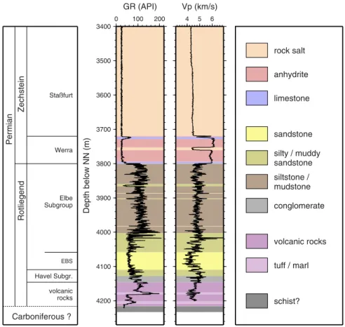
Permian Carboniferous ? Zechstein Rotliegend Staßfurt Werra Havel Subgr. Elbe Subgroup volcanic rocks EBS 3400 3500 3600 3700 3800 3900 4000 4100 4200 Depth below NN (m) 0 100 200 GR (API) 4 5 6 Vp (km/s) rock salt anhydrite limestone sandstone silty / muddy sandstone siltstone / mudstone conglomerate volcanic rocks tuff / marl schist? Figure 2 Litho-stratigraphy and

down-hole logging data (Gamma ray and sonic logs) at the E GrSk 3/90 well. The shown depth interval is focussing on the Rotliegend target horizon (EBS: Elbe base sandstone).

ways of multi-attribute analysis. Some approaches try to pre-dict reservoir properties based on correlations between seis-mic waveform signatures and physical properties determined in boreholes (e.g. Russellet al.1997; Trappe and Hellmich 2000; Hampson, Schuelke and Quirein 2001). The most com-mon way to combine multi-attribute information is cluster-ing analysis uscluster-ing statistical methods or neural network-based techniques (e.g. Col´eou, Poupon and Azbel 2003; de Matos, Osorio and Johann 2007; Pussaket al.2014; Molino-Minero-Reet al.2018). Facies types identified by the clustering analy-sis can be mapped to show their distribution across the geolog-ical targets. The interpretation is typgeolog-ically supported by rec-onciliation with available information from wells (e.g. Aleardi

et al.2015). In addition, the signal characteristics defining the seismic facies types may provide insight into their inherent geological nature (e.g. Pussaket al.2014). Ultimately, results from classification and mapping of seismic facies can be used to define geometric and petrophysical constraints for the con-struction of reservoir models.

Our workflow includes wavelet transform analysis of re-flection signals, classification of wavelet transform-based pat-terns using self-organizing maps and interpretation of

classi-fied patterns supported by seismic modelling. After a short introduction of the geological setting, experiment and data, we describe our method for the generation of data patterns. We also show details of our method of self-organizing maps, which include some modifications to facilitate the definition and visualization of clusters after the learning procedure. For the interpretation of the classification results, we apply seis-mic modelling based on borehole information. We chose this approach to improve the understanding of the found seismic facies characteristics as a contribution to overcome the kind of black box nature of neural network-based classification.

2 S T U D Y A R E A A N D D A T A

The study area is located in the NE German Basin (Fig. 1), which represents a sub-basin within the Southern Permian Basin (SPB). The entire SPB system extends from Middle England to North Germany, Poland and the Baltic States. The basin developed in response to thermal relaxation of Early Permian lithospheric thinning and related magmatic destabilization, crustal extension, tectonic subsidence and sedimentation (van Weeset al.2000). After a phase of Early

1.3 1.4 1.5 1.6 1.7 1.8 1.9 Time (s)

(a)

(b)

(c)

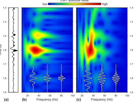
Figure 3(a) Seismic trace from the 3D seismic data. (b) Time-frequency spectrogram from continuous wavelet transform using a short mother wavelet withl =5/(2π). Exemplary wavelets are displayed for frequencies of 30, 55 and 80 Hz. (c) Time-frequency spectrum for a longer mother wavelet withl =10/(2π). Higher resolution in frequency is related with lower resolution in time and vice versa.

Permian volcanism, basin subsidence and sedimentation started in the Late Permian and lasted until Early Jurassic times. Generally, the North German Basin is considered, be-sides the northern foreland of the Alps and the Rhine graben, as a prospective region in Germany to make use of geothermal energy.

GFZ Potsdam is developing the geothermal test site in Groß Sch ¨onebeck as a research platform since 2000. The lo-cation had been selected as an exemplary site for geother-mal exploitation in the North German Basin based on criteria such as favourable temperature field, adequate porosity and permeability of potential target horizons, vicinity to poten-tial users (Berlin) and access to an existing borehole (Huenges and Hurter 2002). In the E GrSk 3/90 well at the geother-mal test site (Fig. 1), Carboniferous rocks are overlain by Rotliegend volcanics, conglomerates, sandstones, siltstones and mudstones (Fig. 2). The porous and permeable sand-stones and volcanic rocks of the Rotliegend are considered as potential target horizons for geothermal exploitation based on surrounding temperatures of 150°C. Here we focus on the sandstone formation, as the identification of the volcanic rocks in the seismic data appears less clear. The Rotliegend

sandstones formed under semi-arid to arid, sub-equatorial conditions. Topography and climatic conditions were major controlling factors of deposition (Gastet al.2010). Our study area (Fig. 1) is located within a transition zone characterized by eolian, fluvial and playa facies (Gastet al.2010; Fryberger

et al.2011). The major depocentre was located more towards the west (Saline lake in Fig. 1a) while sediment input was presumably delivered from the east where a minor swell sep-arates the NE German Basin from the Polish Trough. The targeted Rotliegend formation is overlain by carbonates, an-hydrite and halite of the Zechstein saliniferous successions (Fig. 2) widespread abundant in the SPB.

A first geological model was developed by use of borehole information and reinterpretation of sparse two-dimensional (2D) seismic reflection data from former industrial explo-ration within the region (Moeck, Schandelmeier and Holl 2009). A combined seismic tomography and magnetotelluric experiment within the European Union-funded I-GET project delivered a combined 2D model of seismic velocity and elec-trical resistivity (Baueret al.2010; Mu ˜nozet al.2010; Bauer, Mu ˜noz and Moeck 2012). A new well (Gt GrSk 4/05) was drilled and used in combination with the E GrSk 3/90 well

20 40 60 80 100 Frequency (Hz) 20 40 60 80 100 Frequency (Hz) −5 0 5 Time (ms) 20 40 60 80 100 Frequency (Hz) 1 2 3 4 5 6 7 8 n SOM nodes Input 1 2 3 n

(a)

(b)

(c)

Figure 4 (a) Exemplary subsection from processed 3D data. Continuous wavelet transform coefficients are determined within a short-time window centred at the picked reflection signal. (b) The time-frequency spectrograms are converted inton-dimensional data patterns. (c) The data patterns form the input for the self-organizing map (SOM).

for a series of hydraulic stimulation experiments to inves-tigate the feasibility of producing geothermal energy (e.g. Legarth, Huenges and Zimmermann 2005; Bl ¨ocher et al.

2016). These studies were accompanied by downhole mea-surements and core analysis for a petrophysical

characteriza-tion of the Rotliegend reservoir (e.g. Trautwein and Huenges 2005).

A new 3D seismic reflection experiment was conducted in 2017 (Stilleret al.2018; Krawczyket al.2019) in order to support further steps in the development of the geothermal

SOM component−1 (normalized) Iteration = 1 SOM component−2 (normalized) SOM component−n (normalized) Total gradient (normalized) Iteration = 200 Iteration = 500 Iteration = 25000 Iteration = 30000

Min Max Min Max

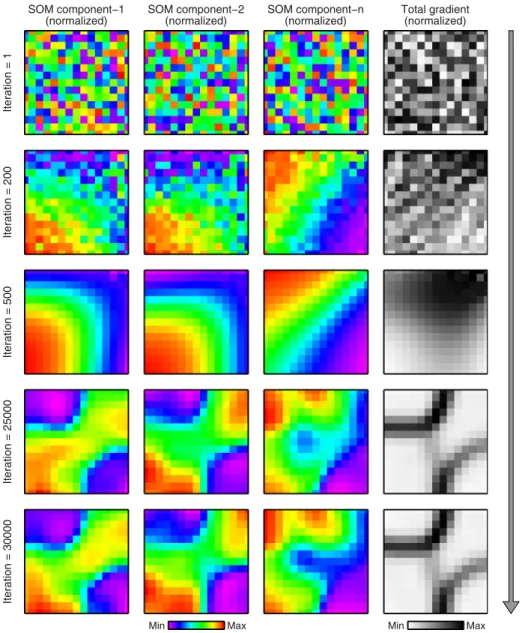
Figure 5 Development of the self-organizing map (SOM) during iterative learning. Rows correspond to different integration steps. Three left columns show examples of SOM components. The right column shows gradient function measured across the SOM. The grey arrow at the right side indicates progression of iterative learning.

research platform in Groß Sch ¨onebeck. The experimental lay-out was centred around the E GrSk 3/90 and Gt GrSk 4/05 wells and covered an area of about 8 by 8 km2 _{(Fig. 1b).}

Source and receiver points with spacings of 50 m were de-ployed along approximately EW running source lines and NS running receiver lines. Spacing between source and receiver lines was 700 m and 400 m, respectively. A total of 1830 vi-broseis points (4 vibrators, linear sweeps of 12–96 Hz) were complemented by 15 explosion shots (ca. 1.2 kg, 10–15 m depth). A total of 3240 receiver points with 10 Hz geophone groups were all active during the survey. A first processing of the data provided a post-stack time-migrated cube (Stiller

et al.2018; Krawczyket al.2019), which was further analysed by the methods described in this paper.

3 M E T H O D S

3.1 Continuous wavelet transform

Spectral decomposition methods are used to derive spec-tral amplitudes for given frequency bands or at discrete frequency values of interest. With such techniques, seismic reflection signals can be converted into sets of spectral attributes for the purpose of seismic facies classification.

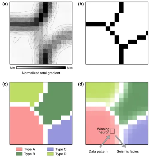
Figure 6(a) Gradient function after training. (b) A watershed segmentation algorithm is used to determine borders between regions of low gradient values. (c) Separated regions with low gradient values are assigned to colour-coded signal types based on underlying similarities in signal characteristics. (d) Colour saturation is weighted by the gradient function. Data patterns are finally classified as facies types based on the winning neuron with the most similar neural model pattern.

Examples of common spectral decomposition approaches include short-time Fourier transform, wavelet transform, S-transform and combinations of these approaches (e.g. Chakraborty and Okaya 1995; Castagna, Sun and Siegfried 2003; Sinhaet al.2005; Kazemeiniet al.2009; von Hartmann

et al.2012; Wu and Castagna 2017; Huanget al.2018). In our investigation, we used the continuous wavelet transform (CWT; e.g. Kumar and Foufoula-Georgiou 1997). This method has advantages against the windowed Fourier trans-form, particularly when spectral information is required with high resolution in both time and frequency as it is the case in the analysis of seismic reflection signals (e.g. Castagnaet al.

2003).

A time series signal f(t) is converted into the continuous wavelet transform of the signalW(s, τ) by use of the integral transform

W (s, τ)=

f(t)ψs,τ(t) dt. (1) In equation (1), the time series signalf(t) is multiplied by the wavelet functionψs,τ(t) which, in general form, is defined by ψs,τ (t)= 1 √ s ψ t−τ s . (2)

Equation (2) implies that a set of wavelet functionsψs,τ(t) is calculated from a so-called mother waveletψ(t) based on variations of the parameterss andτ. Scaling parameters is used to stretch and compress the wavelet. Parameterτ con-trols the location of the wavelet along the time axis. Different functions were introduced as mother wavelets, each suited for specific applications. When the sine-like Morlet wavelet (Grossmann and Morlet 1984) is used, the scaling parameter

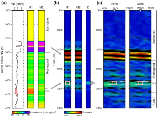
3500 3600 3700 3800 3900 4000 4100 4200 Depth below NN (m) 4 5 6 Vp (km/s) 10 12 14 16 Impedance (km/s*g/cm3₎ M1 M2 Zechstein Rotliegend EBS 1900 2000 2100 2200 2300 2400 Time (ms) M1 Envelope Min Max M2 D EBS 1900 2000 2100 2200 2300 2400 2360 2370 Inline 10390 10400 10410 Xline Zechstein Rotliegend EBS Carb.? (a) (b) (c)

Figure 7Identification of the EBS horizon based on modelling. (a) Models M1 with EBS and M2 without EBS are generated based on a smoothed sonic log from the E GrSk 3 well. (b) Synthetic seismograms from models M1 and M2. The difference of envelopes D reveals the location of the EBS in the time domain. (c) Assignment of the EBS horizon in the stacked and time-migrated data. Only a few traces inline and crossline around the well location (triangle) are shown.

s becomes a period (1/frequency) and equation (1) converts a one-dimensional (1D) time series into a two-dimensional (2D) time-frequency spectrum. A set of complex-valued Mor-let waveMor-lets with variable scalingsand shiftingτis determined by ψs,τ (t)= π−1/4_s−1/2_exp −i2πf0 t−τ s exp −1 2 t−τ s 2 . (3) Equation (3) represents an oscillating function weighted by a Gaussian envelope. Parameter f0 defines the basic

fre-quency of the mother wavelet, which relates to the number of oscillations below the Gaussian and, hence, to the length of the wavelet. Prokoph and Barthelmes (1996) introduced the parameterlto describe the length of the mother wavelet: ψl s,τ (t)= π−1/4_(sl)−1/2_exp −i2π1 s(t−τ) exp −1 2 t−τ sl 2 . (4) An example for the wavelet transform of seismic reflec-tion data is shown in Fig. 3. The 1D time series (Fig. 3a) is

converted into a 2D spectrum as a function of time and fre-quency (Fig. 3b,c). The 2D sampling in time and frefre-quency is obtained by variable values for parameterss andτ in equa-tions (1) and (4). A shorter and a longer mother wavelet (pa-rameterl in equation (4)) were used in the calculations to generate Fig. 3(b) and (c), respectively. The shorter mother wavelet withl =5/(2π) provides higher resolution in time (Fig. 3b), while the longer mother wavelet withl =10/(2π) provides higher resolution in frequency (Fig. 3c). This effect is related with the uncertainty principle, which said that res-olution cannot be arbitrarily small in both time domain and frequency domain (e.g. Prokoph and Barthelmes 1996). In the presented study, we used a relatively short mother wavelet withl =4/(2π) to emphasize temporal resolution because the analysed reflection signals are relatively short in time.

3.2 Self-organizing map

The self-organizing map (SOM; Kohonen 1982, 1990, 2001) is a neural network type, which is based upon competitive, unsupervised learning. One important field of application is pattern recognition and classification. In the case of seismic

5858 5860 5862 5864 5866 UTM−y (km) 402 404 406 408 410 UTM−x (km) E GrSk 3/90 Gt GrSk 4/05 S E N W

Type 1 Type 2 Type 3

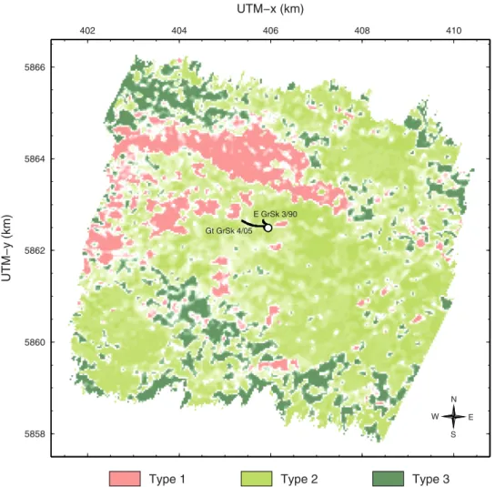
Figure 8 Results of wavelet transform-based signal classification for the EBS horizon. The analysed waveforms were clustered into three groups with specific signal characteristics. The distribution of seismic facies types is shown in a map view.

facies analysis, seismic signal characteristics are converted into data patterns, which serve as input information for the SOM. After learning, the input data patterns are clustered and the members of each cluster are classified as distinct seismic fa-cies types. Ultimately, the seismic fafa-cies types are interpreted as geological facies types. De Matoset al.(2007) suggested a workflow for seismic facies analysis including continuous wavelet transform and subsequent SOM clustering and clas-sification. In this study, we use a modified version of the ap-proach of de Matoset al.(2007) based on the SOM method of Baueret al.(2008, 2012, 2015).

The general workflow includes (a) preparation of data patterns, (b) unsupervised learning, (c) SOM segmentation and (d) classification of all data patterns. Figure 4 illustrates the preparation of data patterns. The seismic reflection hori-zon of interest is picked, and continuous wavelet transform coefficients are calculated for each trace using a given time

window centred at the picked time sample (Fig. 4a). Instead of using all data samples (e.g. de Matoset al.2007), we apply this data pre-selection step to exclude irrelevant signals and to restrict the information to the specified target horizon.

Data pattern vectors x are generated from the time-frequency domain CWT coefficientsw(s, τ) calculated at sin-gle traces within the short-time windows around the picked samples (Fig. 4a,b):

x=(w₁, w₂, w₃, . . . , w_n)T. (5)

The ordering and the meaning of indices for the CWT co-efficients are shown in Fig. 4(b). Noteworthy, the choice of the ordering is not critical because of a subsequent normalization procedure: For each component of the data pattern vectors, the mean and standard deviation for all data are determined and used in the normalization of each component (e.g. Bauer

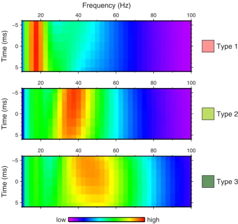
−5 0 5 Time (ms) 20 40 60 80 100 Frequency (Hz) Type 1 −5 0 5 Time (ms) 20 40 60 80 100 Type 2 −5 0 5 Time (ms) 20 40 60 80 100 Type 3 low high CWT absolute value

Figure 9 Results of wavelet transform-based signal classification for the EBS horizon. All data patterns which belong to the same seismic facies type are gath-ered and averaged.

inherent information of each data vector component is equally treated within the SOM analysis.

The data pattern vectorsx serve as input for the SOM (Fig. 4c). The SOM consists of a two-dimensional arrange-ment of neurons. Each neuron is associated with a model pattern vectormwith the same dimensionnas the data pat-tern vector. Hence, the SOM can be considered asnlayers, each representing one component of the model pattern vectors associated with the neurons (Fig. 4c). At the first step of the learning phase, the model vector components of all neurons are initialized by random values (upper row in Fig. 5). During each iterationtof the learning phase, a data pattern vectorxj is randomly chosen, and the so-called winning model pattern vectormwwith the smallest Euclidean distance (L2norm) to

the data pattern vector is determined:

∀i,||x(t)−m_w(t)||2<||x(t)−mi(t)||2. (6)

The model pattern vectors of all neuronsi are then up-dated by

mi(t+1)=mi(t)+λ(t)ηw,i(t) (x(t)−mi(t)), (7)

with learning rateλand neighbourhood functionη: ηw,i(t)=exp − r 2 w,i 2σ2_(t) , (8)

wherer_w,iis the distance between winning neuronwand neu-ron i at the SOM, and parameter σ controls the width of the Gaussian-weighting function. Equation (7) means that all model pattern vectors are modified in a way that they are more similar to the presented data pattern vectors after the opera-tion. This modification is strongest at the winning neuron and its neighbourhood because of the Gaussian-weighting func-tion (equafunc-tion (8)). With increasing iterafunc-tion numbers during the learning phase, the random distribution of model pattern vector components is changing into an ordered distribution across the SOM (see three left columns in Fig. 5). This self-organization process is an effect of equations (7) and (8). Learning continues until changes of the model pattern vectors are getting smaller than a given threshold value.

As a result of the learning phase, similar input data are associated with neighbouring neurons at the trained SOM. We use a total gradient functiongto identify regions at the

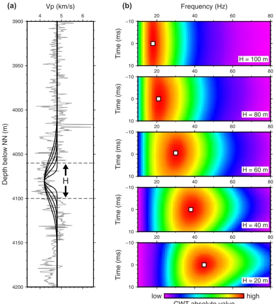
3900 3950 4000 4050 4100 4150 4200 Depth below NN (m) 4 5 6 Vp (km/s)

H

Figure 10 Seismic modelling of assumed thickness variations for the EBS horizon. (a) A simplified model description is based on measured sonic log velocities (grey line) in the E GrSk 3/90 well. The EBS horizon is described by a Gaussian-shaped velocity reduction. (b) Calculated time-frequency spectrograms for models with different thicknessH.

SOM, which have similar model pattern vectors and which are separated from other regions at the SOM by a strong gradient. The total gradient functiongifor neuroniis determined by

gi = 1 n n k=1 _∂m i,k ∂x 2 + _∂ mi,k ∂y 2 , (9)

wheren is the dimension of the model pattern vector with componentsm_i,k, andxandyrepresent the axes of the two-dimensional SOM, respectively. The development of the gra-dient function during the learning phase is illustrated in the right column of Fig. 5. The gradient function of the trained SOM (last iteration of the learning phase) is analysed by a

segmentation procedure to define clusters of model pattern vectors, which ultimately represent seismic facies types. A wa-tershed segmentation algorithm (Bauer et al. 2012) is used to identify the boundaries between regions with small gra-dients at the SOM (Fig. 6a,b). For each separated region, a distinct colour code is defined (Fig. 6c). Finally, the gra-dient function is used to define the colour saturation for each seismic facies type (Fig. 6d). In the application step, each data pattern vector is presented to the trained SOM and the corresponding winning neuron is determined by test-ing equation (6). The location of the winntest-ing neuron at the SOM defines the seismic facies type and related colour code (Fig. 6d).

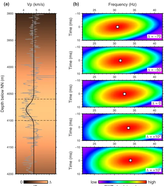
0 Δ dQp 3900 3950 4000 4050 4100 4150 4200 Depth below NN (m) 4 5 6 Vp (km/s)

(a)

(b)

Figure 11 Seismic modelling of assumed variable seismic attenuation (Q_p) for the EBS horizon. (a) A simplified model description is based on measured sonic log velocities (grey line) in the E GrSk 3/90 well. Seismic attenuation is modelled by perturbations ofQp(colour-coded) super-imposed on a reference model with constantQ_p=80. (b) Calculated time-frequency spectrograms for models with differentQ_pperturbations.

4 R E S U L T S A N D D I S C U S S I O N

The above-described workflow was applied for the analysis of the Rotliegend sandstone horizon. The Elbe base sandstone (EBS) is a well-pronounced porous sandstone at the bottom of the Elbe subgroup which is distributed in the marginal areas of the NE German Basin (Gastet al.1998; McCann 1998). In the E GrSk 3/90 well, the EBS is encountered between 4060 m and 4100 m depth where it shows low, only weakly varying Gamma ray values and decreased P-wave velocity in the sonic log (Fig. 2). The characteristic decrease in P-wave velocity is

caused by an increase of porosity (Trautwein and Huenges 2005).

To ensure which part of the waveforms in the processed data represents the EBS layer, we applied finite difference (FD) elastic forward modelling and compared synthetic data with the stacked and time-migrated data at the E GrSk 3/90 well. The modelling was based on a smoothed version of the P-wave velocity from the sonic log (Fig. 7a). Simplified assumptions were made on density (Gardner, Gardner and Gregory 1974) and onVsby using (Vp/Vs)2 _{= 3. The resulting impedance}

5858 5860 5862 5864 5866 UTM−y (km) 402 404 406 408 410 UTM−x (km) I−GET profile

f l u v i a l

p l a i n

Distance along I−GET profile (km)

−2 0 2

dVp (%)

S N

(a)

(b)

Figure 12 (a) Interpretation of seismic facies along the EBS horizon. Distribution of different seismic facies types is shown in a map view. Estimates on thickness and attenuation (Qp) are based on seismic modelling. Arrows show assumed direction of major sediment input. (b) Subsection of new 3D reflection data extracted along the I-GET profile.Pvelocity anomaly derived by travel time tomography and conversion to time domain (after Baueret al.2010). White line indicates target horizon, and red line coincides with low velocity anomaly interpreted as fault zone in Baueret al.(2010).

M2 where the velocity reduction between 4060 m and 4100 m depth associated with the EBS layer was eliminated (Fig. 7a). Synthetic data for the models M1 and M2 were calculated using the FD method of Bohlen (2002). The source wavelet used in these calculations was extracted from the measured data. The centre frequency of the extracted source wavelet was 52 Hz. The differences D of the envelopes between syn-thetics from M1 and M2 efficiently reveal the effect of the EBS (Fig. 7b) in the time domain data. We used this information to identify the targeted horizon in the stacked and time-migrated data (Fig. 7c).

The horizon was then picked within the entire data cube. We have picked the waveforms at the zero-crossing of the identified reflection signal in correspondence to the modelling results described above. A wavelet transform pattern was de-termined for each picked signal as illustrated in Fig. 4. One pattern consisted of CWT coefficients for frequencies between 10 and 100 Hz at 2.5 Hz intervals, calculated for each of seven time samples around the travel time pick. The time window was chosen to incorporate variations of the signal spectrum around the picked time. Tests with different time windows provided similar results, indicating a certain robustness re-garding this parameter. Altogether, 87,300 wavelet transform patterns were analysed using the self-organizing map (SOM) method of Baueret al.(2008, 2012, 2015). The CWT patterns were clustered into three different types of reflection signals. Figure 8 shows the distribution of these signal types across the Rotliegend EBS horizon.

An important question at this point is, if the results of the signal classification and mapping could be partly influenced by irregularities in the survey geometry, distribution of different source types and parameters used in the processing scheme. Comparison of Figs 1(b) and 8 shows no undesired correlation between the nominal fold and the distribution of signal types along the target horizon. Spectral analysis of signals measured near to the vibroseis and explosion source locations did not show significant and systematic differences in the frequency content. Tests with different processing parameters and dif-ferent stacking techniques did not show undesired changes in the wavelet transform output and SOM analysis results.

To understand the geological meaning of the different signal types, it is essential to evaluate their defining charac-teristics. For this purpose, we gathered all individual patterns which belong to the same signal type and determined their representative by arithmetic averaging of each CWT compo-nent (Fig. 9). Following this characterization, Type 1 (red colour) shows largest amplitudes around 17–20 Hz, Type 2 (light green colour) around 30–45 Hz and Type 3 (dark green

colour) around 35–60 Hz. In general, variations in reflec-tion signal characteristics or seismic facies can be related with a series of lithological properties, including layer thickness, composition of the rock matrix, porosity and pore filling, di-agenetic variations, amongst others. In our interpretation, we concentrate on two factors which are known for a strong influence on the frequency content of the reflection signal: thickness variations and variations of seismic attenuation (Figs 10 and 11).

We used FD viscoelastic modelling (Bohlen 2002) based on downhole logging data from the E GrSk 3/90 well to inves-tigate the potential effects of variable thickness and seismic at-tenuation on the wavelet transform pattern of the Rotliegend EBS reflection signal. For the modelling of thickness varia-tions, we generated a simplified model description with a con-stant P-wave velocity of 4.8 km/s and a velocity reduction of 0.6 km/s for the EBS. As the measured sonic log shows a more gradual transition instead of a sharp change at the top and bottom of the layer, we used a Gaussian function to describe the low velocity anomaly (Fig. 10a). Because of incomplete density logging data, density was calculated from P-wave velocity (method of Gardneret al.1974). Seismic at-tenuation (Q_p) was fixed with an assumed constant value of 80 based on laboratory data for sandstones (Toks ¨oz, John-ston and Timur 1979). Attenuation of S-waves (Q_s) was set equal toQ_p in all calculations. Synthetic traces were calcu-lated for models with different thickness (20 m, . . . , 100 m) of the low velocity layer, and CWT patterns were determined from the reflection signal. The results show a strong depen-dency of the frequency content on thickness (Fig. 10b). Based on this simplified modelling, we can explain the observed CWT patterns (Fig. 9) by predominant thickness of 80–100 m for Type 1 (red colour), around 40 m for Type 2 (light green colour) and around 20 m for Type 3 (dark green colour). In fact, these results are in agreement with a thickness of 39 m at the E GrSk 3/90 well, which is located within facies Type 2, and 22 m at the E GrSk 2/76 well, which is located within facies Type 3 (Fig. 12).

The potential influence of seismic attenuation on the CWT response was based on a model with a 40 m thick zone of reduced P-wave velocity and a variable Qp perturba-tion around the target layer (Fig. 11a). The modelling results indicate, that a decrease in Qp (increased attenuation) will produce large CWT amplitudes at slightly lower frequencies (Fig. 11b). An increase of Qp (decreased attenuation) leads to a shift of high CWT amplitudes towards slightly higher frequencies. In general, the simplified modelling tests indicate that thickness variations have a much larger influence on the

CWT response of the EBS layer compared with reasonable variations of Qp.

Our final interpretation of the seismic facies distribu-tion along the Rotliegend EBS horizon is based on the presented modelling results, borehole information and pre-existing knowledge on the geological facies from integration of regional data (e.g. Gastet al.1998; Gastet al.2010; Fry-bergeret al. 2011). Based on this information, we assume a predominantly fluvial facies in the studied area. The red-coloured facies (Type 1) is interpreted as a system of paleo-channels (Fig. 12). These parts are related with larger thickness of 80–100 m. If we assume an increase in seismic attenuation (decrease inQp), the thickness could be smaller than 80–100 m but still significantly larger than that for the other facies types. The paleo-channels with greater thickness could have been formed within a broader fault zone potentially affected by erosion at the paleo-surface, which would offer a larger space for deposition of sediments. This idea is supported by results of Baueret al.(2010), where a fault zone was inter-preted along those parts of a 2D tomographic model which are crossing the paleo-channels (dashed segment at I-GET pro-file in Fig. 12). We assume that the paleo-channels developed within a fluvial plain, which shows a predominant thickness of 40 m (Type 2, light green colours in Fig. 12). The fluvial sedimentation was most likely fed from the east, where a to-pographic swell existed between the NE German Basin and the Polish Trough (e.g. Gastet al.2010). Thinner sediments (Type 3, dark green colour in Fig. 12) could be partly related with topographic highs and less space for deposition of sed-iments. Such paleo-topographic highs may have existed as a result of the underlying structure (e.g. Baltrusch and Klarner 1993).

5 C O N C L U S I O N S

We used the continuous wavelet transform as a full waveform attribute description of reflection signals from a Rotliegend sandstone horizon and evaluated the results in context with geothermal exploration. Self-organizing map (SOM) classi-fication delivered three different seismic facies types which are mapped across the reflector. An important step in our interpretation is the visualization of the underlying average CWT patterns. Characteristic differences were found in the frequency content of each facies type. We used finite differ-ence modelling based on borehole information to investigate the potential influence of variable thickness and seismic at-tenuation on the CWT response of the analysed horizon. We consider the presented modelling approach as an example for

a possible interpretation strategy to improve understanding of seismic facies classification results.

The modelling results show that the observed seismic fa-cies variations can be mainly explained by thickness variations of the sandstone layer. We speculate that thickness variations were controlled by paleo-topographic variations and related variable accumulation space for predominantly fluvial sedi-ments. Thicker paleo-channels were found within a fault zone north of the E GrSk 3/90 and Gt GrSk 4/05 wells. Also, the un-derlying structure may have influenced paleo-topography and deposition of the sandstones. The results provide constraints for the continuing site development, including the planning of future drilling and geothermal production tests. The lat-eral distribution of the seismic facies types and their thickness variations can be used to describe the geometry of the sand-stone horizon within a new reservoir model. The required assignment of material properties within such a model will be based on our interpretation of paleo-channels. Assumed vari-ations in seismic attenuation together with petrophysical data could further support the definition of material properties. We propose an updated reservoir modelling for Groß Sch ¨onebeck based on the new 3D seismic data to investigate the behaviour of the geothermal reservoir during future production activi-ties.

Generally, the presented workflow could be extended if more wells would be available within the seismic study area. In such cases, direct estimation of thickness variations from spectral decomposition and SOM analysis would be possible (Yeet al.2019).

A C K N O W L E D G E M E N T S

The seismic experiment was financed by the Federal Ministry for Economic Affairs and Energy (BMWi grant 0324065). The authors would like to thank the contractor companies and all people involved in the fieldwork. Support by responsible authorities and local communities is gratefully acknowledged. Ariane Siebert helped to prepare figures. We thank two anony-mous reviewers and the Associate Editor for helpful comments and suggestions.

O R C I D

Klaus Bauer https://orcid.org/0000-0002-7777-2653

Ben Norden https://orcid.org/0000-0003-2228-9979

Charlotte M. Krawczyk

R E F E R E N C E S

Aleardi M., Mazzotti A., Tognarelli A., Ciuffi S. and Casini M. 2015. Seismic and well log characterization of fractures for geothermal exploration in hard rocks.Geophysical Journal International203, 270–283.

Baltrusch S. and Klarner S. 1993. Rotliegend-Gr ¨aben in NE Bran-denburg.Zeitschrift der Deutschen Geologischen Gesellschaft144, 173–186.

Barnes A.E. 2007. Redundant and useless seismic attributes. Geo-physics72, P33–P38.

Bauer K., Kulenkampff J., Henninges J. and Spangenberg E. 2015. Lithological control on gas hydrate saturation as revealed by sig-nal classification of NMR logging data.Journal of Geophysical Research Solid Earth120, 6001–6017.

Bauer K., Moeck I., Norden B., Schulze A., Weber M. and Wirth H. 2010. Tomographic P-wave velocity and vertical gradient structure across the geothermal site Groß Sch ¨onebeck (NE German Basin): relationship to lithology, salt tectonics, and thermal regime.Journal of Geophysical Research115, B08312.

Bauer K., Mu ˜noz G. and Moeck I. 2012. Pattern recognition and lithological interpretation of collocated seismic and magnetotel-luric models using self-organizing maps.Geophysical Journal In-ternational189, 984–998.

Bauer K., Pratt R.G., Haberland C. and Weber M. 2008. Neural network analysis of crosshole tomographic images: the seismic sig-nature of gas hydrate bearing sediments in the Mackenzie Delta (NW Canada).Geophysical Research Letters35, L19306. Bl ¨ocher G., Reinsch T., Henninges J., Milsch H., Regenspurg S.,

Kummerow J.et al.2016. Hydraulic history and current state of the deep geothermal reservoir Groß Sch ¨onebeck.Geothermics63, 27–43.

Bohlen T. 2002. Parallel 3-D viscoelastic finite difference seismic mod-elling.Computers and Geosciences28, 887–899.

Castagna J.P., Sun S. and Siegfried R.W. 2003. Instantaneous spec-tral analysis: detection of low-frequency shadows associated with hydrocarbons.The Leading Edge22, 120–127.

Chakraborty A. and Okaya D. 1995. Frequency time decomposition of seismic data using wavelet based methods.Geophysics60, 1906– 1916.

Chopra S. and Marfurt K.J. 2005. Seismic attributes – a historical perspective.Geophysics70, 3SO–28SO.

Col´eou T., Poupon M. and Azbel K. 2003. Unsupervised seismic facies classification: a review and comparison of techniques and implementation.Leading Edge22, 942–953.

de Matos M.C., Osorio P.L.M. and Johann P.R.S. 2007. Unsupervised seismic facies analysis using wavelet transform and self-organizing maps.Geophysics72, P9-P21.

Fryberger S.G., Knight R., Hern C., Moscariello A. and Kabel S. 2011. Rotliegend facies, sedimentary provinces, and stratigraphy, Southern Permian Basin UK and The Netherlands: a review with new observations. In: The Rotliegend of the Netherlands, vol. 98 (eds J. Gr ¨otsch and R. Gaupp), pp. 51–88. SEPM, Special Publications.

Gardner G.H.F., Gardner L.W. and Gregory A.R. 1974. Formation velocity and density – the diagnostic basics for stratigraphic traps. Geophysics39, 770–780.

Gast R.E., Dusar M., Breitkreuz C., Gaupp R., Schneider J.W., Stem-merik L.et al.2010. Rotliegend. In:Petroleum Geological Atlas of the Southern Permian Basin Area(eds J.C. Doornenbal and A.G. Stevenson), pp. 101–121. Houten, The Netherlands:EAGE Publi-cations b.v.

Gast R., Pasternak G., Piske J. and Rasch H.J. 1998. Das rotliegend im nordostdeutschen raum: Regionale ¨Ubersicht, Stratigraphie, Fazies und Diagenese.Geologisches Jahrbuch A149, 59–79.

Grossmann A. and Morlet J. 1984. Decomposition of Hardy functions into square integrable wavelets of constant shape.SIAM Journal on Mathematical Analysis15, 723–736.

Hampson D.P., Schuelke J.S. and Quirein J.A. 2001. Use of multi-attribute transforms to predict log properties from seismic data. Geophysics66, 220–236.

Henares S., Bloemsma M.R., Donselaar M.E., Mijnlieff H.F., Red-josentono A.E., Veldkamp H.G.et al.2014. The role of detrital an-hydrite in diagenesis of aeolian sandstones (Upper Rotliegend, The Netherlands): implications for reservoir-quality prediction. Sedi-mentary Geology314, 60–74.

Huang Y., Zheng X., Duan Y. and Luan Y. 2018. Robust time-frequency analysis of seismic data using general linear chirplet transform.Geophysics83, V197–V214.

Huenges E. and Hurter S. 2002. In-situ Geothermielabor Groß Sch ¨onebeck 2000/2001: Bohrarbeiten, Bohrlochmessungen, Hy-draulik, Formationsfluide, Tonminerale.Scientific Technical Re-port STR 2/14, Geothermie Report 02-1, GFZ Potsdam, 190 p.

Kazemeini S.H., Juhlin C., Zinck-Jørgensen K. and Norden B. 2009. Application of the continuous wavelet transform on seis-mic data for mapping of channel deposits and gas detection at the CO2Sink site, Ketzin, Germany.Geophysical Prospecting57, 111– 123.

Kohonen T. 1982. Self-organized formation of topologically correct feature maps.Biological Cybernetics43, 59–69.

Kohonen T. 1990. The self-organizing map.Proceedings of the IEEE 78, 1464–1480.

Kohonen T. 2001.Self-Organizing Maps, 3rd edn. Vol.30. Springer Series in Information Sciences. Berlin, Heidelberg: Springer. Krawczyk C.M., Stiller M., Bauer K., Norden B., Henninges J.,

Ivanova A. et al. 2019. 3-D seismic exploration across the deep geothermal research platform Groß Sch ¨onebeck north of Berlin/Germany.Geothermal Energy7, 1–18.

Kumar P. and Foufoula-Georgiou E. 1997. Wavelet analysis for geo-physical applications.Reviews of Geophysics35, 385–412. Legarth B.A., Huenges E. and Zimmermann G. 2005. Hydraulic

frac-turing in a sedimentary geothermal reservoir: results and implica-tions.International Journal of Rock Mechanics and Mining Sci-ences42, 1028–1041.

Marfurt K.J., Kirlin R.L., Farmer S.C. and Bahorich M.S. 1998. 3-D seismic attributes using a semblance-based coherency algo-rithm.Geophysics63, 1150–1165.

McCann T. 1998. The Rotliegend of the NE German Basin: back-ground and prospectivity.Petroleum Geoscience4, 17–27. Moeck I., Schandelmeier H. and Holl H.G. 2009. The stress regime

in a Rotliegend reservoir in the Northeast German Basin. Interna-tional Journal of Earth Sciences98, 1643–1654.

Molino-Minero-Re E., Rubio-Acosta E., Ben´ıtez-P´erez H., Brandi-Purata J.M., P´erez-Quezadas N.I. and Garc´ıa-Nocetti D.F. 2018. A method for classifying pre-stack seismic data based on amplitude-frequency attributes and self-organizing maps. Geophys-ical Prospecting66, 673–687.

Mu ˜noz G., Bauer K., Moeck I., Schulze A. and Ritter O. 2010. Ex-ploring the Groß Sch ¨onebeck (Germany) geothermal site using a statistical joint interpretation of magnetotelluric and seismic to-mography models.Geothermics39, 35–45.

Prokoph A. and Barthelmes F. 1996. Detection of nonstation-arities in geological time series: wavelet transform of chaotic and cyclic sequences. Computers and Geosciences 22, 1097– 1108.

Pussak M., Bauer K., Stiller M. and Bujakowski W. 2014. Improved 3D seismic attribute mapping by CRS stacking instead of NMO stacking: application to a geothermal reservoir in the Polish Basin. Journal of Applied Geophysics103, 186–198.

Russell B., Hampson D., Schuelke J. and Quirein J. 1997. Multiat-tribute seismic analysis.The Leading Edge16, 1439.

Sinha S., Routh P.S., Anno P.D. and Castagna J.P. 2005. Spectral decomposition of seismic data with continuous-wavelet transform. Geophysics70, P19–P25.

Stiller M., Krawczyk C.M., Bauer K., Henninges J., Norden B., Huenges E.et al.2018. 3D-Seismik am Geothermiestandort Groß Sch ¨onebeck.bbr – Fachmagazin f ¨ur Brunnen- und Leitungsbau 1/2018, 84–91.

Taner M.T., Koehler F. and Sheriff R.E. 1979. Complex seismic trace analysis.Geophysics44, 1041–1063.

Toks ¨oz M.N., Johnston D.H. and Timur A. 1979. Attenuation of seis-mic waves in dry and saturated rocks: i. Laboratory measurements. Geophysics44, 681–690.

Trappe H. and Hellmich C. 2000. Using neural networks to pre-dict porosity thickness from 3D seismic data.First Break18, 377– 384.

Trautwein U. and Huenges E. 2005. Poroelastic behaviour of phys-ical properties in Rotliegend sandstones under uniaxial strain. In-ternational Journal of Rock Mechanics and Mining Sciences42, 924–932.

van Wees J.D., Stephenson R.A., Ziegler P.A., Bayer U., McCann T., Dadlez R.et al.2000. On the origin of the Southern Permian Basin, Central Europe.Marine and Petroleum Geology 17, 43– 59.

von Hartmann H., Buness H., Krawczyk C.M. and Schulz R. 2012. 3-D seismic analysis of a carbonate platform in the Molasse Basin – reef distribution and internal separation with seismic attributes. Tectonophysics572–573, 16–25.

Wu L. and Castagna J. 2017. S-transform and Fourier transform frequency spectra of broadband seismic signals.Geophysics82, O71–O81.

Ye Y., Zhang B., Niu C., Qi J. and Zhou H. 2019. The thickness imaging of channels using multiple-frequency components analysis. Interpretation7, B1–B8.