Integration of System Dependability and Software
Reliability Growth Models for E-Commerce Systems
Myron Hecht, Yutao He, Herbert Hecht, and Xuegao An SoHaR Incorporated
8421 Wilshire Blvd. Suite 201 Beverly Hills, CA 90211
{myron, yutao, herb, xuegao}@sohar.com
Abstract
This paper describes how MEADEP [SoHaR00], a system level dependability prediction tool, and SMERFS [Farr93], a software reliability growth prediction tool can be used together to predict system reliability, and availability growth) for complex systems. The Littlewood/Verrall model is used to predict reliability growth from software test data. This prediction is integrated into a system level Markov model that incorporates WAN (Internet) service interruptions, hardware failures and recoveries, redundancy, coverage failures, and capacity. The results of the combined model can be used to predict the contribution of additional testing upon availability, the economic value of additional testing, and a variety of other figures of merit that support management decisions.
1.
Introduction
Growing expectations of immediate and dependable access to information is driving the need for higher fidelity measurement, modeling, and prediction – particularly in high transaction rate e-commerce applications. In such systems, availability has become the single most important attribute. In the words of the Chief Information Officer (CIO) of one of the 10 largest traffic web sites, “Availability is as important as breathing in and out [is] to human beings” [Fisher00]. Major web site and on-line information system outages now regularly make the front pages of major general circulation newspapers, and availability affects the market valuation of all firms doing significant amounts of commerce over the Internet.
E-commerce systems are complex on-line interactive systems incorporating custom developed applications with commercial off the shelf (COTS) hardware, COTS software, Internet gateways, and multiple Internet
service providers. Due to a variety of causes, applications developed for large Internet sites are constantly being modified and enhanced. However, there is significant pressure to minimize the development and test schedule for such software and as a result, it is not always mature when placed into service. Although COTS components are generally more mature and change much less rapidly than the custom developed applications, in large systems with many such components, failures occur frequently. Thus, both developed applications and COTS contribute to system undependability. The results of a recent survey of 40 managers of e-Commerce systems showed that application software was the leading cause of site degradations, but that WAN service provider and server hardware failures were the leading causes of unscheduled total site outages [Metz00].
Traditionally, there have been two separate disciplines of computer reliability modeling: (a) systems reliability, characterized by tools such as CARE III [Bavuso85], HARP [Trivedi85], SAVE [Goyal87], SHARPE [Sahner96], or UltraSAN [Sanders95] and (b) software reliability characterized by models such as the Schneidewind model, the generalized exponential model, the Musa/Okumoto Logarithmic Poisson model, and the Littlewood/Verrall model [ANSI92].
System reliability models use stochastic analysis and combinatorial probabilistic techniques to predict reliability. The underlying assumption in these measurement-based approaches is that the fundamental failure mechanisms are triggered stochastically, i.e., are non-deterministic (“Heisenbugs”). The most common modeling techniques are Markov chains and reliability block diagrams. Such models have been used to evaluate operational software based on failure data collected from commercial computer operating systems for more than a decade [Hsueh87, Tang92, Lee93]. System reliability/availability modeling has been used to
evaluate availability for air traffic control software systems [Tang95, Tang99, Rosin99]. The models account for non-deterministic hardware and software failures [Lee93, Tang95]. The limitations of system reliability models is that they assume constant failure and recovery rates. While assumption may be largely true for the hardware and the system software, which is usually stable, it is less true in the applications, which are constantly changing.
Software reliability growth models use measured time between error reports or number of error reports in a time interval. In most cases, they evaluate the reduction in failure frequency during successive developmental test intervals to estimate the software reliability at the end of a time period. The primary limitation of such models is that they do not account for system architectures, i.e., they assume software executed in a single processing processor or node [Schneidewind96]. They can not address systems that incorporate LANs, redundancy, and Wide Area Networks (WANs), all of which contribute to system downtime.
Thus, neither the software reliability nor system reliability approaches used independently are sufficient to model a current information system. Only an integrated software/system reliability model can accurately model the growing number of Internet-based systems being used for critical services such as medical information, financial transactions, e-Commerce, and Voice-over-IP. Integrated modeling and prediction methods can trade off such seemingly heterogeneous entities as the software testing program budget against the Service Level Agreements (SLAs) of an Internet Service Provider. An integrated model can address such questions as
• Given a known cost of downtime and current test
data, what is the economically optimal point at which to stop testing? What uptime benefit will be achieved by additional testing beyond this point?
• Based on current testing results, what is the highest
system availability that is likely to be achieved?
• How much more testing will be necessary in order
for the system to achieve the required availability?
• Is testing or additional redundancy a better strategy
for achieving availability goals?
Although there has been general recognition of the need to incorporate software and system reliability into a single model (see, for example, [LaPrie96] and
Wattanapongsakorn00]), there has been little work in integrated software reliability growth and system reliability modeling. In one of the few examples of previous work, Schneidewind [Schneidewind96] used a reliability block diagram approach to represent a client-server system in which he incorporated reliability growth models. In this paper, we extend this approach to a more complex hierarchical model consisting of both reliability block diagrams and Markov chains for a correspondingly larger system. We will then demonstrate how the impact of test time against capacity and availability can be assessed. Finally, we will demonstrate that substantive economic decisions on test strategies and stopping criteria can be developed using such a model.
2.
Methodology
The methodology for creating an integrated model consists of
1. Generating a system model that includes failure
rates and recovery times parameters for all significant system elements.
2. Substituting the appropriate reliability growth
equation for those parameters associated with software (primarily application software) whose reliability is changing (hopefully growing) in the course of the development period.
3. Evaluating the model and performing parametric
analyses to determine the impacts of various combination of parameters -- including
development time -- on overall system availability. We used two software tools to implement this methodology: MEADEP [SoHaR00] and SMERFS [Farr93].
MEADEP (Measurement-based Dependability) is a system-oriented reliability and availability measurement, modeling, and prediction tool with integrated data analysis modules. MEADEP uses analytical methods to evaluate block diagrams and Markov models. The models are created with a graphical user interface. The models can be hierarchical, allowing the analysis of large systems through decomposition. A key characteristic of MEADEP, its parser, enables the incorporation of failure rates, which, while constant during the evaluation of a particular model under the assumption of an exponential distribution, can be varied over the development cycle. The ability to incorporate a changing failure rate of this
type is the key to integrating the reliability growth predictions of SMERFS.
The software reliability prediction tool is SMERFS (Statistical Modeling and Estimation of Reliability Functions for Software) [Farr93], a well-known and widely accepted software application for evaluation of test data for failure rate and defect discovery rate prediction. The version of SMERFS used in this study included a total of 15 different reliability growth models. The input to SMERFS is a set of values consisting either of the time between discoveries of defects or the number of defects discovered per time period. SMERFS then uses maximum likelihood methods or least squares methods to estimate the parameters used for one or more of these models (depending on the type of input and user selected options). Its outputincludes the parameter estimates, predicted values and a measure of the goodness-of-fit using the chi-squared distribution [Farr88].
3.
Example of Integrated Model
To demonstrate the principle of the combined model, we will use the example of an e-commerce systems. In our example, we assume a 2-tiered architecture in which the first tier performs web page serving and handles other aspects of the user interface while the second performs database operations. This section discusses an analysis of the first tier, which consists of 11 COTS PC Servers running the Microsoft Windows NT 4 operating system, web server software, and an application for processing user input. The hardware, operating system, and web server software are COTS applications with a fixed failure rate that can be measured from the system log as described in [Hecht97]. However, the application software is under development, and software reliability growth predictions models are more appropriate.
Data for this example were selected from Data Set 1 in the SMERFS distribution included in [Farr96]. The data were fit to multiple software reliability models in the SMERFS program. The best fit model based on the results were the Littlewood/Verall Bayesian model [Littlewood80, ANSI92]. The linear form of failure rate is [Farr96] ) 1 ( 2 1 1 2+ − − = α β β α λ test o t Equation 1
in which the values of the α, βo, and β1 parameters were
determined by SMERFS.
Integration of this predicted failure rate with other COTS components of each server is represented by the Markov diagram shown in Figure 1. There are three states in the model: normal, PCSW_failed (any of the 3 major components of the server has suffered a failure
resulting in the loss of service), and PCHW_failed
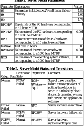
(server hardware failure). The numbers below the state name represent rewards, i.e., the value of the state. A reward of 1 means that the system is fully functional, a reward of 0 means that the system is completely failed. MEADEP allows intermediate values of reward (i.e., between 0 and 1) in order to represent partial loss of capability. The use of such partial rewards will be discussed below. Table 1 describes the parameters, and Table 2 describes the transitions.
The following points should be noted:
(a) There are 4 failure modes considered in the model:
hardware failure, application software failure, Internet server software failure, and operating system failure.
(b) The hardware failure is separated from software
failures because the hardware failure requires replacement (assumed to take 1 hour) vs. a software restoration that can be achieved by means of a restart (assumed to require 15 minutes), and
(c) The application software failure modes are assumed
to be crash, hang, and stop. We have not considered the case of an incorrect response with normal behavior because it is assumed that this type of error should have been removed during earlier development. Because the system being modeled is an e-Commerce application with relatively simple logic this is not an unreasonable assumption. However, by the addition of a state, incorrect response could be incorporated into the system model. For this failure mode, it would be more appropriate to use a model that predicts number of faults found rather than reliability (see for example, [Farr96]).
Figure 1 represents the Markov chain diagram for a single server, but as noted above, there are 11 front-end servers in the web site. The reliability growth model shown in Equation 1 is incorporated into the arc for software failures. Explanations of the variables, states and transitions are contained in Tables 1 and 2. Figure 2 shows how the model in Figure 1 is incorporated into a
higher level model that evaluates both the effects of redundancy and capacity loss.
Table 1. Server Model Parameters
Parameter Explanation Value
β1 1.86
α 1.06
β0
Parameters in Littlewood/Verall linear failure intensity
1.73
µPCHW Repair rate of the PC hardware, corresponding to a 1 hour MTTR
1
λPCHW Failure rate of the PC hardware, corresponding to a 1000 hour MTBF
0.001
µPC Restoration/restart rate of the PC hardware, corresponding to a 15 minute restart time
4
testtime Test time in hours 500
λWebserv Failure rate of the web server software, corresponding to a 1000 hour MTBF
0.001
λOS Failure rate of the operating system software, corresponding to a 1000 hour MTBF
0.001
Table 2. Server Model States and Transitions Origin State Destination State Expression Comment Normal PCSW_ Failed λOS+ λWebserv+ Eq. 1
Sum of three transition failure rates (equivalent of putting three blocks in series in a reliability block diagram): operating system, web server, and application software.
PCSW_ Failed
Normal µPC Server software restart time
Normal PCHW_
Failed
λPCHW Server hardware failure rate
PCHW_ Failed
Normal µPCHW Server hardware
replacement/repair time
Failure rates for hardware, software, and web server components are representative values and approximations of our general current experience. Software reliability growth parameters were evaluated using the SMERFS Data Set 1 contained in [Farr96].
D iagr am F r o n t_ E n d_ Ser ver s In itial State: S0 Failu r e State: S7 P C _ ser ver ë r s ìr s ìr s (N r s-6)*ë r s ìr s (N r s-5)*ë r s ìr s (N r s- 4 )*ë r s ìr s (N r s- 2 )*ë r s (N r s-3 )*ë r s ìr s ìr s S7 0 S6 0 .7 S5 0 .75 S4 0 .8 S3 0 .85 (N r s-1)*ë r s S2 0 .9 ìr s N r s*ër s S1 0 .9 5 S0 1
Figure 2 . Server Subsystem Model Incorporating Server Model shown in Figure 1
The model consists of 7 states representing from 0 to 6 servers failed. The rewards of each state (i.e., the numbers below the state names) represent the loss of capacity as each server processor fails. Thus, S0, with all processors functioning, has a 100% reward. The loss of a single server processor, S1, results in a 5% loss of capacity (approximately), and has the value of 0.95, the loss of two servers results in a 10% loss, and so on. Beyond 6 failures, the web site will be taken off-line because of excessive response times due to the capacity degradation.
The transitions from left to right represent failures and are all of the form
(Nrs-n)*λrs
in which Nrs is the number of servers in the subsystem,
n is the number of failed servers, and λrs is the failure
rate of each server (derived from evaluating the model
in Figure 1). The transitions from right to left are all µrs
which is the restoration rate of the server. MEADEP
defines an aggregate µ from each lower level model and
hence, this restoration time represents a weighted average of the hardware and software restoration times. The frame at the bottom of the picture is how MEADEP
represents that the transitions λrs and µrs are defined by
the lower level model, PC_server, in Figure 1.
The most significant observation to be made about Figure 2 is that software reliability growth predictions have now been integrated with system level elements Figure 1. Server model integrating application
software reliability growth and static reliability parameters for hardware and COTS software
) 1 ( 2 1 1 2+ − − + + α β β α λ λ test o t OS Webserv
including redundancy and with capacity. Thus, it is now possible to begin to make tradeoffs among: test time, capacity, and hardware failure rates, software failure rates, and restoration times.
Figure 3 shows the impact of test time on subsystem yearly downtime. If the required yearly downtime maximum is 20 hours, then the model predicts that the goal can be reached with approximately 200 hours of testing. However, if the requirement is 15 hours of downtime, then approximately 500 hours of testing will
be necessary1. 10 20 30 40 50 60 0 200 400 600 800 1,000 Yearly-Downtime (hours)
Server application test time (hours)
Figure 3. Server Subsystem Downtime (reward weighted) vs. Application Software Test time (software reliability growth predicted using the Littlewood/Verrall Model)
Figure 4 shows another tradeoff that can be made: hardware reliability vs. software test time. The figure shows predicted subsystem yearly down time for as a function of PC server hardware reliability for 5 different test times: 100 through 500 hours. If the downtime requirement for this subsystem is 12 hours, then the model predicts that the requirement can be met by any of the following alternatives:
• 500 hour test program with hardware having an
MTBF of approximately 1900 hours
• 400 hour test program; hardware with an MTBF of
approximately 2400 hours or
1 It should be noted that these downtimes are reward weighted,
that is the availability for the PC server subsystem has been multiplied by the reward associated with that state. If the only requirement were that 6 out of 11 PC servers were working (as opposed to providing a minimum capacity), then the downtime of the system would be less than 1 second.
• 300 hour test program, or hardware with an MTBF
of approximately 7800 hours S e r v e r S u b s y s t e m R e l i a b i l i t y a n d S o f t w a r e T e s t T i m e 9 1 1 1 3 1 5 1 7 1 9 2 1 2 3 2 5 0 2 0 0 0 4 0 0 0 6 0 0 0 8 0 0 0 1 0 0 0 0 1 2 0 0 0 S e r v e r M T B F ( h o u r s ) Annual Downtime 1 0 0 h o u r t e s t t i m e 2 0 0 h o u r t e s t t i m e 3 0 0 h o u r t e s t t i m e 4 0 0 h o u r t e s t t i m e 5 0 0 h o u r t e s t t i m e 3 0 0 h o u r s o f S W t e s t ; R e q ' d S e r v e r M T B F o f 7 8 0 0 h o u r s 5 0 0 h o u r s o f S W t e s t ; S e r v e r M T B F o f 1 9 0 0 h o u r s
Figure 4. PC server subsystem Hardware Reliability /Test Time tradeoff
4.
Integration of the Server Subsystem into
a Complete System Model
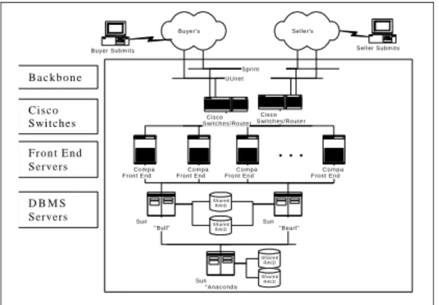
With the appropriate system model, it is possible to extend the results shown in the previous section to the system level. Figure 5 shows a simplified representation of the eBay Internet auction web site based on a description from the Los Angeles Times [Menn99]. The site is a 3-tier architecture consisting of dual redundant Internet Wide Area Networks (WANs), routers, the front-end PC servers describe above, and Database Management System (DBMS) servers.
UUnet Backbone Sprint Backbone Buyer Submits Bid Buyer's
ISP Seller'sISP
Seller Submits Item Cisco Mirrored Switches/Router s Cisco Mirrored Switches/Router s C o m p a q Front End Server C o m p a q Front End Server C o m p a q Front End Server C o m p a q Front End Server Sun
Starfire/DBMS"Bull" Shared SunStarfire/DBMS"Bearl"
RAID Shared RAID Sun Starfire/DBMS"Anaconda " . . . Shared RAID Shared RAID B a c k b o n e Cisco Switches F r o n t E n d Servers D B M S Servers
Figure 5. Simplified Diagram of 3-tiered e-Commerce Site [Menn99]
Figure 6 shows the hierarchy of a MEADEP model that represents this system. The top level block diagram (not shown here) has 4 elements in series: the Internet backbone WAN, the gateway subsystem (routers and switches), the server subsystem, and the DBMS. Each of these blocks is in turn decomposed into Markov models. The server subsystem and individual server models described above are shown in contrasting colors. A complete description of this model can be found in [Hecht01] Backbone Model (Markov) Gateway Model (Markov) Server (Markov) Server Subsystem (Markov) Hardware (Markov) Solaris_OS (Markov) Software (Markov) DBMS Server Block Dgm Top Level Model
(Block Dgm)
Figure 6. MEADEP hierarchical model representing Figure 5.
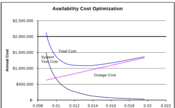
With the complete model, it is possible to perform a higher level of economic analysis in which software reliability growth can be traded off against any of the other 28 input parameters. A complete discussion of such tradeoffs is not possible within the scope of this paper. However, an example of such a result is shown in Figure 7. In this figure, the annual outage cost and. the testing cost (also assumed to be annually recurring based on continuous updates) are plotted against the total system failure rate. The system testing costs are assumed to be $1500 per hour and the outage time costs are assumed to be $25,000 per hour. Under these assumptions, the lowest total cost is achieved with a reward weighted failure rate is in the range of 0.01 to 0.015 (approximately 70 to 100 hour MTBF), and the total optimized annual cost related to availability (both test and outages) is approximately $1,000,000. Ths reward weighted failure rate integrates the impact of both degraded (i.e., reduced capacity) and full service operation and is a measure of performability. The unweighted failure rate, i.e., the probability that the site will be totally off-line rather than degraded, is 0.0012 per hour.
Availability Cost Optimization
$-$500,000 $1,000,000 $1,500,000 $2,000,000 $2,500,000 0.008 0.01 0.012 0.014 0.016 0.018 0.02 0.022
System Failure Rate (per hour, reward weighted)
Annual Cost
Total Cost
Outage Cost System
Test Cost
Figure 7. Availability Related Costs for the e-Commerce Example shown in Figure 5
5.
Discussion and Conclusions
This paper has demonstrated the value of integrating two mature and complementary, but until now, separated modeling and prediction approaches. As a result of this integration, it is possible to make better predictions on the economically achievable reliability of software intensive systems that incorporate redundancy and in which capacity and response time have economic value. As such the technique is also applicable to many classes of high assurance systems in space, air traffic
control, military information (e.g., C3I and logistics),
and manufacturing, financial, and medical applications. The model results should be interpreted with respect to the following limitations:
1. Software test data. As has been noted in many
articles and papers on the subject, proper data gathering is essential for the validity of such models. The test data that are used should be gathered in accordance with the anticipated operational profile [Musa96] and should reflect a variety of testing strategies to avoid test saturation.
2. Random failures: The “heisenbug” assumption
noted above assumes that failures occur randomly and can be modeled as a stochastic process. This is largely true even for software failures. Deterministic software failures are easily reproduced and generally fixed early. Those that are difficult to reproduce are by definition unpredictable and therefore non-deterministic. Because most failures in software, hardware, and communications system are random and are the largest contributors to system downtime, the modeling and decision making approach described
here is valid. However, the modeling approach does not address deterministic phenomena such as fundamental design flaws or security challenges that have been responsible for some high visibility recent outages at large web sites.
References
[ANSI92] “American National Standard, Recommended Practice for Software Reliability”, American National Standards Institute, ANSI/AIAA R-013-1992
[Bavuso85] S.J.Bavuso, P.L. Petersen, Care III Model Overview and User's Guide, NASA Technical Memorandum 86404, Langley Research Center, Hampton, VA, 1985
[Fisher00] Kal Raman, Sr. VP and CIO of drugstore.com as quoted by Susan E. Fisher,
“E-business redefines infrastructure needs”, Infoword,
January 7, 2000, available from www.infoworld.com
[Farr93] W.H. Farr and O.D. Smith, Statistic Modeling and Estimation of Reliability Functions for Software
(SMERFS) Users Guide, TR 84-373, Revision 3, Naval
Surface Warfare Center, Dahlgren Division, September, 1993
[Farr96] W.H. Farr, “Software Reliability Modeling
Survey”, in Software Reliabiltiy Engineering, M., Lyu,
ed., IEEE Computing Society Press and McGraw Hill, New York, 1996, Chapter 3
[Goyal87] A. Goyal and S. Lavenberg, "Modeling and analysis of computer system availability", IBM Journal of Research and Development, Vol 31, No. 6, November, 1987
[Hecht97], M. Hecht, D. Tang, and H. Hecht “Quantitative Reliability and Availability Assessment
for Critical Systems Including Software”, Proceedings
of the 12th Annual Conference on Computer Assurance,
June 16-20, 1997, Gaitherburg, Maryland, USA [Hecht01] M. Hecht, "Reliability/Availability Modeling, Prediction, and Measurement for e-Commerce and other Internet Information Systems", Proceedings of the 2001 Annual Reliability and Maintainability Symposium, Philadelphia, PA, USA, Jan 21-25, 2001.
[LaPrie96], J.C. LaPrie, Software Reliabiliy and Systems
Reliability, in Software Reliabiltiy Engineering, M.,
Lyu, ed., IEEE Computing Society Press and McGraw Hill, New York, 1996, Chapter 2
[Lee93] I. Lee, D. Tang, R.K. Iyer, and M.C. Hsueh, "Measurement-Based Evaluation of Operating System Fault Tolerance," IEEE Transactions on Reliability, pp. 238-249, June 1993.
[Littlewood80] B. Littlewood, “The Littlewood-Verrall Model for Software Reliabiltiy Compared with Some
Rivals”, Journal of Systems and Software, vol. 1, no. 3,
1980
[Menn99] Joseph Menn, “Prevention of Online Crashes in No Easy Fix”, Los Angeles Times, October 16, 1999, Section C, Page 1
[Metz00] J.G. Metz, “Managing E-Commerce for 100% Uptime”, Internet Week Learning Programs, May, 2000 [Rosin99], A. Rosin, M. Hecht, J. Handal, “Analysis of
Airport Reliability”, Proceedings of the 1999 Annual
Reliability and Maintainability Symposium, Washington DC, USA, Jan 18-21, 1999, p. 432
[Sahner96], R. Sahner, K. Trivedi, A. Puliafito, Performance and Reliability Analysis of Computer Systems, Kluwer Academic Publishers, 1996
[Sanders95] Center for Reliable and High-Perofrmance
Computing, UltraSAN User's Manual. University of
Illinois, available from www.crhc.uiuc.edu/UltraSAN [SoHaR00] MEADEP home page, http//:www.sohar.com/meadep
[Schneidewind96], N. Schneidewind, “Software
Reliability Engineering for Client Server Systems”,
Proc. 7th International Symp. on Software Reliabiltiy
Engineering (ISSRE), White Plains, New York, October, 1996, pp. 226-235
[Strauss99] Gary Strauss, “When Computers Fail”, USA Today, page 1A, December 7, 1999
[Tang95] D. Tang and M. Hecht, “Evaluation of Software Dependability Based on Stability Test Data” Proc. 11th Int. Symp. Fault-Tolerant Computing, Pasadena, California, June 1995
[Tang99] D. Tang, M. Hecht, A. Rosin, J. Handal,
“Experience in Using MEADEP”, Proceedings of the
1999 Annual Reliability and Maintainability Symposium, Washington DC, USA, Jan 18-21, 1999.
[Trivedi85] K. Trivedi, R. Geist, M., Smotherman, and J.B. Dugan, "Hybrid Modeling of Fault Tolerant
Systmes", Computers and Electircal Engineering, An
International Journal, vol. 11. no. 2, pp. 87-108, 1985 [Winter99] Richard Winter, “The E-Scalability Challenge”, Intelligent Enterprise, December 21, 1999, Volume 2 - Number 18
[Wattanapongsakorn00] N. Wattanapongsakorn and S. Levitan, "Integrating dependability analysis into the
real-time system design process", Proc. Annual
Reliability and Maintainability Symposium, pp.327-334, Washington, DC 2000.