Methods for Quantitative Risk Analysis for Travel Demand Model Forecasts
1 2 3 Thomas Adler* 4 RSG 5 55 Railroad Row 6White River Junction, VT 05001
7 802.295.4999 8 [email protected] 9 10 Michael Doherty 11 URS 12
1625 Summit Lake Drive
13 Tallahassee, FL 32317 14 850.574.3197 15 [email protected] 16 17 Jack Klodzinski 18 Florida's Turnpike/URS 19
Florida's Turnpike Headquarters
20 Ocoee, FL 34761 21 407.264.3819 22 [email protected] 23 24 Raymond Tillman 25 RT Consultancy 26 345 West 58th Street 27 New York, NY 10019 28 212.315.3566 29 [email protected] 30 31 32 *Corresponding Author 33 Word Count: 4,539 34
Figure Count: 6 @250each = 1,500
35
Table Count: 0 @250 each = 0
36
Total Count: 6,039
37 38
Paper Submitted: August 1, 2013
39 40
Key Words: Risk analysis, uncertainty, travel demand modeling, response surface methods, tolled express
41
lanes
Abstract 1
Travel demand forecasting models have played a critical role in transportation planning, supporting
2
the evaluation of policies, programs and projects that involve complex interactions between the activity
3
system and the transportation system. Both the state-of-the-art and the state-of-the-practice in travel
4
demand modeling have advanced considerably over the many decades since the original four-step model
5
structure was conceived. However, the models are not now, and never will be, perfect representations of
6
the systems they represent and so there are inevitably uncertainties around the forecasts that these models
7
generate. There are many applications in which the travel demand forecasts are important, for example, in
8
determining whether a given alternative is financially or technically feasible or meets some benefit
9
threshold. In these applications, uncertainties in the model forecasts may translate directly into risks of
10
not accomplishing the objectives related to the decision to implement or not implement the alternative.
11
For projects that involve outside financing, this threshold varies greatly between equity and lender
12
participants because of their differing risk-reward profiles.
13
Several previous papers and reports have described the uncertainties associated travel demand
14
forecasting and recommended ways of improving the state-of-the-practice. Among those
15
recommendations is the application of formal quantitative risk analysis methods. This paper summarizes
16
the existing literature and describes the application of one relatively straightforward but robust approach
17
for conducting quantitative risk analysis with travel demand forecasting models.
18
The formal risk analysis approach described here can assist by providing a more complete evaluation
19
of a project’s likelihood of achieving specified objectives. In addition, it can have a broader application
20
in the development of traffic and revenue forecasts other than a “most likely” or 50% probability of
21
attainment (“P50”) scenario. When another probability level or target is requested (e.g., 75% by a debt
22
provider or rating agency), traffic and revenue analysts can use expected values for many required inputs
23
and prepare a P50 forecast. They can then apply the procedures outlined here to determine the
24
probabilities of attaining other levels of demand or revenue.
25 26 27 28 29 30
INTRODUCTION
1
Travel demand forecasting models have played a critical role in transportation planning, supporting
2
the evaluation of policies, programs and projects that involve complex interactions between the activity
3
system and the transportation system (see, for example, 1). Both the art and the
state-of-the-4
practice of travel demand modeling have advanced considerably over the many decades since the original
5
four-step model structure was conceived. However, the models are not now, and never will be, perfect
6
representations of the road or transit systems they represent and so there are inevitably uncertainties
7
around the forecasts that these models generate.
8
In some travel demand modeling applications, such as those involving comparisons among project
9
alternatives, uncertainties in the absolute magnitudes of the forecasts may not be as important. For
10
example, the decision to be supported by travel demand forecasts may involve the relative position or
11
ranking of alternatives, one or more of which will be selected regardless of magnitude in the demand.
12
However, there are many other applications in which the absolute magnitudes of the forecasts are
13
important, for example, in determining whether a given alternative is financially or technically feasible or
14
meets some benefit threshold. With these applications, uncertainties in the model forecasts may translate
15
directly into risks of not accomplishing the objectives related to the decision to implement or not
16
implement the alternative. There are clearly many transportation planning applications of travel demand
17
models that fall into this latter category such as tolled express lanes for managed lanes projects.
18
Several previous papers and reports have described the uncertainties associated with travel demand
19
forecasting and recommended ways of improving the state-of-the-practice. Among those
20
recommendations is the application of formal quantitative risk analysis methods. This paper summarizes
21
existing literature and describes the application of one relatively straightforward but robust approach for
22
conducting quantitative risk analysis with travel demand forecasting models.
23
The formal risk analysis approach described here can assist by providing a more complete evaluation
24
of a project’s likelihood of achieving specified objectives. In addition, it can have a broader application
25
in the development of traffic and revenue forecasts other than a “most likely” or 50% probability of
26
attainment (“P50”) scenario. When another probability level or target is requested (e.g., 75% by a debt
27
provider or rating agency), traffic and revenue analysts can use expected values for many required inputs
28
and prepare a P50 forecast. They can then apply the procedures outlined here to determine the
29
probabilities of attaining other levels of demand or revenue.
30 31 32 33 34
BACKGROUND
35Concerns about the reliability of travel demand forecasts have been raised in a number of past studies.
36
The seminal, and often-cited, work of Pickrell (2) in the early 1990s focused attention on the large
37
differences between transit ridership forecasts that were developed for proposed new transit systems using
38
travel demand models and the actual ridership levels that were experienced after those systems were built.
His work indicated that the models’ ridership forecasts on average not only deviated significantly from
1
actual ridership but that the forecasts were systematically higher than actual ridership by a significant
2
margin. Other researchers have found similar effects both in the U.S. and internationally. Flyvbjerg (3)
3
reviewed a wider range of public works projects including both transit and toll road projects and found
4
both large and systematic gaps between model forecasts and actual usage. Bain’s work (see, for example,
5
6) focused on toll roads mirrors these other observations. Lemp and Kockelman (5) provide a
6
comprehensive review of risks and uncertainties in forecasting demand for toll road projects.
7
This past work has identified a number of reasons why forecasts are often quite different from actual
8
experience. These reasons generally fall into three categories:
9 10
1) Model structure and data – Travel demand forecasting models are at best simplifications 11
of the decisions that travelers make in response to transportation services and of the 12
response of the transportation system to those decisions (e.g., volume/delay relationships). 13
And, the data that are used to represent both the activity systems that generate demand and 14
the transportation system that carries that demand generally do not completely 15
characterize all of the details of those systems. While there has been considerable work 16
over the past several decades to improve these models and data, there is still much work 17
remaining to be done to address known limitations (see, for example, 6). 18
2) Analysis bias – The previously-cited studies of Pickrell, Flyvbjerg and Bain conclude that 19
the systematic over-prediction of travel demand for transit, toll road and other projects can 20
be explained in large part by a tendency of modelers to adopt overly-optimistic assumptions 21
with respect to the projects that they are evaluating. These can be attributed to factors 22
ranging from client pressure and deliberate misrepresentation of model results to a 23
sometimes unconscious “optimism bias”. 24
3) Inherent uncertainties in future conditions – Travel demand forecasting models include 25
projections of details of the study area’s activity and transportation systems into the future. 26
For example, population and employment projections are required at a relatively fine level 27
of geography – at a much higher granularity and often for a much longer time frame than 28
the U. S. Census or other commercial population and employment forecasting firms provide. 29
These projections can have significant effects on travel demand forecasts and yet we know 30
that the projections themselves are inherently uncertain, affected by factors such as 31
economic cycles which have similar associated uncertainties. 32
As a result of all these factors, it simply is not realistic to assume a single point forecast of travel
33
demand will be sufficient to make informative planning decisions where the magnitude of a demand
34
forecast determines if key objectives will be achieved. The factors above are related to uncertainties in the
35
direct inputs to the models, the structure of the models and the values of the model parameters, all of
36
which need to be considered in determining the levels of uncertainty associated with model outputs.
37
The need to formally consider uncertainties in forecasts has been recognized in the literature by many
38
others and quantitative methods for representing the uncertainties have been used in selected applications
39
such as energy consumption forecasting since at least the early 1970s (see, for example, 7). Lewis
provides a very articulate call for application of risk analysis in transportation planning and provides
1
examples of how it can be applied to cost estimation. (8)
2
While there have been only limited applications of comprehensive quantitative risk analysis to travel
3
demand forecasting, uncertainties in the forecasts have been represented in other ways. The most common
4
approach is to conduct sensitivity analysis in which key inputs and model assumptions are varied
5
individually and the full travel demand model is run to determine their effects on the forecast metrics of
6
interest. Sensitivity testing is routinely conducted with travel demand models and, for example, is
7
generally considered to be a key component of “investment grade” forecasting exercises for toll facilities.
8
These analyses provide valuable information about the models’ responses to key inputs and the potential
9
variability of forecasts. However, the levels of each variable tested are typically arbitrarily set and do not
10
necessarily correspond to any particular likelihood of occurrence. And, more importantly, sensitivity
11
analyses are typically conducted by varying only one variable at a time and thus interactions among these
12
variables are not represented.
13
Scenario testing, in which likely future conditions are described by a combined set of changes in
14
model inputs, is commonly used to test the interactive effects among two or more uncertain inputs. Often,
15
these are used to test a set of “optimistic” (upside) or “pessimistic” (downside) assumptions and they can
16
provide useful information about outcomes ranging from expected to extreme. They can also provide
17
some indication of risk and, in fact, are commonly used as stress tests in financial modeling. However,
18
running a small number of discrete scenarios cannot fully describe the range of outcomes or the relative
19
likelihoods of those outcomes and thus should not be considered a complete substitute for a full
20
quantitative risk analysis.
21
In concept, a full quantitative risk analysis involves a relatively straightforward two-step process:
22
1) Estimate the probability distributions of key model inputs and assumptions – There are 23
many model inputs and assumptions that could significantly affect model forecasts. These could
24
include, for example: land use patterns/distribution, employment, fuel cost and
25
environmental/regulatory constraints on future development. In some cases the modeler has data
26
that can be used to estimate both the shapes and parameters of the distributions of the key drivers.
27
For example, if survey data are used to estimate model parameters, the sampling error
28
distributions can be used for those parameters. Some state forecasting research agencies and
29
commercial firms that produce regional population and employment projections recognize these
30
uncertainties by publishing data on the magnitudes of their forecast errors over different time
31
horizons. Those data can similarly be used to estimate the probability distributions of those model
32
inputs. However, there are inevitably model inputs for which there are no data available to
33
describe likely ranges or distributions. For these cases, either the project team’s
34
subjective/professional judgment can be used to estimate distributions or a more formal approach
35
such as the Delphi Method (9) can be used. In either case, the assumptions are at least then
36
explicit and their effects on risk can be formally tested.
37
2) Estimate the probability distributions of the model outputs – Given the probability 38
distributions of the inputs and a model that uses those inputs to generate outputs, the distributions
39
of those outputs can be determined either analytically or, more commonly, using Monte Carlo
40
simulation. An analytical calculation is possible if the input distributions are relatively simple
41
(e.g., all independent uniform) and the model can be expressed in a relatively simple closed-form
42
(e.g., linear). However, these conditions are not generally met with travel demand forecasting
43
models and so some form of Monte Carlo simulation is typically required. Fortunately, excellent,
easy-to-use commercial and open-source packages are available to conduct Monte Carlo
1
simulation.
2
While this process is generally straightforward and has been applied to many other applications, its
3
direct application to typical travel demand forecasting models is computationally intractable. This is
4
because Monte Carlo simulations typically require thousands of random draws of the inputs to reliably
5
estimate output distributions, each requiring the model to be run to generate the outputs that correspond to
6
the inputs. Most regional travel demand forecasting models require hours or days to run and even a very
7
simple model that could run in minutes would require a significant Monte Carlo simulation runtime. Even
8
though computation speeds have been improving with faster computers and distributed processing, travel
9
demand models have increased in geographic resolution and complexity at rates that have offset these
10
computational speed improvements.
11
In addition to the approach that is described in more detail in this paper, at least four other approaches
12
have been used to support quantitative risk analyses of travel demand model forecasts.
13 14
1) Treating the inputs as independent effects – Simple univariate sensitivity tests with the 15
full travel demand forecasting model can be used to estimate how each variable individually 16
affects the outputs. The differences from base outputs can be represented as simple 17
deviations for each input and these differences, summed across all inputs, can be used in a 18
Monte Carlo simulation to represent forecasts for the combinations of changed inputs 19
represented by each set of Monte Carlo draws. The limitation of this approach is that it does 20
not address the often complex interactions among inputs that can make their combined 21
effects much different from the simple sum of their individual effects. 22
2) Bayesian melding – Sevcikova, Raftery and Waddell (10) used Bayesian melding with 23
Urbansim to efficiently generate posterior distributions of the outputs based on prior 24
distributions of inputs and data on outputs for selected years of the simulation. This 25
approach works well for this type of application in which data are available on outputs to 26
support the estimation of weights for the melding process. 27
3) Using a “structure and logic” version of the model – HDR and a predecessor firm, HLB, 28
have used an approach in which they create a separate, simplified, travel demand 29
forecasting model that represents the basic structure of the process that generates travel 30
demand, without the full complexity of a complete regional travel model (11). This model 31
can then be embedded in a Monte Carlo simulation to generate the distributions of outputs. 32
4) Simplifying the travel demand model – Zhao and Kockelman (12) were able to conduct 33
100s of runs to determine how errors propagated through four-step models by creating a 34
faster-running but otherwise equivalent version of the travel demand model that they were 35
using. They also noted that “… simple regressions of outputs on inputs offer very high 36
predictive power, suggesting that prime sources of forecast uncertainties can be rather quickly 37
deduced – and exploited – for better prediction.” 38
All of these approaches represent ways of quantifying the likelihood of different model outcomes
39
given uncertainties in the model structure, parameters and inputs. The first two listed are relatively
straightforward and can be done with little additional effort, though Bayesian melding does require
1
longitudinal data that are not commonly compiled for travel demand models. The second two approaches
2
both require additional modeling work and potentially a fair amount of effort; creating and validating a
3
new parallel “structure and logic model” or creating a more computationally-efficient version of the
4
original travel demand, retaining its structure.
5
The approach that is detailed in this paper follows from observations similar to those of Zhao and
6
Kockelman; most notably, that closed-form models can be created using multivariate statistical analysis
7
that very closely approximates the behavior of the much more complex and computationally demanding
8
regional travel demand forecasting models. The need to create an analytically-tractable representation of a
9
complex process is common in laboratory sciences and engineering and response surface methods have
10
been developed to efficiently and effectively fill that need (13).
11
Response surface modeling uses statistically-efficient experiments and a variety of statistical methods
12
are used to create models describing the relationships between process (model) inputs and outputs. In this
13
application, the experiments are simply combinations of travel demand model inputs, constructed in ways
14
that support the statistical estimation of models which describe the relationship between the original
15
model’s inputs and outputs. Note that these resulting “synthesized” models are not equivalent to
16
“structure and logic” models in that: a) they are direct statistical derivatives of the full travel demand
17
models in respect to the relationships between selected inputs and outputs and b) they cannot be created
18
without first having a full travel demand model.
19
Figure 1 shows conceptually how response surface analysis can be used to support quantitative risk
20
analysis around travel demand forecasts.
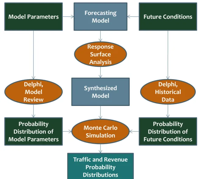
Figure 1 - Quantitative Risk Analysis Using Response Surface Methods 1
Forecasting
Model
Synthesized
Model
Probability
Distribution of
Model Parameters
Model Parameters
Probability
Distribution of
Future Conditions
Response
Surface
Analysis
Future Conditions
Monte Carlo
Simulation
Delphi,
Historical
Data
Delphi,
Model
Review
Traffic and Revenue
Probability
Distributions
2In this schematic, the forecasting model is a regional travel demand model or whatever model is used
3
to create the desired travel demand forecasts. There are uncertainties in the model parameters and
4
structure as indicated in the boxes on the left side of this figure and uncertainties in inputs such as future
5
conditions and other data as indicated on the right side of the diagram. Probability distributions can be
6
developed for all of these uncertain factors using the approaches described previously. The travel demand
7
forecasting model can be “synthesized” using response surface methods into an analytically-tractable
8
model that can then be imbedded in a Monte Carlo simulation to generate distributions of the outputs of
9
interest.
10
The following section describes one of the applications of this approach to travel demand forecasting
11
that authors of this paper have completed over the past several years.
12
THE ORLANDO I-4 EXPRESS LANES APPLICATION
13
Florida’s Interstate 4 connects the Tampa Bay and Daytona regions through the Orlando region in
14
Central Florida. Several factors, including the significant growth of the Orlando region, have led to
15
correspondingly high growth in I-4 traffic through the Orlando region. And, that growth has led to a need
to increase capacity of this highway section, which currently consists of four mainline lanes in each
1
direction. Florida DOT developed a plan for a managed lanes corridor through the Orlando area. The
2
plan adds two dynamically-tolled express lanes in each direction for a 21-mile section of the I-4 corridor.
3
Figure 2 shows the proposed project location in red. Other existing and proposed tolled facilities are
4
shown in green and brown.
5
Figure 2 - I-4 Managed Lanes Study Corridor (Source: 14)
6 7
8 9
A planning-level study was undertaken to evaluate the traffic and revenue that could be expected for
10
the proposed managed lanes (14). A relatively detailed travel demand modeling process was used for the
11
study, employing a four-step regional travel demand forecasting model paired with a more detailed
12
corridor-specific macroscopic simulation model. Initial sensitivity analyses indicate that population
growth rates, estimated values of time, completion of other network capacity enhancements and toll rates
1
were key drivers of the model’s forecasts. The first three of these represent uncertain model inputs and
2
toll rates are policy variables that can be controlled by the facility owner/operator.
3
Because toll revenues will provide an important part of the project’s funding, traffic and revenue
4
estimates were desired to represent levels that would be met or exceeded with a probability of 0.75. This
5
corresponds with a relatively risk-averse position, providing some assurance that the projected revenues
6
would most likely be realized, as compared to more typical “expected values” which would theoretically
7
represent over-estimates 50% of the time.
8
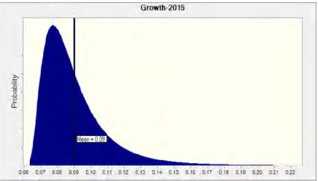
The first step of the process was to develop probability distributions for each of the three key
9
uncertain inputs. Projected population growth rates for the Orlando area and Florida as a whole changed
10
significantly after the most recent recession. Baseline population forecasts for the region were derived
11
from projections developed by the Bureau of Economic and Business Research (BEBR) at the University
12
of Florida. BEBR has several decades of experience producing forecasts for Florida counties and has
13
published reports described its forecasting accuracy over different projection horizons and also considered
14
the recent economic downturn with forecast adjustments. This information was used to estimate
15
probability distributions around the current estimates for each of the forecast years. Figure 3 shows an
16
example study area population growth probability distribution through the year 2015.
17
Figure 3 - Example Input Distribution for Population Growth to 2015 (fractional increase over 2010)
18
19
Values of time were estimated using data from travel surveys and the associated sampling error
20
distributions were used to provide probability distributions for these estimates. Finally, the likelihoods of
21
completing various other network capacity enhancements were subjectively estimated based on input
22
from Florida DOT planning engineers.
23
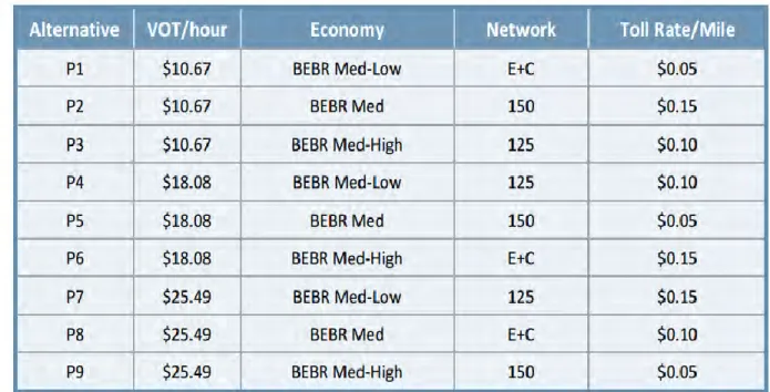
The response surface modeling used a relatively simple fractional factorial experimental design for
24
the travel demand model runs. Nine different run conditions were specified, run for each of seven forecast
25
years (five-year increments through 2045). Figure 4 shows these nine conditions (14).
Figure 4 - I-4 Managed Lanes Study Experimental Design
1
2
Value of time was varied in three levels and the economy (population growth) was similarly varied
3
with three levels, representing BEBR’s medium-high, medium and medium-low projections. Completion
4
of other roads in the Orlando network, some of which could divert traffic from the facility and others of
5
which could provide feeder capacity, was represented by existing plus committed project (E+C), those
6
projects needed to keep all major roads in the network at a volume to capacity ratio below 1.5 (150) and
7
those necessary for volume capacity ratios below 1.25 (125). Finally, daily average toll rates were varied
8
in the regional model between $0.05/mile and $0.15/mile.
9
The response surface modeling used data from these runs to determine the functional form that best
10
fit the observed model response patterns. The resulting models are nonlinear in the variables but
linear-in-11
the-parameters and so could be easily estimated with standard statistical software. As observed by Zhao
12
and Kockelman in their work, these simple statistical models fit the data very closely (R2 ~ 0.98), 13
suggesting that the synthesized models capture the original travel demand model’s behavior very closely
14
in these dimensions. Figure 5 shows an example model developed for I-4 traffic volumes; similar models
15
were also generated for toll revenues (14).
Figure 5 - Example I-4 Response Surface Model 1 2
yearCon
road
roadEC
rampUp
VOT
tollRate
growth
Traffic
150
*
15820
*
11099
)
ln(
*
9432
)
/
(
*
91138245
*
48486
128686
Where: Trafficis the number of daily one-way trips that use the I-4 Express Lanes
growthis the ratio of dwelling units in the given year to dwelling units in 2010 minus one
tollRateis the average toll rate charged on I-4 in 2010 $
rampUpis the number of years the project has been operating in the given year
roadECrepresents the road improvements included only in the E+C conditions
road150 represents an improvement program that maintains all roads below V/C of 1.5
yearConis a vector of constants representing the years for which the forecasts are
being made
3
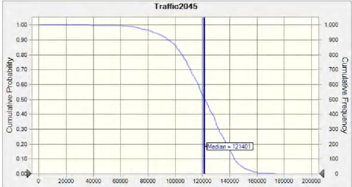
The response surface models were programmed along with the estimated distributions of the inputs in
4
a Monte Carlo simulation. The simulation was run with between 100,000 and 1,000,000 draws to estimate
5
the distributions of selected outputs. Figure 6 shows the reverse cumulative distribution output from one
6
of the simulation runs.
7
Figure 6 - Example I-4 Traffic Distribution (average daily traffic)
8
9
Models were developed for each of the project’s build scenarios and the simulations were used to
10
develop traffic and revenue distributions. These distributions showed the requested 75th percentile values, 11
along with all other percentile values.
12 13
CONCLUSIONS AND RECOMMENDATIONS
1
Travel demand forecasting models are not now, and never will be, perfect representations of the
2
systems that they represent and so there are inevitably uncertainties around the forecasts that these models
3
generate. The uncertainties derive from model structure, parameter estimates associated with the structure
4
and data including forecasts of inputs to the models. Many if not most of these uncertainties are inherent
5
in the modeling process and create risks associated with projects or programs which are supported by the
6
models’ forecasts. So, it is important to recognize those uncertainties in some way. Past studies have used
7
a variety of approaches to represent the uncertainties and risks, including simple sensitivity and scenario
8
analyses. However, those approaches do not fully quantify the levels of uncertainty in the forecasts.
9
There have been some applications of more formal quantitative risk assessment for travel demand and
10
land use forecasting models, also using a variety of approaches. This paper details one approach that can
11
be used with any travel demand forecasting model system, that does not require any calibration data
12
beyond that used for the development of the original travel demand model system and that directly
13
mirrors the behavior of that system while being computationally tractable when imbedded in a Monte
14
Carlo process. The formal risk analysis approach described here can assist by providing a more complete
15
evaluation of a project’s likelihood of achieving specified objectives. In addition, it can have a broader
16
application in the development of traffic and revenue forecasts other than a “most likely” or 50%
17
probability of attainment (“P50”) scenario.
18
The prevalence of uncertainties in travel demand forecasting, the risks that can be presented by those
19
uncertainties and the availability of approaches for quantifying those risks together present a compelling
20
case for more frequent applications of formal risk analysis in travel demand forecasting.
21 22
REFERENCES
23
1. Manheim, M. L. Fundamentals of Transportation Systems Analysis. MIT Press, Cambridge, MA, 24
1979. 25
2. Pickrell, D.H. “A Desire Named Streetcar: Fantasy and Fact in Rail Transit Planning.” Journal of 26
the American Planning Association, Vol. 58, pp.158-176, 1992. 27
3. Flyvbjerg, B., M. K. S. Holm, and S. L. Buhl (2005). How (In)Accurate Are Demand Forecasts in 28
Public Works Projects? The Case of Transportation.” Journal of the American Planning 29
Association, Vol. 71 (2), pp. 131–146, 2005. 30
4. Bain R. “Error and Optimism Bias in Toll Road Traffic Forecasts.” Transportation, Vol. 36, No. 5, 31
2009. 32
5. Lemp, J. and K. M. Kockelman. “Understanding and Accommodating Risk and Uncertainty in Toll 33
Road Projects: A Review of the Literature.” Transportation Research Record: Journal of the 34
Transportation Research Board No. 2132, Transportation Board of the National Academies, 35
Washington, D.C., 2009, pp. 106-112. 36
6. Committee for Determination of the State of the Practice in Metropolitan Area Travel 37
Forecasting. Special Report 288: Metropolitan Travel Forecasting Current Practice and Future 38
Direction. Transportation Board of the National Academies, Washington, D.C., 2009. 39
7. Salter, R. G. A Probabilistic Forecasting Methodology Applied to Electric Energy Consumption. 40
Report R-993-NSF, Rand Corporation, Santa Monica, CA, 1973. 41
8. Lewis, D. “The Future of Forecasting: Risk Analysis as a Philosophy of Transportation Planning.” 1
Transportation Research News 177. Transportation Research Board of the National Academies, 2
Washington D. C., 1995. 3
9. Dalkey, N. and O. Helmer. An Experimental Application of the Delphi Method to the Use of Experts. 4
Memorandum RM-727/1-Abridged, Rand Corporation, Santa Monica, CA, 1962. 5
10. Sevcikova,H., A. E. Raftery and P. A. Waddell. “Assessing Uncertainty in Urban Simulations Using 6
Bayesian Melding.” Transportation Research Part B: Methodological, Vol. 41, pp. 652-669, 2007. 7
11. HDR. Toll Road Modeling Support: Final Report. Prepared for Maricopa Association of 8
Governments, Phoenix, AZ, 2012. 9
12. Zhao, Y. and K. M. Kockelman. “The Propagation of Uncertainty Through Travel Demand Models: 10
An Exploratory Analysis.” Annals of Regional Science, Vol. 36, No. 1, 2002, pp. 145-163. 11
13. Meyers, R. H., D. C. Montgomery and C. M. Anderson-Cook. Response Surface Methodology. John 12
Wiley & Sons, Hoboken, NJ, 2009. 13
14. URS Corporation. Technical Memorandum Planning-Level Traffic and Revenue Study Interstate 4 14
Tolled Managed Lanes, Prepared for Florida DOT, October 2012. 15
15. Bureau of Economic and Business Research. Special Report Number 9. University of Florida, 16
Gainesville, FL, July 2011. 17