World Maritime University
The Maritime Commons: Digital Repository of the World
Maritime University
World Maritime University Dissertations Dissertations
2000
A cash flow analysis approach to privatisation : case
study of Klaipeda Stevedoring Company
Andrius Saveikis World Maritime University
WORLD MARITIME UNIVERSITY
Malmö, Sweden
A CASH FLOW ANALYSIS APPROACH TO
PRIVATISATION: CASE STUDY OF KLAIP
Ė
DA
STEVEDORING COMPANY
By
ANDRIUS SAVEIKIS
Lithuania
A dissertation submitted to the World Maritime University in partial
fulfillment of the requirements for the award of the degree of
MASTER OF SCIENCE
In
PORT MANAGEMENT
2000
DECLARATION
I certify that all the material in this dissertation that is not my own work has been identified, and that no material is included for which a degree has previously been conferred on me.
The contents of this dissertation reflect my own personal views, and are not necessarily endorsed by the University.
(Signature) ...
(Date) ...
Supervised by:
Name: Prof. Patrick Donner
Office: Associate Professor, Shipping Management Institution/organization: World Maritime University
Assessor:
Name: Prof. Shuo Ma
Office: Course Professor, Port- and Shipping Management
Institution/organization: World Maritime University
Co-assessor:
iii
ACKNOWLEDMENTS
I take this opportunity to express my sincere gratitude and indebtedness to my sponsors the European Community, for their generous fellowship that has enabled me to undertake my studies at the World Maritime University.
My special thanks go to my supervisor Professor Patrick Donner for his patience and encouragement in completing this paper.
Equally, I would like to extend my thanks to my course professors Shuo Ma, Bernard Francou and all other professors and lecturers as well as visiting professors for all their advice, directives and sharing of immense knowledge and experience.
Special appreciation to the Klaipėda Stevedoring Company for providing material for the research.
I also show my gratitude to all PM students and my friends whose friendship and corporation enriched my life in Malmö and gave me a good memory.
ABSTRACT
Title of Dissertation:
A cash flow analysis approach to privatisation: a case study of Klaipėda Stevedoring Company
Degree:
MSc. In Port Management
This dissertation focuses on the financial resource management, and in particular, cash flow management.
The research is based on a case study of Klaipėda Stevedoring Company and it covers a three year period when the company was preparing for privatisation.
The author looks at the cash flow statements and tries to assess which of the areas of activity are most significant to the company’s cash flow.
The changes in the amount of inventory, the credit given to customers or taken from suppliers and its impact on cash flow are examined.
The relationship between the current assets and current liabilities are explored by looking at movements that have taken place within the working capital of the firm. For a better view, time factor was considered in a cash cycle, and assessment of the efficiency of the company’s credit policies was analysed.
This analysis helps to see how the company was managing its cash flows through investment in inventory, credit provided to customers and credit taken from suppliers. The faster cash circulation through the business the lower is the amount of the capital tied up in operating assets and, as every time the cash completes the circuit a profit is taken, the higher is the rate of return achieved.
v
TABLE OF CONTENTS
Declaration ii
Acknowledgements iii
Abstract iv
Table of Contents v
List of Tables ix
List of Figures xi
List of Abbreviations and Symbols xii
1 Introduction 1
1.1 The aim and scope of the study 1 1.2 Methodology and encountered difficulties 2
1.3 Structure of the dissertation 4
2 Changes in the cash position of the company 5
2.1 Introduction 5 2.2 The statement of cash flow 6 2.2.1 Cash flow from operating activities 7 2.2.2 Cash flow from investment activities 11
2.2.3 Cash flow from financing activities 12 2.2.3.1 The company’s self financing capability 14 2.2.4 Cash flow from extraordinary activities 15 2.3 Changes in cash balances 16
3 Working capital analysis 19
3.1 Introduction 19 3.2 Current Assets 20 3.2.1 Cash and equivalents 20 3.2.2 Short-term investments 21
3.2.3 Accounts receivable 22 3.2.4 Inventories 24 3.2.5 Changes in the current assets 25 3.3 Current liabilities 25 3.3.1 Trade creditors 26 3.3.2 Taxes, remuneration and social security costs 27 3.3.3 Other amounts payable 28 3.3.4 Changes in the current liabilities 28 3.4 Changes in the working capital 29 3.4.1 Working capital to sales ratio 30
3.5 Conclusions 31
4 Changes in the liquidity of the company 32
4.1 Introduction 32 4.2 Current ratio 33
4.3 Quick ratio 34
4.4 Cash and short term investments to the total
current liabilities ratio 36
vii
5.4 Accounts receivable cycle 46 5.5 Accounts payable cycle 47 5.6 Trade debtors to trade creditors ratio 48 5.7 The cash cycle 49
5.8 Conclusions 51
6 Funds flow statement analysis 53
6.1 Introduction 53 6.2 Sources of funds 54 6.3 Uses of funds 55 6.4 The funds flow statement 56 6.4.1 Changes in the company’s assets in general 56 6.4.2 Changes in the company’s long-term assets 57 6.4.3 Changes in the company’s short-term assets 58 6.4.4 Changes in equity and liabilities 59 6.4.5 Changes in the capital and reserves 60 6.4.6 Changes in long-term and short-term liabilities 62 6.5 Comparison of sources and uses of funds 63
6.6 Conclusions 64
7 Conclusions 65
7.1 Overview of the study 65 7.2 Assessment of the financial resource management in
the company 66
7.2.1 Assessment of the company’s cash position 69 7.2.2 Assessment of the company’s need for working
capital 70
References 72
Appendices 74
Appendix 1 Form of the cash flow statement 74
ix
LIST OF TABLES
Table 2.1 Net cash flow from operating activities (1996-1998) 8 Table 2.2 Cash flow from investment activities (1996-1998) 11
Table 2.3 Cash flow from financing activities (1996-1998) 13 Table 2.4 Self-financing ratio (1996-1998) 14 Table 2.5 Changes in cash balances (1996-1998) 16 Table 3.1 Short-term investments (1996-1998) 22 Table 3.2 Changes in accounts receivable (1996-1998) 23 Table 3.3 Changes in inventories level (1996-1998) 24 Table 3.4 Changes in the trade creditors level (1996-1998) 26 Table 3.5 Changes in the taxes, remuneration and social
security level (1996-1998) 27 Table 3.6 Changes in the other amounts payable (1996-1998) 28 Table 3.7 Changes in the working capital of the company (1996-1998) 30 Table 3.8 Working capital to sales revenue ration (1996-1998) 30 Table 4.1 Changes in the current ratio (1996-1998) 34 Table 4.2 Changes in the inventory holding level (1996-1998) 35 Table 4.3 Changes in the quick ratio (1996-1998) 35 Table 4.4 Increase in trade debtors (1996-1998) 37 Table 5.1 Average daily sales and costs (1996-1998) 41
Table 5.8 The cash cycle (1996-1998) 50 Table 5.9 The company’s need for the working capital (1996-1998) 51
Table 6.1 Changes in the company’s assets (1997-1998) 56 Table 6.2 Changes in long-term assets (1997-1998) 58 Table 6.3 Changes in short-term assets (1997-1998) 59 Table 6.4 Changes in equity and liabilities (1997-1998) 60 Table 6.5 Changes in capital and reserves (1997-1998) 61
xi
LIST OF FIGURES
LIST OF ABBRIVIATIONS AND SYMBOLS
ADC Average daily costs ADS Average daily sales d. Day/days
KLASCO Klaipėda Stevedoring Company
Lt. Litas, currency of the republic of Lithuanian USD Dollar, currency of the United States of America --- No data; illogical
CHAPTER 1
Introduction
1.1. The aim and scope of the study
Globalisation and privatisation processes, which have taken place during the last decade, have led to increasingly fierce competition in the port industry throughout the world. As a result, they have added tremendously to the pressure on port managers who face a continuous challenge of enhancing and sustaining their organisations’ competitive advantage.
Traditionally, to deal with competition, port managers focused their attention on operational performance, neglecting another very important side of business management - finance. However, the financial resources management could also make a difference and be an effective tool in striving to attain a competitive advantage.
Partially this is true. Nevertheless, the changing business environment requires port managers to have an integrated knowledge and skills and therefore the ability to understand, interpret and use the information provided in financial statements.
The author of this dissertation focuses on one particular aspect of financial resources management, that is cash flow management.
Cash flow is a very important financial concept. Every activity of any company is translated into cash at some time. Cash is used to pay employees and suppliers, to make investments into assets, pay dividends to providers of financial resources and for many other purposes. No business can continue once it has an insufficient cash balance. However, too much cash, as an idle resource, might be wasteful and indicate that the company is not operating as profitably as it could be.
Therefore, understanding and managing cash flows in a proper way not only could allow a company to survive, but also allow it to increase its profitability and achieve the flexibility needed to take advantage of unexpected business opportunities, hence increasing its competitive potential.
This dissertation is based on an analysis of the cash flows in Klaipėda Stevedoring
Company (hereinafter referred to as KLASCO).
KLASCO is the biggest stevedoring company in Lithuania. Having monopolised the market for a long time as a state corporation, it handles more than fifty percent of the
3
1999 and remains the only developed specialised container terminal on the eastern
coast of the Baltic Sea.
It is the author’s conviction that this research is a unique opportunity to show how the financial resource management could change a business situation. For this purpose the author has chosen a very dramatic and exciting moment in the life of the company during its preparation for privatisation. The company was privatised at the
beginning of 1999.
1.2. Methodology and encountered difficulties
This dissertation is a case study of cash flow management in Klaipėda Stevedoring
Company covering a three-year period before privatisation (1996-1998). The study
has been developed through the analysis of the financial statements collected from the company.
In addition to materials collected from the company, the author made research from journals, periodicals, books and Internet sources. Data was also collected from seminars and lectures conveyed at the World Maritime University as well as oral interviews from relevant persons during field studies. Computer spreadsheets were used where necessary to make comparisons and trend analyses of statistical data.
companies because of the differences in their functional responsibilities and financial structures.
1.3. Structure of the dissertation
Chapter 1 is a general introduction of the study. Here the author presents his view about the importance of financial resource management in attaining a competitive advantage and defines the area, scope and methodology of the analysis.
As a starting point for assessing the company’s financial situation before privatisation, the author looks at the company’s cash balances between the years
1996 and 1998 and examines changes occurring in that period. This is covered in
Chapter 2.
Chapter 3 tries to get a better view of the company’s financial position by expanding the scope of analysis to cover all current assets and current liabilities. A look is taken at the changes in what is commonly called the working capital of the company.
Chapter 4 assesses the changes in the company’s liquidity.
The adequacy of the company’s credit policies is considered in analysing the cash cycle in Chapter 5.
5
CHAPTER 2
Changes in the cash position of the company
2.1. Introduction
As a starting point for assessing changes in the financial position of the Klaipėda
Stevedoring Company before privatisation, we will look at the amounts of cash held by
the company in the period between the years 1996 and 1998. For the purpose of the
financial analysis we define the term cash as all money and bank balances which the company had readily available for immediate use.
We will examine what has happened to the firm’s cash resources during that time and will look at different factors which affected the situation. In particular we will concentrate our attention on cash generated from operations, strategic cash outflows for investments, and the external financing of the company. In order to do that we will compare three cash flow statements representing the mentioned period.
An examination of the cash balances of the enterprise will provide us with the initial insight into the privatisation of the company and will lay grounds for the better understanding of these particular actions and steps which were undertaken by the management at that time.
Now let us walk through the company’s cash flow statement.
2.2. The Statement of Cash Flows
The cash flow statement tracks the movement of cash through the business over a period of time. It records all the company’s transactions that use cash or supply cash. It shows:
• cash on hand at the start of a period;
• cash received in the period;
• cash spent in the period;
• cash on hand at the end of the period.
Typically, the cash flow statement is divided into sections with cash flows shown according to the activity giving rise to them. According to the accounting regulations passed by the Supreme Council, the Government and the Ministry of Finance of the Republic of Lithuania, all cash movements are classified under four main headings (see
Appendix 1):
• Cash flow from operating activities;
• Cash flow from investing activities;
7
At the end of the statement there is a section which indicates changes in the cash held position and shows cash at the beginning and at the end of the financial period.
2.2.1. Cash flow from operating activities
Cash flow from operating activities is the main indicator of the business. It enables the enterprise to compare its maintenance and development level to its working capacity. It shows the company’s ability to cover debts, pay out dividends, and make investments from its own sources. In another words - it allows us to follow the cash involved in the company's core business operations.
During the preparation of the cash flow statement, cash flow from operating activities is calculated by adjusting the current year result (profit or loss) with the following amounts (see Table 2.1):
• the influence of non-monetary items on tangible long-term assets, amortisation of
intangible assets, changes in stocks, changes in the amount of provisions, changes in the exchange rates, and so on. (according to the regulations if the amounts of the items mentioned above are small, they are joined into one item Depreciation and amortisation expenses);
• the influence of changes in amounts payable and receivable involving settlements
with clients and suppliers;
• the influence of taxes and other amounts payable to the Government budget;
• the influence of changes in prepayments;
• the result from financial and investment activities, because these activities are
reflected separately in appropriate items.
where the income statement had deducted it, and vice versa for a negative number. The bottom-line result is net cash from operations.
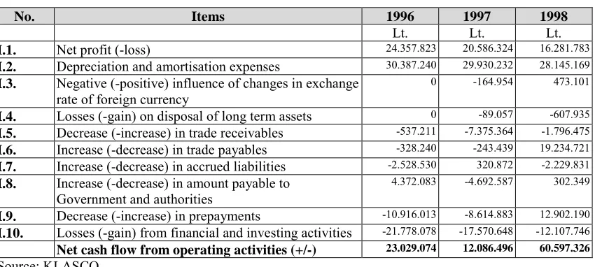
Table 2.1: Net cash flow from operating activities (1996 - 1998)
No. Items 1996 1997 1998
Lt. Lt. Lt.
I.1. Net profit (-loss) 24.357.823 20.586.324 16.281.783
I.2. Depreciation and amortisation expenses 30.387.240 29.930.232 28.145.169 I.3. Negative (-positive) influence of changes in exchange
rate of foreign currency
0 -164.954 473.101
I.4. Losses (-gain) on disposal of long term assets 0 -89.057 -607.935
I.5. Decrease (-increase) in trade receivables -537.211 -7.375.364 -1.796.475 I.6. Increase (-decrease) in trade payables -328.240 -243.439 19.234.721 I.7. Increase (-decrease) in accrued liabilities -2.528.530 320.872 -2.229.831 I.8. Increase (-decrease) in amount payable to
Government and authorities
4.372.083 -4.692.587 302.349
I.9. Decrease (-increase) in prepayments -10.916.013 -8.614.883 12.902.190 I.10. Losses (-gain) from financial and investing activities -21.778.078 -17.570.648 -12.107.746
Net cash flow from operating activities (+/-) 23.029.074 12.086.496 60.597.326
Source: KLASCO
Note: All the financial data is provided in the national currency litas (Lt.). Exchange rate 4 Lt. = 1 USD.
As we can see from Table 2.1 the company had a very unstable net cash flow from
operating activities. In the year 1996 net cash flow was 23 million Lt., in 1997 only 12
millions, but in 1998 it increased and was more than 60 million Lt.. These numbers seem
to be a little bit odd because the level of cash directly generated by the operations of the company (it is expressed in the net profit without any deduction for depreciation and represents a rough indication of the cash flow being generated by the enterprise during
9
Figure 2.1: Net profit without deduction for depreciation (1996-1998)
Source: KLASCO
In order to understand why there was such a big difference between the result in the
years 1996, 1997 and 1998 we have to look at net cash flow from operating activities a
little bit closer.
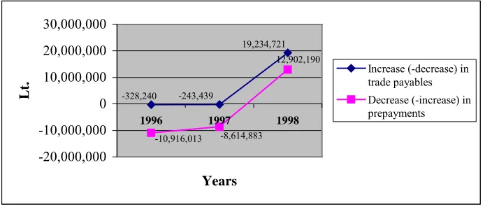
First of all what we can see is a huge change in the trade payables area (see Figure 2.2).
During the year 1998 it increased by more than 19 million Lt..
Figure 2.2: Changes in trade payables and prepayments (1996-1998)
Source: KLASCO
-328,240 -243,439
19,234,721 12,902,190
-10,916,013 -8,614,883
-20,000,000 -10,000,000 0
10,000,000 20,000,000 30,000,000
1996 1997 1998
Years
Lt.
Increase (-decrease) in trade payables Decrease (-increase) in prepayments 44,426,952
50,516,556 54,745,063
30,000,000 40,000,000 50,000,000 60,000,000
1996 1997 1998
Years
Lt
. Net profit without
Second, there was an even bigger change in the prepayments area (Figure 2.2). They
decreased. The difference between the year 1997 and the last year before the
privatisation (1998) was almost 20 million Lt..
Combined together these changes allowed the company to free around 40 millions of cash from operating activities.
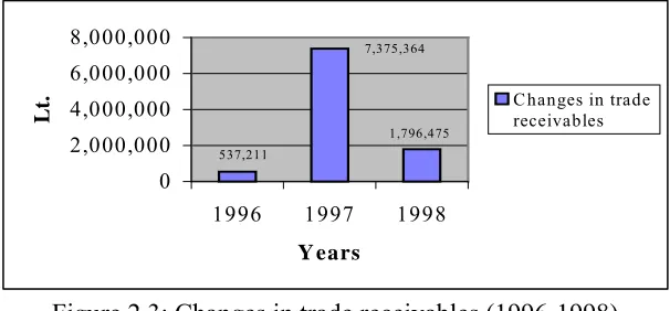
This indicates that it must been a shift in the company’s credit policy in 1998. The
assumption is also supported by another point - the change in the level of trade receivables (see Figure 2.3).
Figure 2.3: Changes in trade receivables (1996-1998)
Source: KLASCO
However, in that case we have to agree that it is difficult to distinguish a stable pattern of cash flows because the situation has changed every year. Nevertheless, the decrease in trade receivables amounts shows that the company probably has tightened its control in that area.
537,211
1,796,475 7,375,364
0 2,000,000 4,000,000 6,000,000 8,000,000
1996 1997 1998
Y ears
Lt
. Changes in trade
11
2.2.2. Cash flow from investment activities
Investment activities are second in importance to operating activities. They usually involve large amounts of money and represent strategic cash outflows paid in the current period that will earn revenue in forthcoming periods. Cash flow from investment activities include:
• cash paid in acquiring tangible and intangible long-term assets;
• cash paid for acquiring various securities;
• cash received from disposal of tangible and intangible long-term assets (except for
assets purchased for resale);
• cash received from sales of securities (except for securities purchased for resale).
According to the Lithuanian accounting regulations the item Cash flow from disposal of
investments also reflects dividends received by the enterprise during the accounting
period. If the latter is significant - it could be reported separately (Pačiolis, 1995, p. 95).
Table 2.2 shows how much the company has spent on capital expenditures in our analysed period. These were investments that KLASCO was making for the purpose of
building its business. As we can see, especially big expenses were made in the year 1998
(line II.1.).
Table 2.2: Cash flow from investment activities (1996 - 1998)
No. Items 1996 1997 1998
Lt. Lt. Lt.
II.1. Sales (-purchases) of long-term assets -38.850.401 -17.728.729 -106.131.962
II.2. Sales (-purchases) of investments -5.994.582 8.000.000 -1.051.096
Net cash flow from investment activities (+/-) -44.844.983 -9.728.729 -107.183.058
The problem with the cash flow statement is that it indicates only the total amounts spent on fixed assets but does not disclose in any detail where or on what the cash was spent. However, we know that during the analysed period a new container terminal was built.
The construction of it started on November 21st, 1997. The terminal entered into service
on January 22nd, 1999. The information about this event is disclosed in the company’s
Internet web site (www.klasco.lt). It explains the large cash outflows in the year 1998.
Items in line II.2 are simply movements of cash and represent money paid for acquiring and selling various securities. Such movements of cash are not as significant as the capital expenditures. Therefore, we are not going to analyse them in more detail.
2.2.3. Cash flow from financing activities
The third section of the cash flow statement is financing activities. It includes:
• cash received from owners for issuing all types of shares and capital securities;
• cash received from creditors, from issuing bonds, bills of exchange and other
securities;
• cash received from credit institutions, when the company’s debts increase;
• other cash received from the enterprise’s financial activities (e.g. interest received);
• cash paid to owners in the form of dividends; cash paid to owners for repurchase of
shares;
• cash paid to credit institutions for interest accrued and repayment of loans;
• cash paid to other companies;
13
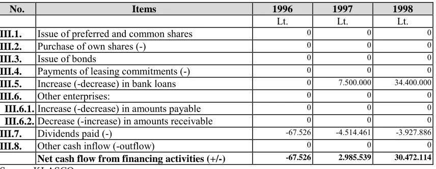
Table 2.3: Cash flow from financing activities (1996 - 1998)
No. Items 1996 1997 1998
Lt. Lt. Lt.
III.1. Issue of preferred and common shares 0 0 0
III.2. Purchase of own shares (-) 0 0 0
III.3. Issue of bonds 0 0 0
III.4. Payments of leasing commitments (-) 0 0 0
III.5. Increase (-decrease) in bank loans 0 7.500.000 34.400.000
III.6. Other enterprises: 0 0 0
III.6.1.Increase (-decrease) in amounts payable 0 0 0
III.6.2.Decrease (-increase) in amounts receivable 0 0 0
III.7. Dividends paid (-) -67.526 -4.514.461 -3.927.886
III.8. Other cash inflow (-outflow) 0 0 0
Net cash flow from financing activities (+/-) -67.526 2.985.539 30.472.114
Source: KLASCO
This is probably the least significant of the three analysed sections, because a business rarely receives cash from these sources more than once or twice a year. Nevertheless it provides some interesting information.
As we can see from table 2.3, starting in the year 1997 the company was using external
financing to support its activities. During the year 1998 the size of the loans increased
dramatically, they went from 7,5 to 34,4 million Lt. (see Figure 2.4).
Figure 2.4: Increase in bank loans (1996-1998)
Source: KLASCO
0 7,500,000 34,400,000 0 10,000,000 20,000,000 30,000,000 40,000,000
1996 1997 1998
Years
An interesting point is that around 60% of the cash inflow received as a loan in the year
1997 can be compared with the 4,5 million Lt. cash outflow paid as dividends in the
same year. The fact that a bigger part of the loan may have been used to pay dividends raises a question about the adequacy of the financial resource management within the firm.
In order to get a better insight into the financial resource management and to determine the company’s actual need for external financing, we will compare the size of taken loans to the company’s self-financing capability.
2.2.3.1 The company’s self financing capability
The ability of the company to finance itself can be assessed by linking its cash inflows directly generated by the operations to its annual cash outflows for capital expenditures. The received ratio is called a self-financing ratio and is expressed in the formula:
Self-financing ratio = (Net income +Depreciation)/ Annual capital expenditure.
The data for the ratio is provided in the first two parts of the cash flow statement (see Table 2.1, lines I.1. and I.2.; Table 2.2, line II.1.)
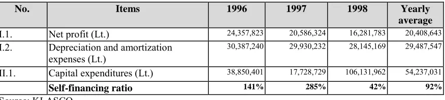
Table 2.4: Self-financing ratio (1996 - 1998)
No. Items 1996 1997 1998 Yearly
average
I.1. Net profit (Lt.) 24,357,823 20,586,324 16,281,783 20,408,643
15
The received self-financing ratio (see Table 2.4) shows that during the analysed period the company was quite sufficient in terms of ability to support its investment needs. Cash inflows generated by the direct operational activities of the enterprise in the years
1996 and 1997 exceeded its strategic cash outflows by 41% and 185% accordingly.
Therefore, theoretically, in these years there was no need for the company to have external financing.
In the year 1998 the cash inflows were 58% less than the strategic outflows. Therefore,
in this year loans are justifiable. However, it is still problematic to say how big the loans had to be. The problem with the cash flow statement is that it doesn’t provide a full information about the other financial sources, which were available for the company at that time. Nevertheless, according to the self-financing ratio the need for the additional financing had to be low because the surplus accumulated in the first two years during the analysed period, had lowered the need from 58% to only 8% (see average figure in Table 2.4).
Now let us look at the fourth part of the cash flow statement.
2.2.4. Cash flow from extraordinary activities
The fourth part of the cash flow statement represents cash flow from extraordinary activities.
eliminating their influence on the enterprise’s investment and financial activities. But it could be that the cash outflows would be shown under the operating activities or the capital expenditure headings. A common practise is to show just the net cash movement as part of operating activities with additional details in the accompanying notes.
In our case there are no amounts disclosed in that part of the cash flow statement therefore we will leave that section as it is.
2.3. Changes in cash balances
Below is the final portion of the cash flow statement (see Table 2.5). This final section sums up the cash flows from the four sub-sections and thus reconciles the cash balances
from one period to the next. The 19,3 millions showed at the bottom-right corner of
Table 2.5 is the amount of cash that exists at the end of our analysed period, and that is
the amount which appears on the company’s 1998 year balance sheet.
Table 2.5: Changes in cash balances (1996 - 1998)
No. Items 1996 1997 1998
Increase (-decrease) of net cash flow -21.883.435 5.343.306 -16.113.618
VI. Cash at the beginning of the period 51.903.913 30.020.478 35.363.784
VII. Cash at the end of the period 30.020.478 35.363.784 19.250.166
Source: KLASCO
As we can see the cash balances of the company have decreased significantly. In a
period from the beginning of 1996 to the end of 1998 they diminished by more than 60%
17
2.4 Conclusions
In this chapter we looked at the amounts of cash held by the company in the period
between the years 1996 and 1998. For this purpose we have examined three cash flow
statements representing that period. We have seen changes in the net cash flow from operating, investment, and financing activities, and changes in cash balances of the company in general. Now, our findings allow us to draw preliminary conclusions about the financial situation and the financial management in KLASCO before privatisation.
The financial situation of the company was quite stable and similar during the first two
analysed years (1996 and 1997), but in 1998 it had changed dramatically. Large amounts
of cash were released, mainly due to the increase in trade payables and the decrease in
prepayments areas. More than 106 million Lt. were invested into long-term assets.
Around 34 million Lt. of loans were taken from the credit institutions.
The big changes in the trade payables and prepayments areas signify a positive attempt by the company to use suppliers’ financial resources to support its business needs. Nevertheless, the efficiency of the financial resource management in KLASCO has to be
questioned and that is mainly due to the need for the loan in the year 1997 and the size
of the loan taken in the year 1998. We will come back to this topic later when we will
look at the sources and uses of the funds in Chapter 6.
19 CHAPTER 3
Working capital analysis
3.1. Introduction
The statement of cash flow gave us an idea where the company’s cash came from and
where the company spent it. But, to consider only the movement of cash over a
period of time does not provide sufficient basis for understanding the financial
changes the business has experienced.
To get a better view of the company’s financial position before privatisation we have
to look at the changes which have occurred within the working capital of the firm.
These changes are important indicators of the business performance. They represent
changes in the amounts of money the enterprise had to work with in the short-term
and give a rough idea about the ability of the company to meet its current obligations
as they fall due. In other words – it gives a crude indication about the liquidity of the
company.
We already mentioned that the working capital is expressed as the difference between
current assets and current liabilities of an enterprise. Therefore, in order to
understand how changes in the working capital had affected the company’s ability to
finance its operations and its liquidity we have to look at and examine the changes in
First, we will start by looking at the current assets and their effect on the working
capital. Next, we will examine the changes in the current liabilities and how they
influenced the working capital of the firm.
3.2. Current Assets
Current assets are one of the major components of the balance sheet. They are the
assets, which can be easily converted into cash within a fairly short time. It is from
current assets that a company funds its day-to-day operations. If there is a shortfall in
the current assets, then the company has to look for other forms of short-term
funding. Such a situation usually results in borrowings from banks, which in return
means interest payments and depreciation of shareholders’ value.
In Lithuania regulations state that the balance sheet should distinguish four main
kinds of current assets (see Appendix 2):
• cash and equivalents
• short-term investments
• accounts receivable
• inventories and prepaid expenses
We will look at each of them and will try to understand how they influenced changes
in the current assets and, consequently, the working capital of the firm during our
analysed period.
21
transaction, precaution and speculation purposes. We know that a stevedoring
business is not the kind of activity were speculations are common. Such a feature is
more related to a shipping sector where big amounts of cash change hands very often
as ships are bought and sold. Therefore, in our case the transactions and the
precautionary motives should, ideally, dictate the appropriate size of the company’s
cash and bank balances. Thus the important aspect of the internal financial
management of the company is to have the right amount of cash available at any
time, because too much money is wasteful; too little is dangerous.
In Chapter 2 we looked at the cash balances of the company before the privatisation.
We will look at them once again in Chapter 4, when we will analyse the liquidity
ratios and in Chapter 7, when we will look at the defensive interval of the company.
From what we have seen so far it is difficult to say how adequate the size of the cash
balances was in the analysed period. However, in terms of the current assets, which
we analyse now, we could conclude that the decline in the cash represents a decline
of the current assets, as well.
Now, let us look at other parts of the current assets.
3.2.2. Short-term investments
Short-term investments are a step below cash and equivalents. These normally come
into play when a company has so much cash on hand that it can afford to tie some of
it up in short-term marketable securities with duration of less than one year. This
money cannot be immediately liquefied without some effort, but it does earn a higher
return than cash by itself. For the financial analysis purposes they are treated as being
As we can see from table 3.1 in the year 1996 the company had invested 8 millions
into short term securities. The cash flow statement reflects that it collected this
money in the year 1997. In the following years there were no more investments.
Table 3.1: Short-term investments (1996-1998)
No. Item 1996 1997 1998
III. Short-term investments (Lt.) 8,000,000 0 0
Source: KLASCO
We could assume that the investment in the year 1996 is an expression of a clear cash
surplus, which the company had at that time. The absence of such investments in the
following years shows that the company had used this money for some purposes,
probably invested into inventory or tangible assets. Therefore, we could say that in
terms of short-term investments, the company’s current assets had declined too.
3.2.3. Accounts receivable
The short-term accounts receivable are used to describe the money that is currently
owed to a company by its debtors. It is expected that the company will receive these
moneys within 12 months. The reason why such debts arise is that the customers
have not paid for the provided services yet, which is not an uncommon situation.
Companies routinely buy goods and services from other companies using credit. In
our case the stevedoring company extends a credit to its customers for the cargo
handling operations and warehousing services. Although it is expected that customers
will pay within a fairly short time there are instances where the company has to
write-off accounts receivable for bad debt accounts, because it has given credit to
23
• trade debtors
• other amounts receivable
Trade debtors are used to account for debts related to operational activities of the
company. Other accounts receivable signify debts which could arise from selling
assets of the enterprise on credit, excess tax amounts to be transferred to the
government budget or other activities, not related to the operations. Let us look at
both categories.
Table 3.2: Changes in accounts receivable (1996-1998)
No. Item 1996 1997 1998
II. Amounts receivable within one year (Lt.) 51.553.044 41.374.807 39.702.931
II.1. Trade debtors (Lt.) 13.624.062 20.999.426 22.381.817
II.2. Other amounts receivable (Lt.) 37.928.982 20.375.381 17.321.114
Source: KLASCO
Table 3.2 shows that the credit extended to the trade partners was continuously
increasing. In the year 1998 it reached more than 22 million Lt. On the other hand
other amounts receivable were constantly decreasing. All together in the period 1996
and 1998 the accounts receivable of the company declined by 23%. It means that the
management of the firm does put in some efforts to secure cash resources of the
company.
The decrease in accounts receivable represent a decrease in the current assets of the
company.
Later, in Chapter 5, we will look at accounts receivable turnover as another way to
3.2.4. Inventories
The least liquid of the company’s current assets is inventory. The inventory account
is used to show stocks of the enterprise. This account is debited when raw materials,
supplies and consumables are purchased and credited after consumption or sale of
supplies and raw materials in form of services.
It is important to distinguish prepayments and contracts in progress from the rest of
inventory, because these are the inventories which have not reached a tangible form
yet. Prepayments are money the company has paid in the current period for goods or
services to be received in a following accounting period. Contracts in progress are
used to account for the value of construction or other contracts in progress.
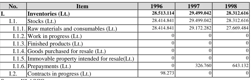
From Table 3.3 we can see that prepayments and contracts in progress have no big
influence on the total amount of the inventories. Therefore, for our future analysis we
will use only the figures representing the total amount of inventories.
Table 3.3: Changes in inventories level (1996-1998)
No. Item 1996 1997 1998
I. Inventories (Lt.) 28.513.114 29.499.042 28.312.616
I.1. Stocks (Lt.) 28.414.841 29.499.042 28.312.616
I.1.1.Raw materials and consumables (Lt.) 28.414.841 29.172.282 27.669.484
I.1.2.Work in progress (Lt.) 0 0 0
I.1.3.Finished products (Lt.) 0 0 0
I.1.4.Goods purchased for resale (Lt.) 0 0 0
I.1.5.Immovable property intended for resale(Lt.) 0 0 0
I.1.6.Prepayments (Lt.) 0 326.760 643.132
I.2. Contracts in progress (Lt.) 98.273 0 0
Source: KLASCO
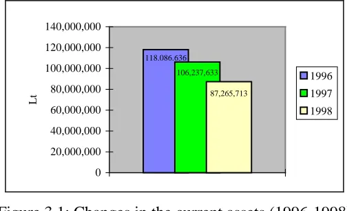
25 3.2.5. Changes in the current assets
We have looked at different components of the current assets. Analysis showed us
that almost all of them had declined. It consequently affected the total amount of the
current assets of the company. From the year 1996 to the year 1998 they diminished
by almost 26% (see Figure 3.1).
118.086.636 106,237,633
87,265,713
0 20,000,000 40,000,000 60,000,000 80,000,000 100,000,000 120,000,000 140,000,000
Lt
1996
1997
1998
Figure 3.1: Changes in the current assets (1996-1998)
Source: KLASCO
Now let us look at the changes which occurred within the current liabilities of the
company.
3.3. Current liabilities
Current liabilities or accounts payable is the money that the company currently owes
to its suppliers, its partners and its employees. Basically, these are the basic costs of
doing business that a company, for whatever reason, has not paid off yet.
The Lithuanian accounting regulations distinguish six main categories of current
liabilities in the balance sheet (see Appendix 2):
•••• current portion of long-term debts
•••• trade creditors payable within one year
•••• prepayments received on contracts in progress
•••• taxes, remuneration and social security costs
•••• other amounts payable within one year and short-term liabilities
Not all of them have affected the position of the company during our analysed period.
No expenses were associated with the current portion of long-term debts; financial
short-term debts; or prepayments received on contracts in progress. Therefore, we
will leave them and will concentrate our attention only on trade creditors,
remuneration and social security costs, and other amounts payable within one year.
We will look at how these three categories have influenced the current liabilities and,
consequently, the working capital of the company.
3.3.1. Trade creditors
The account of trade creditors payable within one year is used to show the short-term
trading debts payable within one year. This account is debited when paying off
trading debts for suppliers’; repurchasing previously issued bills of exchange and
returning customers’ cash guarantees. The account is credited when entering into new
trading debts related to the acquisition of supplies, raw materials and consumables,
issuing bills of exchange for goods acquired as well as receiving cash guarantees
from customers.
Table 3.4 shows that the level of trade creditors has gone up rapidly in the year 1998.
27
Such a radical change in the amounts owed to the creditors could be interpreted in
two ways:
•••• either the company was running out of resources and therefore it went into debt to its suppliers;
•••• or, changes in the company’s financial policy towards a more aggressive use of
suppliers’ financial resources.
The use of the suppliers’ financial resources is considered to be a good financial
management practise because it allows the company to have a credit, usually
interest-free, which can be used to finance its operations.
An increase in the trade creditors in 1998 resulted into huge growth in the total
accounts payable of the company. It means that the current liabilities had increased.
Now, let us look how the other two categories have influenced the total amount of
the current liabilities.
3.3.2. Taxes, remuneration and social security costs
Taxes, remuneration and social security costs used to show the debts related to profit,
VAT, social security taxes, taxes deducted from salaries and other similar
obligations. This account is used to calculate the debt of the enterprise to the
employees as well.
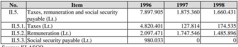
Table 3.5. Changes in the taxes, remuneration and social security level (1996-1998)
No. Item 1996 1997 1998
II.5. Taxes, remuneration and social security payable (Lt.)
7.897.905 1.875.360 1.660.431
Table 3.5 shows that the company has been quite successful in reducing taxes paid to
the Government. In the year 1996 the amount paid to the authorities was close to 5
million Lt. but in the following two years it went dramatically down to just one
hundred twenty seven – one hundred seventy four thousands Lt.. Mainly, such a
decrease was possible due to new regulations, which allowed companies to hide taxes
payable under plans for future investments.
3.3.3. Other amounts payable
Other amounts payable within one year represent short-term liabilities used to
account for debts related to dividends, securities, entitlements and other short-term
payable amounts not accounted in other accounts.
Table 3.6: Changes in the other amounts payable (1996-1998)
No. Item 1996 1997 1998
II.6. Other amounts payable and short-term liabilities (Lt.)
2.376.092 4.026.922 2.058.741
Source: KLASCO
Table 3.6 shows us that other amounts payable remained more or less the same
during our analysed period. There was an increase in the year 1997 but in general it
has not affected the total amount of current liabilities at the end of the period because
in the year 1998 the level of the other amounts payable went down.
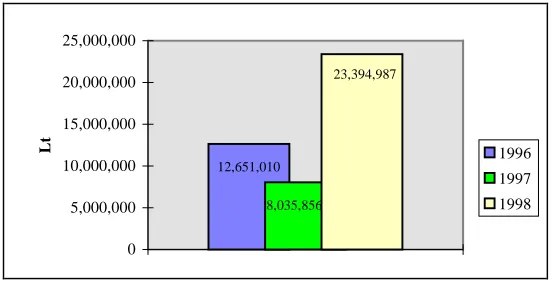
29 12,651,010
8,035,856
23,394,987
0 5,000,000 10,000,000 15,000,000 20,000,000 25,000,000
Lt 1996
1997
1998
Figure 3.2: Changes in the current liabilities (1996-1998)
Source: KLASCO
As we can see a general trend indicates that the current liabilities have increased. It
means that eventually the company was becoming more and more dependent on its
creditors. There has been an especially big increase in the current liabilities in the last
year before the privatisation. They went up by almost 50%.
3.4. Changes in the working capital
Now, after we have looked at the changes that occurred within the current assets and
the current liabilities of the company, we could better understand how these changes
have influenced the working capital of the firm.
As we know, during our analysed period the current assets of the company have
decreased and the current liabilities went up. Automatically it had an effect on the
working capital and liquidity of the company, because, as was mentioned above, it is
expressed as the difference between the current assets and the current liabilities.
From Table 3.7 we can see that the working capital of the company has decreased
Table 3.7: Changes in the working capital of the company (1996-1998)
Item 1996 1997 1998
Current assets (Lt.) 118,086,636 106,237,633 87,265,713
Current liabilities (Lt.) 12,651,010 8,035,856 23,394,987
Working capital (Lt.) 105,435,626 98,201,777 63,870,726
Source: KLASCO
In order to understand how the decrease in working capital has affected the
company’s ability to finance its operations we have to relate it to the sales revenues.
3.4.1. Working capital to sales ratio
The working capital to sales ratio provides an insight into the adequacy and
consistency of the working capital management within the firm. For this measure we
will ignore cash and investments (Vause, 1999, p. 176). Such step will allow us to
see in more precise how much of the company’s financial resources were tied up in
the current assets in order to maintain a constant level of operations. The ratio is
expressed in an equation:
Working capital to sales ratio = Working capital without cash and equivalents x100% Sales revenues
Table 3.8: Working capital to sales revenue ratio (1996-1998)
Item \Year 1996 1997 1998
Current assets without cash and equivalents (Lt.) 80,066,158 70,873,849 68,015,547
Current liabilities (Lt.) 12,651,010 8,035,856 23,394,987
Working capital without cash and equivalents (Lt.) 67,415,148 62,837,993 44,620,560
Sales revenues (Lt.) 182,908,238 179,437,517 163,831,390
Working capital to sales revenue ratio (Lt.) 36.9% 35.0% 27.2%
31
than in the two previous years (see Table 3.8). However, the decrease in the working
capital might also indicate that the company was over-stretching its financial
resources and might be trying to finance too high level of trading with too little
working capital. Such a phenomenon is called overtrading.
3.5. Conclusions
We looked at the changes that occurred within the current assets and the current
liabilities of the company. We have seen how it affected the working capital of the
firm. It was in constant decline.
As the working capital represents a crude measure of liquidity, we could conclude
that during the analysed period the liquidity of the company was declining too. Such
a situation raises a question whether the liquidity of the firm was becoming too low
and because of that it was necessary to sell the company as soon as possible. In order
to answer this question we will examine the company’s liquidity in more detail in
Chapter 4.
The decline in the working capital also indicates a decline in the amounts of money
the enterprise had to work with in the short term. We looked at it in Section 3.4.1 of
this chapter. Our findings allow us to conclude that, in general, a substantial decrease
in amounts of money needed to support the business operations in the year 1998
could be taken as a positive sign of the financial resource management. Nevertheless,
it could also indicate that the company was over-stretching its financial capabilities
or in other words - overtrading.
We will come back to the analysis of the adequacy of the working capital in
CHAPTER 4
Changes in the liquidity of the company
4.1. Introduction
In Chapter 2 and Chapter 3 we have looked at changes in the cash position and the
working capital of the Klaipėda Stevedoring Company before privatisation. The analysis of changes has shown a decline in the amounts of money that the enterprise had to work with. We mentioned that this decline could be taken as a sign representing a decrease in the company’s ability to pay its short-term obligations, or in other words - liquidity.
In this chapter we will look at the liquidity in more detail. For this purpose we will relate the company’s current assets and current liabilities into liquidity ratios.
The first step will be to relate the total current assets to the total current liabilities of the company in what is commonly termed as the current ratio.
The next step – to eliminate the inventories from the current assets and relate the rest to the current liabilities in the liquid or quick ratio.
33
Such an approach to the analysis of the company’s ability to pay its short-term obligations is necessary due to the different liquidity levels of the current assets’ components. As was pointed out in Chapter 3, the most liquid assets of the company
are money and equivalents, they are followed by the short-term investments, then the accounts receivable, and finally the inventories. Thus, the more liquid the company is the higher proportion of its current assets will be in cash or near-cash items.
Now, let us look at the situation of KLASCO.
4.2. Current ratio
The current ratio measures the ability of a business to meet its short-term liabilities in general. It compares the total amount of current assets to the total amount of current liabilities and is expressed by the formula:
Current ratio = current assets/ current liabilities
If this ratio is less than 1:1 it indicates that the business will probably have difficulty meeting its debts in the short term.
A ratio between 1:1 and 2:1 indicates that the business should be able to meet its short-term debts but may not have available working capital to do things such as increase stocks or to cover any trading losses.
A ratio above 2 indicates that the company should be able to pay its debts and have available working capital for other uses.
Table 4.1: Changes in the current ratio (1996 - 1998)
Item \Years 1996 1997 1998
Current assets (Lt.) 118.086.636 106.237.633 87.265.713 Current liabilities (Lt.) 12.651.010 8.035.856 23.394.987
Current ratio 9,3 13,2 3,7
Source: KLASCO
As we can see from Table 4.1 the current ratio of KLASCO was very high during the analysed period. In the year 1996 it was at a level of 9,3; in 1997 at 13,2. In 1998 the ratio had dropped to 3,7, but still, the company had almost four times the amount of total current assets as it had liabilities. It means that in the year 1998 if the company would have had to repay its short-term obligations in full it would have had to liquidate its current assets only at about 25% of their book value.
Although the analysed ratio is obviously very high it fails to provide a clear picture about the liquidity of the company. As we already mentioned, to look at the total amounts of the current assets in the balance sheet is not sufficient, because of different liquidity levels of the current assets’ components. Therefore, the next step is to eliminate the least liquid component of the current assets and to see how the situation would change. The new ratio is called liquid or quick ratio.
4.3. Quick ratio
35
Quick ratio = (current assets - inventory)/ current liabilities
If the value of this ratio is much less than 1:1 it indicates that the firm might have a liquidity problem, as it may have insufficient assets to meet all its immediate liabilities.
A quick ratio of 1:1 and above indicates that a company should have enough liquid resources to be able to meet all of its current obligations almost immediately.
Now, let us consider the situation with our analysed company.
First of all, we eliminate the inventory, which as we can see from Table 4.2 was a continuously increasing portion of the current assets, although the amount was relatively stable.
Table 4.2: Changes in the inventory holding level (1996 - 1998)
Item \Year 1996 1997 1998
Inventory (Lt.) 28,513,114 29,499,042 28,312,616
Current assets (Lt.) 118,086,636 106,237,633 87,265,713
Inventory holding (%) 24% 28% 32%
Source: KLASCO
Next, we compare the resulting figure of the current assets to the total current liabilities (see Table 4.3).
Table 4.3: Changes in the quick ratio (1996 - 1998)
Item \Years 1996 1997 1998
Current assets without the inventory (Lt.) 89.573.522 76.738.591 58.953.097 Current liabilities (Lt.) 12.651.010 8.035.856 23.394.987
Quick ratio 7,1 9,5 2,5
Once again the liquidity ratio is quite high. Although in the year 1998 it was at the lowest level (2,5), the company still had more than two times in liquid assets than it had current liabilities. It shows that even when inventory was excluded, the company had enough financial resources to pay its debts.
A more strict approach to the liquidity, apart from excluding the inventories, is to eliminate trade receivables from the current assets and compare what is called the most liquid resources of the company - cash balances and short term investments to the total current liabilities.
4.4. Cash and short term investments to the total current liabilities ratio
Although both of the analysed ratios show that the liquidity of the company was high, and in many cases this fact would be acceptable as sufficient evidence of the company’s ability to meet its short term obligations, for the purpose of the financial analysis we took one more step ahead. Apart from inventories we eliminated the trade receivables from the current assets and compared what is called the most liquid resources of the company - cash balances and short term investments to the total current liabilities (see Figure 4.1).
37
Table 4.4: Increase in trade debtors (1996 - 1998)
Item \Year 1996 1997 1998
Trade debtors (Lt.) 13.624.062 20.999.426 22.381.817 Source: KLASCO
If the level of bad debts in the accounts receivable indeed was high, the high liquidity ratios of the company would be justifiable. However, the comparison of cash balances and short-term investments to the total current liabilities (see Figure 4.1) reveals that even if the inventories and the accounts receivable would not be available, the company still had enough financial resources to cover its short-term obligations.
23,394,987 19,250,166 35,363,784 38,020,478
12,651,010
8,035,856 0 5,000,000 10,000,000 15,000,000 20,000,000 25,000,000 30,000,000 35,000,000 40,000,000
1996 1997 1998
Years
Lt
Cash and short term investments Current liabilities
Figure 4.1: Comparison of cash balances to current liabilities (1996 - 1998)
Source: KLASCO
The results shown in Figure 4.1 confirm that the company was highly liquid during the entire analysed period and was able to repay its current liabilities almost immediately.
4.5. Conclusions
In order to get a thorough insight into the company’s ability to meet short-term obligations, we eliminated one by one the least liquid assets from the current assets and compared the rest to the total short-term liabilities.
Now, we can answer the question raised at the end of Chapter 3, whether the
liquidity of the firm was becoming too low.
The result of the analysis allows us to draw a conclusion that the company was too liquid during the analysed period. It was able to repay its short-term debts immediately just from its cash balances. Such a situation shouldn’t be considered as healthy. Therefore, a sharp decrease in the liquidity ratios during the year 1998 (see Figure 4.2) should be considered as a positive change in the company’s financial position.
Figure 4.2: Evolution of the current and quick ratio (1996 - 1998)
Source: KLASCO
3.7
13.2 9.3
2.5
7.1
9.5
0.0 5.0
10.0
15.0
1996 1997 1998
Years
39
CHAPTER 5
The cash cycle
5.1. Introduction
We have looked at the cash balances and the working capital of the company in
Chapters 2 and 3. We have discussed the relationship between the current assets and
current liabilities in Chapter 4. We have seen that the situation has changed from
year to year, and in fact, it changed not only from year to year but also from day to
day as the company was conducting its business.
The cash was turning around in the business on a continuing basis. It was used to
purchase inventory, to pay the invoices to suppliers, and when service was provided,
cash was collected from the customers (see Figure 5.1).
Figure 5.1: The cash cycle
Source: KLASCO
Debtors Creditors
On each turn of the cycle the company was making a profit. The services were sold,
hopefully, for more than the cost of their production, resulting in more cash available
to expand the business.
One thing, which we didn’t consider in detail in our prior analysis, was that most
transactions were done on credit and it means the time element was involved. The
company as a buyer almost always had a short period of time before it paid its
suppliers for goods and services. The company as a seller almost always had to wait
before the customers would make their payments.
Therefore, in this chapter we will look at the length of time that it took for the
company to convert cash outflows into cash inflows. We will do this by analysing
how the cash was flowing around the business in the cash or working capital cycle.
For the ease of the investigation we will divide the cycle into three sub-cycles:
• inventory cycle
• accounts receivable cycle
• accounts payable cycle
The analysis, should allow us to determine the amount of capital the company needed
to operate, and show how efficient it was in using credit and accounts receivable
collection policies to support the business.
We will start the analysis by looking at the average daily sales and average daily
costs, which will be used later as key dominators in calculating the inventory,
41 5.2. Average daily sales and costs
The average daily sales and costs (hereinafter referred as ADS and ADC) are useful
indicators of the company’s short-term cash flows and financial position. They give a
broad idea of how much more the company has received than it spent. The indicators
are calculated by dividing sales and cost of sales that reflected in the year end
financial statements of the company by the number of days in a year.
For the calculations some accounting books recommend to use a number of 240 days
(working days in the year), some - 360 days (30 days per month x 12 months), others
- 365 as a dominator (Vause, 1999, p.177). In our case we have used 365 days a year.
Now, let us look at the figures (see Table 5.1).
Table 5.1: Average daily sales and costs (1996 - 1998)
Item \Years 1996 1997 1998
Total sales (Lt.) 182.908.238 179.437.517 163.831.390
Total costs (Lt.) 157.395.758 156.497.778 149.619.941
ADS (Lt.) 501.118 491.610 448.853
ADC (Lt.) 431.221 428.761 409.918
Source: KLASCO
As we can see in the year 1996 the ADS was 501.118 Lt. and the ADC - 431.221 Lt.
In the following years the figures have slightly declined, but not very much (see
Figure 5.2.). It indicates that during the analysed three-year period the company had
0 100.000 200.000 300.000 400.000 500.000 600.000
1996 1997 1998
Years
Lt
ADS
ADC
Figure 5.2: Changes in the average daily sales and costs (1996 - 1998)
Source: KLASCO
Combined with the other information from the balance sheet, the ADS and ADC will
now help us to understand the way the cash was flowing around the business.
Let us start from looking at the inventory cycle.
5.3. Inventory cycle
The inventory cycle measures the length of time it took for the business to convert
inventory into cost of sales. It represents the number of days the cash was tied up in
inventory.
The way to calculate the length of time it took to convert inventory into cost of sales
is by dividing the year-end balance figure for the inventory by the ADC. The ADC is
used because inventory is valued at the net realisable value, so there is no profit
43
In general, the lower the number of days received from the equation, the better it is
for the company. It means less financial resources were tied up in a
non-profit-generating item. Besides, the inventory is expensive to keep. Bigger stocks would
require large warehouses, more people employed and then would be more chances
for the stock to become obsolete, damaged or even stolen. However, a too small
number of days received from the equation might indicate that the company did not
have a sufficient inventory level, and it could mean problems in satisfying needs of
customers.
Now, let us consider the situation with KLASCO.
Table 5.2. Number of days the inventory was held (1996 - 1998).
Item \Year 1996 1997 1998
Inventory (Lt.) 28.513.114 29.499.042 28.312.616
ADC (Lt.) 431.221 428.761 409.918
Inventory held (d.) 66 69 69
Source: KLASCO
As we can see, during the analysed period, on average, the company was turning over
the value of its entire stock every 66 - 69 days. The figures are quite stable. It shows
that the company had more or less stable demand and consumption of the inventory.
Nevertheless, an increase in a number of days’ the inventory was held in 1997 and
1998, shows that in comparison with 1996 the situation got worse. Although the
difference of three days might look not very significant, it represents a need for
additional assets equal to almost 1,3 million Lt. in the year 1997 and a little bit less in
the year 1998.
If it would prove to be possible to reduce the level of inventory from 69 days back to
the previous level of 66 days, not only would there be no need for the additional
assets but the cash cycle would speed up, the profit margin would be achieved three
An alternative way to look at the efficiency of inventory levels is to calculate the
inventory turnover for the year. In order to do that we will divide the annual cost of
sales by year-end inventory:
Inventory turnover = Annual total costs/ Inventory.
For this ratio, the higher the resulting figure the more effective is a company’s
management of inventory. However, too high a result, again, might indicate an
insufficient level of inventory.
Table 5.3. Inventory turnover ratio (1996 -1998)
Item \Year 1996 1997 1998
Total costs (Lt.) 157.395.758 156.497.778 149.619.941
Inventory (Lt.) 28.513.114 29.499.042 28.312.616
Inventory turnover ratio 6 5 5
Source: KLASCO
From Table 5.3 we see that the company’s inventory turnover in 1996 was six times
per year, in 1997 and 1998 – five times. Although the speed of the turnover has
slowed down a little bit, it still seems to be quite a good result for a stevedoring
company, bearing in mind the amounts of money involved.
In order to get an even deeper insight into KLASCO inventory management we will
exclude the prepayments from the inventory and will break down the stock of the
company into product groups. The key idea of such a move is to distinguish and
pinpoint the areas, which might be considered problematic in terms of cash flows,
45
Table 5.4. Number of days the stock was held (1996 - 1998)
Item \Year 1996 1997 1998
Raw materials (Lt.) 11.845.334 12.314.569 14.873.379
Package (Lt.) 16.052 21.893 25.938
Fuel and oil products (Lt.) 606.878 601.163 456.051
Building materials (Lt.) 5.000.765 4.463.063 0
Spare parts (Lt.) 10.860.945 11.656.535 12.314.113
ADC (Lt.) 431.221 428.761 409.918
Raw materials (d.) 27 29 36
Package (d.) 0,04 0,05 0,06
Fuel and oil products (d.) 1 1 1
Building materials (d.) 12 10 0
Spare parts (d.) 25 27 30
Source: KLASCO
The analysis reveals that the company has no big need for package, and has no
problems with the fuel and oil products supply. The stock was kept just to satisfy
daily operational needs.
The need for raw materials was increasing each year but at the same time it was
decreasing for building materials. It is interesting to notice that the amount of raw
materials has increased almost exactly by the amount that building materials have
decreased. It is difficult to say if there is any correlation between these two elements.
It might be that in the year 1998 the building materials were accounted for raw
materials. Therefore, it is hard to evaluate the increase in the level of raw materials.
Nevertheless, proactive management and supply chain revision, probably, would
prove it possible to reduce the raw materials to a level more beneficial for the
company.
The stock of spare parts had also increased. It went from 25 to 30 days during the
analysed period. This increase might be a signal that the equipment of the company
was becoming obsolete, but again, in order to be sure, a detailed analysis of the
5.4. Accounts receivable cycle
This cycle measures the length of time it took for the business to convert a sale of
services into cash. Such knowledge is important because profits come only from paid
sales.
The cycle is calculated by dividing the total year-end figure of the trade debtors on
the balance sheet by the average daily sales (ADS):
Days’ credit given = Trade debtors/ ADS.
The longer the debtor period, the greater the risk that debts will turn out to be bad
debts, or will take considerable effort and cost to be collected. If the debtor period is
lower the company is getting its cash back quicker and has the possibility to put it
immediately in use. This is a crucial edge; to have cash returned earlier because the
money that is not tied up in accounts receivable is a financial resource that can be
used to expand the business.
Now let us look at the situation with KLASCO.
Table 5.5. Level of credit offered to customers (1996 - 1999)
Item \Years 1996 1997 1998
Trade debtors (Lt.) 13.624.062 20.999.426 22.381.817
ADS (Lt.) 501.118 491.610 448.853
Credit period offered to customers (d.) 27 43 50