Confidence sets for change-point problems
in nonparametric regression
Dissertation
zur Erlangung des Doktorgrades
der Mathematisch-Naturwissenschaftlichen Fakultäten vorgelegt dem
Fachbereich Mathematik und Informatik der Philipps-Universität Marburg
von
M. Sc. Viktor Bengs
geboren in Kaptschagajder Philipps-Universität Marburg (Hochschulkennziffer 1180) als Dissertation angenommen am 18. September 2018
Erstgutachter: Prof. Dr. Hajo Holzmann Zweitgutachter: Prof. Dr. Natalie Neumeyer
Tag der Einreichung: 12. Juli 2018 Tag der Disputation: 27. September 2018
Acknowledgments
First and foremost, I want to thank my supervisor, Hajo Holzmann, for his superb support at any time, for the enlightening discussions we have had and for his honest criticism which improved this thesis as well as broadened my scientific knowledge significantly. Moreover, I thank Prof. Dr. Natalie Neumeyer for making the second assessment of this thesis. I thank my fellow working group members and my colleagues for the throughout nice working atmosphere, the interesting talks during lunchtime, the funny board game parties and especially for enduring my uncountable many bad jokes. Special thanks to Jasmin Hill and Heiko Werner for reading parts of this thesis and giving valuable comments as well as helpful corrections. Great thanks to my family and my friends for always bolstering me up. Thank you, Jasmin, for being there for me at any time. I gratefully acknowledge financial support from the DFG, grant Ho 3260/5-1.
Contents
Zusammenfassung 1
Introduction 5
Notation 9
1. Nonparametric regression and change-point problems 11
1.1. Nonparametric regression and minimax estimation theory . . . 11
1.2. Change-point analysis under nonparametric regression . . . 14
1.2.1. Estimation of change-point-locations in univariate frameworks . . . 15
1.2.2. Estimation of change-point-locations in multivariate frameworks . . . 19
1.3. Uniform M- and Z-estimation theory . . . 21
1.3.1. Uniformity over the function class . . . 21
1.3.2. Uniformity over the covariate space . . . 22
1.3.3. Distinct rates of convergence . . . 24
1.4. Confidence sets . . . 24
1.5. Confidence sets in nonparametric regression with change-points . . . 30
2. Asymptotic confidence sets for the jump curve in bivariate regression problems 33 2.1. Model and estimate . . . 33
2.2. Asymptotic theory . . . 34
2.3. Simulations . . . 37
2.4. Outline of proofs . . . 43
2.4.1. Uniform consistency . . . 44
2.4.2. Rate of convergence: proof of Theorem 2.1 . . . 47
2.4.3. Asymptotic normality: proof of Theorem 2.2 . . . 49
2.4.4. Uniform confidence bands: proof of Theorem 2.3 . . . 50
2.5. Discussion . . . 53
2.6. Detailed proofs . . . 54
2.6.1. Order of the asymptotic bias: proof of Lemma 2.7 . . . 54
2.6.2. Convergence of the Hessian matrix: proofs of Lemma 2.8 and Lemma 2.11 58 2.6.3. Asymptotic normality of the score: proof of Lemma 2.10 . . . 64
2.6.4. Gaussian approximation: proofs of Lemmas 2.13, 2.15 and of Proposition 2.9 66 2.6.5. Rate of convergence of the Hessian matrix: proof of Lemma 2.12 . . . 67
2.6.6. Quantile approximation: proofs of Lemma 2.14 and Lemma 2.16 . . . 68
3. Adaptive confidence intervals for kink estimation 71 3.1. The zero-crossing-time-technique . . . 71
3.1.1. Model and assumptions . . . 71
3.2. Asymptotic confidence sets . . . 75
3.2.1. Asymptotic normality of the estimates . . . 75
3.2.2. Adaptive confidence sets . . . 76
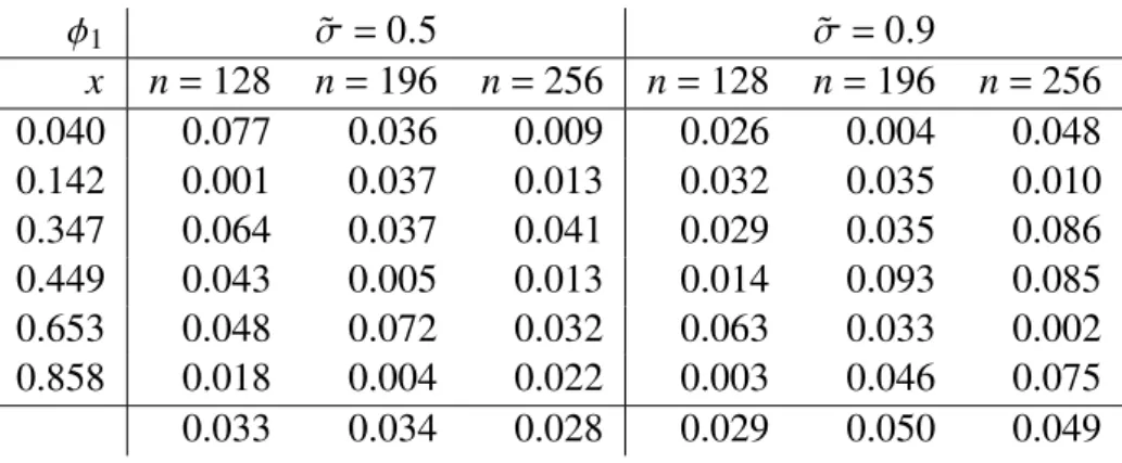
3.3. Finite sample simulations . . . 78
3.4. Discussion . . . 88
3.5. Proofs . . . 89
3.5.1. Properties of the probe functional . . . 89
3.5.2. Uniform consistency of the first stage of the zero-crossing-time-technique . 94 3.5.3. Exponential concentration inequality . . . 96
3.5.4. Rates of convergence: outlines of the proofs of Theorems 3.3 and 3.4 . . . 97
3.5.5. Asymptotic normality: outline of the proof of Theorem 3.5 . . . 99
3.5.6. Proofs of auxiliary results in Section 3.5.4 and 3.5.5 . . . 100
3.5.7. Adaptive confidence sets: proof of Theorem 3.7 . . . 104
3.6. Kernel construction . . . 112
4. Lower bounds for change-point-locations in nonparametric regression 119 4.1. General theorem for deriving minimax lower bounds . . . 119
4.2. Bivariate boundary fragment model with fixed design . . . 120
4.3. Kink-location with fixed design . . . 122
A. Gaussian and sub-Gaussian processes 127 A.1. Properties of Gaussian processes . . . 127
A.1.1. Proof of Lemma A.1 . . . 129
A.1.2. Proof of Lemma A.3 . . . 133
A.2. Properties of sub-Gaussian processes . . . 136
B. Asymptotics of components of the contrast function and their derivatives 139 B.1. Bivariate design . . . 139
B.2. Univariate design . . . 143
C. Extended probability theory 145
Zusammenfassung
Nichtparametrische Regression hat über die letzten Jahre in der Statistik und anderen Bereichen große Aufmerksamkeit genossen. Die Anwendungsbereiche sind vielfältig und spielen für die Modellie-rung von Zusammenhängen zwischen verschiedenen Merkmalen eine große Rolle. Insbesondere wird oftmals mittels der nichtparametrischen Regression ein digitales Bild modelliert, indem die Bildintensitätsfunktion als Regressionsfunktion verwendet wird und die Pixel als erklärende Varia-blen. Dadurch besteht ein starker Zusammenhang zu dem Bereich der Bildverarbeitung.
Eine weiterer wichtiger Teilbereich von Regressionsproblemen sind solche, bei denen Irregularitäten in der Regressionsfunktion vorhanden sind, sodass die klassischen Glattheitsannahmen über den gesamten Definitionsbereich nicht gelten können. Solche Irregularitäten werden in eindimensiona-len Regressionsproblemen change-points genannt und change-curves im multivariaten Fall. Sprünge oder Knicke in der Regressionsfunktion sind Beispiele für change-points, wohingegen change-curves in der Regel Unstetigkeitskurven entsprechen. Unstetigkeitskurven einer Bildintensitätsfunktion für zweidimensionale Bilder werden Kanten genannt und stellen ein allgegenwärtiges Objekt in diesem Bereich dar.
Klassische Glättungsverfahren wie zum Beispiel Kernregressions-, lokale Polynom- oder Wavelet-projektionsschätzer sind für Regressionsprobleme mit change-points beziehungsweise change-curves nicht mehr optimal. Dies liegt daran, dass diese Methoden bei der Entfernung des Rauschens der Beobachtungen die change-points als solches Rauschen missinterpretieren würden und diese fälsch-licherweise mitglätten. Dies würde in schlechten Schätzwerten für die Regressionsfunktion in der Nähe der change-points resultieren.
Um die Nachteile der klassischen Glättungsverfahren zu kompensieren, wurden in der Literatur al-ternative Methoden entwickelt. Insbesondere spielen für diese Methoden die explizite Schätzung der Stellen, der Ausprägung und der Anzahl der change-points eine zentrale Rolle, da diese wichtige Merkmale der Regressionsfunktion darstellen, die für eine adäquate Schätzung der Regressionsfunk-tion berücksichtigt werden müssen. Diese Arbeit befasst sich primär mit der Schätzung der Stellen, an denen change-points auftreten, sowie der damit verbundenen Unsicherheit der Schätzung, welche durch Konfidenzmengen erfasst wird. Entsprechend beschränkt sich die Diskussion der Literatur auf diese Themen.
Der mit Abstand meist studierte Typ von change-points ist eine Sprungstelle in der Funktion von Interesse. Eine weitverbreitete Methode um Sprungstellen in eindimensionalen Regressionsproble-men zu schätzen bzw. auf Sprungstellen zu testen, ist die geglättete Differenzenmethode, welche in Qiu und Li (1991), Müller (1992) bzw. Wu und Chu (1993) eingeführt wurde. Die Grundidee dabei ist, dass die absolute Differenz zwischen einem linksseitigen Kernschätzer und einem rechtsseitigen Kernschätzer in Bereichen, in denen die Funktion glatt ist, klein ist, jedoch in der Nähe von Sprün-gen große Werte annimmt. Entsprechend ist die Stelle, an dem diese Differenz maximal wird, ein sinnvoller Schätzer für die Sprungstelle.
Dieser Ansatz ist für den eindimensionalen Fall gut geeignet, jedoch ist es nicht ohne weiteres möglich, dieses Konzept auf den mehrdimensionalen Fall zu erweitern. Dies liegt daran, dass im
gegen es im eindimensionalen Fall nur zwei Richtungen auf der reellen Zahlengerade gibt. Um dieses Problem anzugehen, haben Qiu (1997) bzw. Müller und Song (1994) die rotierende geglät-tete Differenzenmethode entwickelt, welche es erlaubt, die Differenz der einseitigen Kerne in eine angemessene Richtung zu rotieren. Dadurch kann die Sprungkurve adäquat geschätzt werden, so-dass eine sinnvolle Rekonstruktion der nicht-glatten Regressionsfunktion unter Berücksichtigung der geschätzten Sprungkurven möglich ist.
Abgesehen von der Rekonstruktion bzw. der Schätzung eines Objektes von Interesse ermöglicht sta-tistische Modellierung die Konstruktion von Konfidenzmengen, welche das Objekt mit einer großen Wahrscheinlichkeit enthalten. Konfidenzmengen sind mittlerweile für verschiedene Probleme der nichtparametrischen Statistik gut erforscht, wie z.B. für nichtparametrische Dichteschätzung (Bickel und Rosenblatt (1973), Giné und Nickl (2010), Chernozhukov et al. (2014)), für glatte Regressi-onsfunktionen (Eubank und Speckman (1993), Neumann und Polzehl (1998), Proksch (2016)), und für inverse Probleme, sowie dem Messfehler-Modell (Bissantz und Holzmann (2008), Birke et al. (2010), Proksch et al. (2015), Delaigle et al. (2015)). Konfidenzbereiche für geometrische Merkmale wie Dichtelevelmengen (Mammen und Polonik (2013)) oder Moduskurven von Dichten (Qiao und Polonik (2016)) wurden ebenfalls bereits studiert. Konfidenzintervalle für Sprungstellen in eindi-mensionalen Regressionsproblemen wurden von Loader (1996), Gijbels et al. (2004), sowie Seijo und Sen (2011) konstruiert.
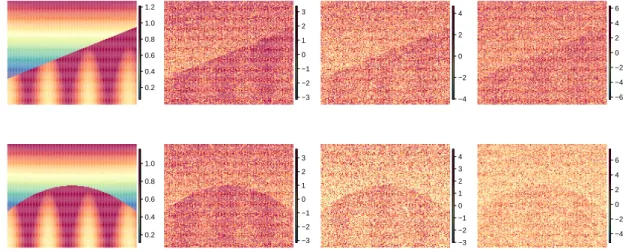
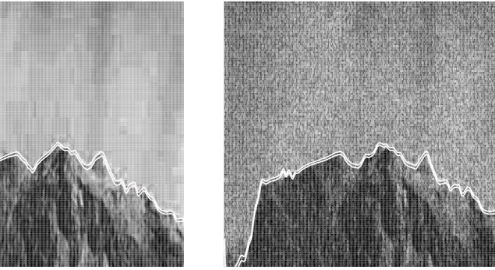
Allerdings gibt es bislang keine Methoden, um Konfidenzbereiche für Sprungkurven in bivariaten bzw. multivariaten Regressionsproblemen zu konstruieren. Um diese Lücke zu schließen, werden in Kapitel 2 gleichmäßige und punktweise asymptotische Konfidenzbänder für eine einzelne Sprung-kurve in einer ansonsten glatten RegressionsSprung-kurve konstruiert. Der Ausgangspunkt dafür ist die rotierende geglättete Differenzenmethode, so dass ein Bezug zu Qiu (2002) besteht, jedoch wird anstelle einer Schwellwertbildung eine Linearisierung einer lokalisierten Version des Kontrastes verwendet, um eine leichtere Anwendung der Techniken aus der M-Schätztheorie zu ermöglichen. Die Konstruktion der gleichmäßigen Konfidenzbänder beruht auf einer Gaußschen Approximation des Score-Prozesses und einer Anti-Konzentrationsungleichung für das Supremum von Gaußschen Prozessen ähnlich wie in Chernozhukov et al. (2014). Für die punktweisen Konfidenzbänder wird asymptotische Normalität der Schätzer verifiziert. Um die Anwendbarkeit der Ergebnisse auf endliche Datenmengen zu illustrieren, wird sowohl eine Simulationsstudie für künstliche Daten durchgeführt, als auch eine Anwendung der Methode auf ein digitales verrauschtes Bild.
Neben Sprungstellen in der Regressionsfunktion selbst gibt es weitere Irregularitäten, die in der sonst glatten Regressionsfunktion auftreten können. Ein weiterer relevanter Typ von Irregularitäten ist ein Sprung in einer der Ableitungen der Regressionsfunktion. Solch ein Punkt hat teilweise auch einen starken Einfluss auf die Form der Regressionsfunktion, da zum Beispiel eine Unstetigkeit in der ersten Ableitung zu einer abrupten Änderung der Steigung der Regressionsfunktion führt, oder eine Unstetigkeit in der zweiten Ableitung in einer plötzlichen Änderung der Krümmung resultiert. Wir nennen Sprünge in derγ-ten Ableitungγ-Knicke oder Knicke der Ordnungγ.
Die Schätzung vonγ-Knicken war Gegenstand der Arbeiten von Müller (1992), Eubank und Speck-man (1994), Wang (1995), Goldenshluger et al. (2006), Goldenshluger et al. (2008a), Cheng und Raimondo (2008), Wishart (2009), Wishart und Kulik (2010) als auch Mallik et al. (2013). Jedoch hat nur Mallik et al. (2013) explizit Konfidenzintervalle für die Stelle eines Knickes höherer Ordnung konstruiert. Die Annahmen an die Glattheit der Regressionsfunktion außerhalb des Knickes sind schwächer als in der Literatur zuvor, allerdings werden einschränkende Annahmen an die Form der Regressionsfunktion gemacht, welche die Anwendbarkeit ihrer Methode limitiert.
Eine effiziente Technik zur Schätzung der Knick-Stelle ist die sogenannte zero-crossing-time-technique, welche die Nullstelle einer geglätteten zweiten Ableitung der Funktion von Interesse als Schätzer benutzt. Die Grundidee ist, dass falls die Funktion von Interesse einen Sprung inθ
auf-weist, so hat eine geeignete geglättete Version dieser Funktion eine große Steigung in der Nähe von θ.Entsprechend hat die erste Ableitung dieser geglätteten Version ein lokales Maximum in der Nähe vonθund die zweite Ableitung dort eine Nullstelle. Die Methode besteht dann aus zwei Phasen: In der ersten Phase wird ein Intervall bestimmt, welches den Knick mit einer hohen Wahrscheinlichkeit enthält. In der zweiten Phase wird der Knick durch eine Nullstelle einer empirischen Version der geglätteten zweiten Ableitung innerhalb des Intervalls geschätzt. Goldenshluger et al. (2006) haben diese Methode verwendet, um die einzelne Sprungstelle in einem indirekten Modell in weißem Rau-schen zu schätzen. Zusätzlich haben sie die Minimax-Optimalität dieser Methode verifiziert, falls die Signalfunktion mindestens Lipschitz-glatt außerhalb der Sprungstelle ist. Um diese Methode auch für ein direktes Problem anwenden zu können, haben Cheng und Raimondo (2008) explizite Kerne für die Glättung der zweiten Ableitung konstruiert, um auf Knicke in der Regressionsfunktion zu testen. Wishart (2009) bzw. Wishart und Kulik (2010) verwendeten dann letztere Modifikation um Knicke zu schätzen, falls das Design oder die Fehler im Regressionsproblem Abhängigkeitsstrukturen auf-weisen. Zwar wurde die Optimalität der Schätzmethode in den gerade genannten Papieren rigoros studiert, jedoch wurden asymptotische Verteilungseigenschaften gänzlich außer Acht gelassen. Dies liegt an der verwendeten Charakterisierung des Schätzers als M-Schätzer, anstatt die natürlich ge-gebene Charakterisierung als Z-Schätzer zu nutzen, so dass Konvergenzraten als M-Schätzer leicht hergeleitet werden können, aber asymptotische Verteilungsergebnisse eher schwer nachweisbar sind. In Kapitel 3 wird die Charakterisierung als Z-Schätzer verwendet, um die asymptotische Norma-lität des Schätzers herzuleiten und somit Konfidenzmengen zu konstruieren. Basierend auf der asymptotischen Normalität und einer Lepski-Wahl des Tuningparameters der zero-crossing-time-technique werden für einen einzelnenγ-Knick adaptive Konfidenzintervalle konstruiert, die sich an die Hölder-Glattheit der Regressionsfunktion außerhalb des Knickes anpassen. Eine Simulationsstu-die für künstliche Daten und einige Anwendungen auf reale Daten unterstreichen Simulationsstu-die Nützlichkeit der zuvor hergeleiteten Ergebnisse.
Diese Arbeit ist wie folgt strukturiert. Das erste Kapitel gibt eine prägnante Einführung in die nötigen theoretischen Konzepte für diese Arbeit. Zudem wird der aktuelle Forschungsstand in der Litera-tur bezüglich der Schätzmethoden und der Konstruktion von Konfidenzmengen für change-points diskutiert. Kapitel 2 konstruiert gleichmäßige und punktweise Konfidenzbänder für eine einzelne Sprungkurve in einem bivariaten Regressionsproblem mittels M-Schätzmethoden und Gaußscher Approximation. Die Resultate basieren größtenteils auf Bengs et al. (2018). Adaptive Konfidenzin-tervalle für einen einzelnen Knick höherer Ordnung werden in Kapitel 3 behandelt, welches auf Bengs und Holzmann (2018) beruht. Kapitel 4 widmet sich der Herleitung der Minimax-Konvergenzraten für die Modelle in den beiden Kapiteln zuvor, um deren Optimalität zu zeigen. Die optimale Konver-genzrate für das Modell in Kapitel 2 ist bereits bekannt, wohingegen die für das Modell in Kapitel 3 neu ist. Schließlich werden im Anhang verschiedene Hilfsresultate bereitgestellt, welche von unab-hängigem Interesse sein können, da diese zum einen bequeme Hilfsresultate für nichtparametrische Regressionsprobleme mit deterministischem Design beinhalten und zum anderen Ergebnisse der klassischen Wahrscheinlichkeitstheorie auf ein Szenario, in dem gleichmäßige Ergebnisse von Inter-esse sind, erweitern.
Introduction
Nonparametric regression has been a topic of major interest over the last years in statistics and other fields. Its application is manifold and plays nowadays an important role for modeling relationships between different features as well as for denoising. In particular, nonparametric regression is often used for modeling an image by interpreting the regression function as the corresponding intensity function of the image and the pixels as the explaining variables. Consequently, there is a strong relationship to the realm of image processing.
An important subdomain of regression problems are frameworks where regression functions with irregularities emerge, such that global smoothness assumptions (in some specific sense) as required in the classical nonparametric regression cannot hold over the whole domain space. Such irregular-ities are called change-points in univariate settings or change-curves in the multivariate extension. Change-points can be for instance jumps or kinks of the regression function, while change-curves usually correspond to discontinuity curves. In two-dimensional image functions, a discontinuity curve of the intensity function of the image is called an edge and is an omnipresent object in this area.
For regression problems with change-points or change-curves the classical smoothing procedures such as kernel-smoothing, local-polynomial or wavelet projection to name a few, are often no longer optimal in the presence of such irregularities. In order to denoise the observations the change-point-locations would be misconceived as noise and consequently be smoothed out at these change-point-locations. The resulting estimators of the regression function would not give a good fit near these change-point-locations.
Alternative procedures have been proposed to circumvent the drawbacks of classical smoothing procedures in a nonparametric regression framework with change-points. In particular, the explicit estimation of the location, the magnitude as well as the number of such change-points play a major role in this realm, as these are specific characteristics of the regression function, which need to be incorporated in order to guarantee a suitable estimation of the non-smooth regression function. The main focus of this thesis is on estimation of change-point-locations and the corresponding un-certainty of this estimation problem expressed through confidence sets, so that discussion of the literature concentrates mainly on this particular issue.
The most studied type of change-point is a jump-discontinuity of a function of interest. One popular method to detect or to estimate jump-point-locations in univariate frameworks is the so called smoothed difference approach which was introduced in Qiu and Li (1991), Müller (1992) resp. Wu and Chu (1993). The basic idea is that the absolute difference of a left-sided kernel estimator and right-sided kernel estimator should be nearly zero at points where the function is smooth, but should be large near a jump-point. Consequently, a sensible estimator for the jump-point-location is given by the point maximizing this difference.
Although this procedure works well in the one-dimensional case, it is not straightforward to extend this method to the bivariate case. This is due to the uncountable infinite many directions around a jump-location-curve in the bivariate setting, while in a univariate setting there are only two directions around the jump-point on the real line. To this end, Qiu (1997) or Müller and Song (1994) proposed
estimators in an appropriate direction. This extension allows a proper estimation of the jump-location-curve and in addition a sensible reconstruction of the regression function by incorporating these locations.
Apart from mere reconstruction or estimation, statistical modeling allows for the construction of confidence sets, in which the object of interest is located with high probability. Confidence sets are by now well-developed for various problems in nonparametric statistics, e.g. for nonparametric density estimation (Bickel and Rosenblatt, 1973; Giné and Nickl, 2010; Chernozhukov et al., 2014), for smooth regression functions (Eubank and Speckman, 1993; Neumann and Polzehl, 1998), and for deconvolution and errors-in-variables problems (Bissantz and Holzmann, 2008; Birke et al., 2010; Proksch et al., 2015; Delaigle et al., 2015). Mammen and Polonik (2013) and Qiao and Polonik (2016) focus on more geometrical features, and construct confidence regions for density level sets and the density ridge, respectively. Confidence intervals for jump-points in univariate regression settings were constructed by Loader (1996), Gijbels et al. (2004) as well as Seijo and Sen (2011). However, currently there seem to be no methods available to construct a confidence set for the discontinuity curve of a regression function in the bivariate case. Therefore, Chapter 2 is devoted to the construction of uniform and pointwise asymptotic confidence bands for the single edge in an otherwise smooth image function based on the rotational difference kernel estimator, and hence is also related to Qiu (2002), but instead of thresholding, a linearization of a localized version of this contrast is developed to use the convenience of M-estimation methods. The uniform confidence bands then rely on a Gaussian approximation of the score process together with anti-concentration results for suprema of Gaussian processes from Chernozhukov et al. (2014), while pointwise bands are based on asymptotic normality. A simulation study for investigation of the finite-sample performance of the proposed methods is provided as well as an illustrative application of the proposed method to a real-world image.
Besides jump discontinuities in the regression function itself there are other types of irregularities that might occur in an otherwise smooth regression function. Another certainly relevant type of irregularity is a jump-point in some derivative of the regression function. Such a point can have an extraordinary impact on the shape of the regression function, e.g. a jump discontinuity in the first derivative would relate to an abrupt change in the direction of the regression function, while a jump discontinuity in the second derivative describes a sudden change in the curvature. We refer to a jump in theγ-th derivative as aγ-kink or a kink of orderγ.
Estimation of γ-kink-locations were considered by Müller (1992), Eubank and Speckman (1994), Wang (1995), Goldenshluger et al. (2006), Goldenshluger et al. (2008a), Cheng and Raimondo (2008), Wishart (2009), Wishart and Kulik (2010) resp. Mallik et al. (2013). However, only Mallik et al. (2013) dealt explicitly with the construction of confidence intervals for the location of a single kink of higher order. Their assumptions on the smoothness of the regression function are milder than those made in the aforementioned literature on kink estimation. Though they require some shape conditions on the regression function which restricts the applicability of their method.
An efficient method to estimate kink-locations is the so-called zero-crossing-time-technique, which uses the zero of a smoothed second derivative as an estimate. The main idea is that if the function of interest has a jump-location, say atθ,a smoothed version of the function will have a large slope nearθ, so that its first and second derivatives have a local maximum respectively a zero nearθ.Additionally, the zero-crossing-time-technique consists of two stages: In the first stage an interval which entails the location with high probability is constructed, while the second stage estimates the kink-location by a zero of the empirical smoothed second derivative inside this interval. Goldenshluger et al. (2006) used the zero-crossing-time-technique for estimating a single jump-point-location in an indirect white noise model and showed its minimax optimality only assuming that the function of interest is at least Lipschitz continuous away from the jump-point-location. The adaptation of this method to a direct setting was made by Cheng and Raimondo (2008) to detect kink-locations, as well
as by Wishart (2009) resp. Wishart and Kulik (2010) to incorporate dependency structures in the errors resp. the design.
Although the optimality of this estimate is thoroughly investigated in these papers, none of them studies the asymptotic distribution of this estimate. This is due to characterization of their estimate as an M-estimate instead of the naturally characterization as a Z-estimate, which is along their lines suitable to obtain rates of convergence, but intricate to show for instance asymptotic normality. In Chapter 3 the characterization as a Z-estimate is used to show asymptotic normality of the estimate and consequently to construct confidence sets by modifying the involved kernel smoothers. Moreover, based on the asymptotic normality and on a Lepski-choice of the resolution level in the zero-crossing-time-technique, adaptive confidence intervals are constructed for a single kink of order γ with respect to the Hölder-smoothness of the regression function away from the kink. Simulation studies for artificially constructed data and for common real-world datasets in this realm are provided as well.
This thesis is structured as follows. The first chapter introduces concisely the involved theoretical concepts for the remainder of this thesis and the exposition is in large parts of tutorial nature. More-over, Chapter 1 provides a review on the literature about the state-of-the-art of estimation procedures and construction of confidence sets for change-point-locations in nonparametric regression settings. Chapter 2 develops uniform and pointwise asymptotic confidence bands for the jump-location-curve in a boundary fragment model using methods from M-estimation and Gaussian approximation. These results are based on Bengs et al. (2018). Construction of adaptive confidence intervals for the single kink-location of higher order is covered in Chapter 3, which is based on Bengs and Holzmann (2018). Chapter 4 is devoted to derive the minimax rate of convergence for the models in the chapters before and deducing their optimality. The minimax-optimal rate of convergence for the model in Chapter 2 is well-known, while the optimal rate of convergence for the model in Chapter 3 is new. Finally, the appendix provides various results which could be of independent interest, especially for analyzing nonparametric regression problems with fixed design, as well as for extending the classical probability theory results to a uniform framework.
Notation
We shall use the following notation. We writePθ resp.Eθ to denote the probability measure resp. the expected value with respect to some parameterθ. If a sequence of random variablesX1,X2,. . .
converges in probability to a random variable X we write Xn P
→ X or Xn = X+oP(1). If the convergence is in distribution we write Xn X. In addition, for random variables X,Y we mean byX =dY equality in distribution. We say that some event A= A(n)occurswith high probabilityif
P(A(n)) →1 providedn→ ∞. We say that some event A= A(n) occurs with high probability and uniformly over some setF if inff∈ FPf(A(n)) →1.
Letλd denote the d-dimensional Lebesgue-measure. Ford ∈N, µ∈Rd,Σ∈Rd×d symmetric and
positive definite, let Nd(µ,Σ)be the normal distribution with expectation µand covariance matrix Σ. For a vector a∈Rd we denote by diag(a) the d×d diagonal matrix with diagonal entries a,
while Id is thed×d identity matrix. Φdenotes the cumulative distribution of the standard normal distribution. Given α∈ (0,1) we denote by qα(X) the α-quantile of the distribution of a random variable X resp. by qα(Q) the α-quantile of a distribution Q. For measures µ and ν on some measurable space(X,A) we write µν if µis absolutely continuous with respect to ν and the corresponding Radon-Nikodym-derivative isdµ/dν.
The function Πi:Rd→R is the projection onto thei-th coordinate and in particular for a vector
z=(z1,. . .,zd)T ∈Rdwe denote the coordinate projection onto thei-th coordinate as(z)i=Πi(z)=zi fori=1,. . .,d.Furthermore, we writezα=zα1
1 . . .z αd d forα=(α1,. . .,αd) T ∈ Ndand f(α)(z)= ∂ α1+...+αdf ∂zα1 1 . . . ∂z αd d (z)
for a two times continuously differentiable function f :Rd→R.In particular,
∇f(z)=(f(1,0,...,0),. . .,f(0,...,0,1))T(z) and ∇∇T f(z)= © « f(2,0,...,0) f(1,1,0,...,0) . . . f(1,0,...,0,1) f(1,1,0,...,0) f(0,2,0...,0) ... ... . . . ... f(1,0,...,0,1) . . . f(0,...,0,2) ª ® ® ® ® ® ¬ (z).
We also write∂zif(z)for f
eiT(z),wheree
iis thei-th canonical unit vector. Ifg:X→Y forX ⊂Rd
andY ⊂Rthen we let epi(g)={(x,y)T ∈X×Y | g(x) ≤y}be the epigraph ofg. LetA4Bdenote the symmetric difference between two sets AandB, e.g.
and(bn)n∈N⊂Rwe writeanbn if there exist finite constantsC1,C2>0 and ann0∈Nsuch that C1≤ |an/bn| ≤C2for alln≥n0.
Leth ·,· ibe the Euclidean scalar product onRdand|| · ||2the corresponding Euclidean-norm. Denote by|| · ||a norm onRdas well as onRd×d, where the dimension should be clear from the context. We
only assume that the matrix-norm is compatible with the vector norm, that is ||Az|| ≤ ||A|| · ||z|| for a matrixAand a vectorzand that the matrix-norm is submultiplicative, i.e.||AB|| ≤ ||A|| · ||B|| for matricesA,B.With a slight abuse of the notation we also denote the L2-norm with || · ||2.For a function f :I →Ri×j fori,j ∈ {1,. . .,d}with eitheri= j ori≥1 and j=1,andI is a compact subinterval ofRdwe define the sup-norm as
||f||∞= (
supx∈I |f(x)|, i= j=1, supx∈I||f(x) ||, else.
Uniform Landau symbols
To express the uniformity of some results in this thesis in a concise way, we introduce an extension of the classical Landau notation in the following sense. Let F be some set,T ⊂R, A⊂ (0,∞)and g :(0,∞) → (0,∞). For a family of functions (Fh)h>0 with Fh :T× F →R, we write Fh(t,f)= Of∈ F,t∈T(g(h))for h ∈A if and only if there exists an M> 0 such that for all f ∈ F, t∈T and any h∈Aholds |Fh(t,f)| ≤Mg(h).If the functionsFhare constant intwe just writeOF(g(h))for Of∈ F,t∈T(g(h)).Furthermore, we writeFh(t,f)=oF(g(h))if and only if for allδ >0 there exists an h0>0 such that for any f ∈ F,t∈T and anyh∈ (0,h0)holds|Fh(t,f)| ≤δg(h).
Next, let ˜g:N× (0,∞) → (0,∞)and nowA⊂N× (0,∞).For a family of functions(Fn,h)n∈N,h>0with
Fn,h:T× F →R,we writeFn,h(t,f)=Of∈ F,t∈T(g˜(n,h))for(n,h) ∈ Aif and only if there exists an
M>0 such that for all f ∈ F,t∈T and any(n,h) ∈Aholds |Fn,h(t,f)| ≤Mg˜(n,h).If the functions
Fn,hare constant intwe just writeOF(g˜(n,h))forOf∈ F,t∈T(g˜(n,h)).In the same spirit as above we defineoFfor this case.
Finally, for the stochastic counterparts, we have the following definitions if F is the parameter space. Then for a family of random functions (Fˆn,h)n∈N,h>0 with ˆFn,h :Ω×T →R we write
ˆ
Fn,h(t)=OP,F(g˜(n,h))for(n,h) ∈Aif and only if for allδ >0 there exists a finite constant M>0
such that
sup f∈ F
Pf |Fˆn,h(t)/g˜(n,h)|> M≤δ, ∀(n,h) ∈ A,
while we write ˆFn,h(t)=oP,F(g˜(n,h))if and only if for all δ >0 and all ˜δ >0 there exists a pair (n0,h0) ∈N× (0,∞)such that
sup f∈ F
CHAPTER
1
Nonparametric regression and change-point problems
This thesis deals with the construction of confidence regions in nonparametric regression problems with change-points. In order to align the issue of this thesis, this chapter gives an overview of the relevant areas of statistics for our purposes. In particular, in what follows there will be a general motivation for the nonparametric regression model as well as an introduction to the relevant terms and notions in this setting and its relation to image analysis. To validate the performance of estimation methods the concept of minimax risk is described. Afterwards, change-point problems are introduced with a thorough review on the literature for change-point analysis under nonparametric regression with a special focus on change-point-location estimation. Following this, M- and Z-estimation are introduced in a more general setting than in the classical theory as in van der Vaart (2000), which will be fundamental for the further chapters of this thesis. Then, there is an extensive section about the construction and relevance of confidence sets in statistics. Finally, the state-of-art of constructing confidence sets for change-points in nonparametric regression problems is discussed to emphasize the contribution of this thesis to the current status of research.
1.1 Nonparametric regression and minimax estimation theory
Given some random variableY ∈Rand some random variable X∈D⊂Rd, one may ask if there is a relationship betweenY and X and if this is the case, how this relationship can be modeled or described appropriately in a mathematical sense. The classical probabilistic approach for this purpose is to considerm(x)=E(Y|X=x)which gives rise to the model given by
Y=m(X)+ε. (1.1)
In this contextm:D→Ris the so-calledregression function, which is unknown and describes the relationship betweenY and X up to someerrorin the shape of the random variableε.The model in (1.1) implies that the error has zero mean which means (1.1) is observed without any error on average. Theregression problem consists of statistical issues such as estimation of the regression function arising from observing samples (Xi1,...,id,Yi1,...,id), i1,. . .,id =1,. . .,n of (X,Y) based on
(1.1), that is
Yi1,...,id=m(Xi1,...,id)+εi1,...,id, i1,. . .,id=1,. . .,n, (1.2)
whereεi1,...,id are error variables withE(εi1,...,id|Xi1,...,id)=0.The model (1.2) is called nonpara-metric regression problem (NPP)if it is assumed that the regression functionmbelongs to an infinite dimensional parameter setF, for instance the set of all Lipschitz-continuous functions. We refer to the random variablesXi1,...,idasdesign pointsand thedesignis given byX=(Xi1,...,id)i1,...,id=1,...,n,
the collection of these design points. If the design points Xi1,...,id are deterministic, the design is
calleddeterministic and it is custom to writexi1,...,id instead ofXi1,...,id. Otherwise, if the design
points are random variables the design is calledrandom.
In this thesis we consider only the case of a deterministic design. Moreover, it will be assumed that the domain Dof the regression function is some compact set inRd and the design points form an
equidistant grid onD, also referred to as anequidistant design. Image representation
The bivariate version of model (1.2) with equidistant design is of special interest for image analysis, as it is convenient to describe an image as follows. The design pointsxi1,i2correspond to the pixels
of the image andm(xi1,i2)is the corresponding gray-levels of the image at the pixelxi1,i2.As digitized
images often contain noise the true gray-levels cannot be observed directly, but only a noised version. Such noise occurs for instance by the image acquisition and digitization of the image to the storage. In this setting and for multivariate versions of model (1.2) with equidistant design it is common to refer to m as the image function. Allowing m to map into some multivariate space gives rise to modeling digital color images as well. Moreover, the dimensiond=2 is certainly the most prevalent for image analysis, whereas the cased=3 is also of interest, as three-dimensional pictures are highly relevant for instance in medical applications.
Minimax optimality of an estimate
We do not restrict ourselves to estimation of the regression function only, but also consider estimation of other objects of interest which are related to the regression function. For instance, suppose we can decompose the regression function into finite many functions f1,. . .,fm,that ism= fm◦. . .◦f1 and we are interested in estimation of fifor somei=1,. . .,m.Consequently, we keep the following concise review on minimax optimality theory as general as possible.
Risk-functions
It is essential for statistical considerations to have a quantity which captures the reliability of an estimate. For this purpose the so-called risk-functionsare introduced. Let F be some parameter space, possibly infinite dimensional, such that there exists a semi-distance donF.More precisely,
d:F × F → [0,∞)satisfies for any f,f0,f00∈ F 1. d(f,f)=0,
2. d(f,f0)=d(f0,f),
3. d(f,f00) ≤d(f,f0)+d(f0,f00).
Further, letw:R+→R+be aloss function,that isw(0)=0,wis monotone increasing andwis not the zero function. Thed-risk of an estimate fˆn∈ F for some specific f ∈ F is then defined by
Ef w(rn−1d(fˆn,f)),
wherern⊂R+is some sequence normalizingd(fˆn,f),referred to as therate of convergence of fˆn. Popular risks, which are of importance for this thesis, are the following
1. the Mean-Integrated-Squared-Error (MISE) given byEf(rn−2||fˆn− f||2L2) by choosing d as theL2-metric andw(x)=x2;
1.1. Nonparametric regression and minimax estimation theory 13
3. theprobability-riskgiven byPf(rn−1d(fˆn,f) ≥ A)by usingw(x)=1x≥Afor someA>0. Suchd-risks are useful tools for the comparison of different estimators. However, thed-risk alone is not a satisfactory measure for the general statistical performance of some estimate ˆfn,since it takes not into account how well different objects of interest, say f1,. . .,fm,are estimated. Hence, it is more sensible to consider themaximumd-riskof an estimate ˆfnoverF,given by
Rw(fˆn;F,d,rn)=sup f∈ F
Ef w(rn−1d(fˆn,f)).
This quantity is mainly driven by the estimation properties of ˆfnon the parameter space(F,d),which is in the realm of nonparametric statistics usually an infinite-dimensional parameter space such as a class of functions. More precisely, the typical choice for the parameter space is of the form
F ={f :I→R|f satisfies some smoothness conditions},
whereI ⊂Rdis some compact set. Some common function classes, which will be of interest for this thesis, are the following. Lets∈N,then
Cs(I)={f :I→R|f iss-times continuous differentiable} (1.3) is thefunction class of s-times on I continuous differentiable functions. Given s>0 we let bsc= max{k ∈N0: k<s}, and we define theHölder class of functions on I with smoothness parameter
s>0 and Hölder-constantL>0 by
Hs(I,L)=f ∈C( bsc)(I) | |f( bsc)(x) −f( bsc)(y)| ≤L||x−y||∞s− bsc,x,y∈I . (1.4)
In particular, theclass of Lipschitz continuous functions onI with Lipschitz constantL>0 is Lip(I,L)=H1(I,L)=
f ∈C(I) | |f(x) − f(y)| ≤L||x−y||∞, x,y∈I . (1.5)
In the cases (1.3) and (1.4) the quantitysmeasures the smoothness of the functions inside the class, while the additional termLis some regularity constant.
Minimax optimality
After verifying a rate of convergencern for a specific estimation procedure over some parameter space(F,d),one wishes to know if there are estimation procedures which can attain a faster rate of convergence for this statistical model. For this purpose, one investigates theminimaxd-riskfor some parameter spaceF given by
inf Tn Rw(Tn;F,d,rn)=inf Tn sup f∈ F Ef w(rn−1d(Tn,f)) , (1.6) where the infimum is taken over all possible estimators Tn. Some sequence(rn)n ⊂R+ is called
(minimax) rateoroptimal rate of convergencefor estimators on(F,d)if there exist finite constants
C1≥C2>0 such that lim sup
n inf
Tn
Rw(Tn;F,d,rn) ≤C1, and lim inf n infTn
rnRw(Tn;F,d,rn) ≥C2, (1.7) where the infimum is taken over all possible estimatorsTn. An estimator ˆfnis calledrate optimal
esti-matoron(F,d)ifRw(fˆn;F,d,rn) ≤CwhereC>0 is some finite constant andrnis the minimax rate for(F,d).Section 4.1 provides a well-known approach for deriving optimal rates of convergence.
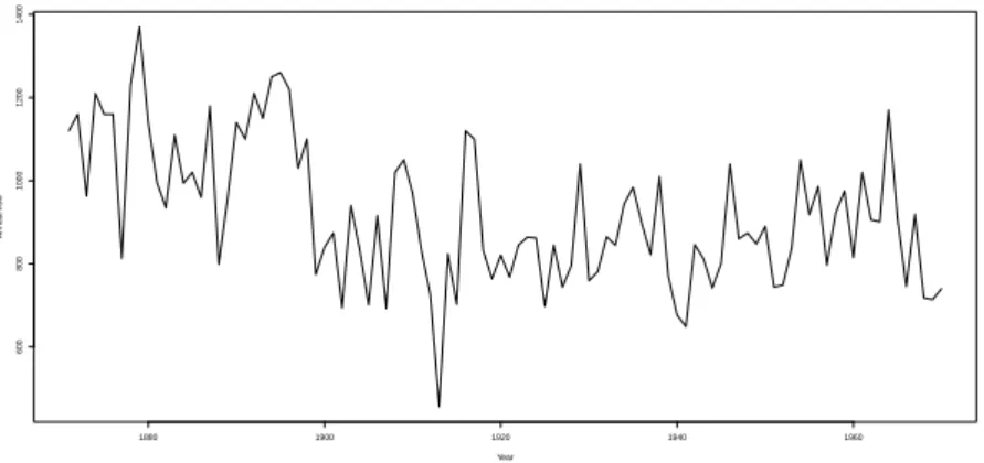
Year Ann ual flo w 1880 1900 1920 1940 1960 600 800 1000 1200 1400
Figure 1.1.:Annual flow (in 108m3) of the river Nile at Aswan from 1871 to 1970.
1.2 Change-point analysis under nonparametric regression
A large body of papers consider the nonparametric regression problem in (1.2) and assume that the regression function mis element of some function class containing only global smooth functions. Typical examples are the function classes in (1.3) – (1.5). It is often justifiable to assume that such a global smoothness of the regression function cannot hold for specific datasets. Consider Figure 1.1 for instance, where the annual flow of the Nile is displayed for the time from 1871 to 1970. Cobb (1978) pointed out that there is an apparent change-point visible around the year 1898, so that it is not appropriate to model the data with a regression function which is smooth over the whole domain. In addition, classical estimation procedures such as kernel smoothing, local linear fitting or wavelet estimation are not longer optimal in the presence of change-points without essential amendments.
Interpretation of a change-point
The first work in a regression setting with discontinuities interpreted as change-points is due to Thistlethwaite and Campbell (1960). Ever since change-points have attracted much attention in the research and many scientific articles from diverse academic disciplines dealt with problems of a change-point nature. As a consequence there have evolved different possibilities to declare what a change-point is. Casually speaking, a change-point of a function f is any point where f changes its local behavior suddenly and drastically. The most prevalent definition of a change-point is declaring it as a point of discontinuity in the function of interest, though this is quite not the only option. Discontinuities in the derivatives of the function of interest are as well points with potential strong impacts on the behavior of the function, e.g. a jump discontinuity in the first derivative would relate to an abrupt change in the direction of the regression function, while a jump discontinuity in the second derivative describes a sudden change in the curvature. Such an irregularity will be called aγ-kinkor a kink of orderγ, that is a jump in theγ-th derivative of the regression function. Generalizations of these kinks in a Hölder sense areγ-cusps, i.e. forγ >0,a function f :Rd→Rhas aγ-cusp at some
pointθ∈Rd, if there exists some finiteC>0 such that
|f( bγc)(θ+h) −f( bγc)(θ)| ≥C||h||γ− bγc,
ashtends to zero. Another type of change-points are so-calledpoints of rapid changeconsidered by Menéndez et al. (2010), which are points with a rapid but smooth change occurring due to a local maximum of the first derivative with a certain magnitude.
1.2. Change-point analysis under nonparametric regression 15
by a curve, so that one rather speaks of achange-curve. We will sometimes abuse the denotations and simply refer to change-curves also as change-points for sake of brevity when speaking about change-point problems in nonparametric regression of arbitrary dimension.
Statistical challenges for change-point analysis
Initially, it is important to envision the numerous statistical issues arising in the context of NPP with change-points. Firstly, an obvious question is whether the unknown regression function is globally smooth or has some change-points, which naturally leads to estimation of the numbers of such change-points. This task is called change-point-detection. Secondly, given the existence of change-points, the explicit estimation of change-point-locations is of major interest. Thirdly, besides mere location of the change-point it is worthwhile to estimate the change-point-magnitude, such as the jump-height, to quantify the impact of the change-point on the considered function. Fourthly, having a reasonable believe that change-points are present and given reliable estimates for the three latter statistical tasks, the estimation of the (regression) function itself with incorporation of the change-points volunteers. The focus of this thesis lies strongly on the second issue and consequently the review of the literature will be mainly concentrated on this topic. For the other issues see the monograph by Qiu (2005) for further reading.
1.2.1 Estimation of change-point-locations in univariate frameworks
In the following we give a brief overview on the different methods, considered models and especially the coherences between the various frameworks in the literature about NPP with change-points. From now on we denote the regression function as mθ to emphasize with the parameterθ that possibly change-points may be present.
Maximum-likelihood estimation
Ibragimov and Has’ Minskii (1981) considered the regression function mθ(x)= 1x≤θ for some
unknownθ ∈ (0,1)in the white noise model (WNM). This is a parametric regression model with a single jump-locationθ.They showed that the maximum-likelihood estimate ˆθM LEofθconverges with the rate2.In addition, it was shown that−2(θˆM LE−θ)converges in distribution with distributional limit
Z0=arg max u∈R
B(u) − |u|/2, (1.8)
whereB is a two-sided Wiener process. For the related parametric regression problem withmθ as before and different design assumptions, Korostelev and Tsybakov (1993) obtained the convergence rates of the least-squares estimate ˆθLS which coincides with the maximum-likelihood estimate for Gaussian errors. In case of equidistant design there is an asymptotically non-negligible bias of orderO(n−1), whereas for the random design the bias is asymptotically negligible. In the latter case the distributional limit of n(θˆLS−θ)is the discrete version of (1.8). Hinkley (1970) derived the asymptotic of the maximum-likelihood estimate by considering the mean-change problem in a sequence of Gaussian random variables which is basically the NPP for a fixed regular design and Gaussian errors. Korostelev (1987) verified for the jump-location estimation the minimax rate of convergence to be of orderO(2)in a WNM over a function class which is Lipschitz continuous away from the single discontinuity. By means of the usual correspondence this result can be transferred to a NPP which leads to a minimax rate of orderO(n−1).Thus, higher smoothness assumptions on the regression function away from the jump do not affect the minimax rate of convergence.
Smoothed difference approach
A typical assumption made in the univariate NPP with change-point is that the regression function (or itsγ-th derivative) is of the form
m(θγ)(x)=m(x)+ k
Õ
i=1
ai1[θi,∞), γ∈N∪ {0}, (1.9)
wherem:D→Ris a smooth function,θ=(θ1,. . .,θk) ∈Dkare the change-point-locations andai,0,
i=1,. . .,k the corresponding change-point-magnitudes. Note that for the casek=0 the regression function (or its derivative) is smooth as well. Depending on this representation a popular method for estimating such change-point-locations in a univariate setting is to consider smoothed left- and right-sided limits ofm(θγ), say ˆm(nγ,)−and ˆm
(γ)
n,+and define an M-criterion function as the difference of both one-sided-smoothers. This method is called thesmoothed difference approach. An estimate of the change-point-magnitude is naturally given by the value of the contrast function at its maximizer or minimizer. Note that the smoothed difference approach method volunteers for the detection of a change-point as well, by deciding that the change-point estimate is tagged as a change-point if the estimate of the change-point-magnitude exceeds a certain threshold (see Müller and Stadtmüller (1999) or Porter and Yu (2015) and their references for further reading). A related method based on weighted three smoothers, namely left- and right-sided smoothers and a central smoother, was considered by McDonald and Owen (1986) and Hall and Titterington (1992).
Most of the works using a smoothed difference approach differ by the assumptions onm,the smooth part of the regression function in (1.9), as well as the used one-sided smoothers, which will be pointed out in the following. Yin (1988) estimated change-points by means of a difference of one-sided averages in a WNM with unknown number of jumps. Qiu and Li (1991) considered in a NPP with fixed design differences of one sided-kernels as a contrast function to estimate jumps in the regression function, while Müller (1992) extended this method to estimate jump-point-locations and also kink-locations of higher order. In the same model with several jump-points, where the number of jumps is unknown, Wu and Chu (1993) used different types of kernels for the contrast function to estimate jump-location and -height as well as to give a procedure to estimate the number of jumps based on sequential hypothesis testing. Both latter papers obtained asymptotic normality of their jump-location estimate and their jump-magnitude estimate, while Müller (1992) also derived asymptotic normality of odd centered moments of his kink-location estimator. In Müller (1992) the one-sided kernels are supposed to vanish at zero, which in combination of an undersmoothing resulted in an unbiased asymptotic normality of the jump-location-estimates but with a sub-optimal rate of convergence and rather strong assumptions on the regression function. For weaker assumptions on the regression function, but with Gaussian errors and assuming that the change-point is one of the design points, Loader (1996) obtained the optimal rate by using differences of local polynomial smoothers as a criterion function and by letting the difference be strictly positive at zero. In order to derive the optimal rate of convergence Loader (1996) determined the asymptotic distribution of the estimate, which is a discrete version of (1.8). By assuming that the change-point is one of the design points the usually asymptotic non-negligible bias becomes negligible.
Based on a semi-parametric approach, which is asymptotically related to Müller (1992), Eubank and Speckman (1994) estimated a single kink-location and kink-magnitude of first order and obtained asymptotic normality of their estimates. Müller and Song (1997) and Gijbels et al. (1999) suggested two-stage estimation procedures which attain the optimal rate of convergence for the jump-location. In the first step, both defined a pilot estimate for an interval where the jump-location is located with high probability, while in the second step a refined estimate for the jump-location based on the first step is introduced by using a smoothed difference approach. Grégoire and Hamrouni (2002) considered the NPP with random design and used the difference of local linear smoother from left
1.2. Change-point analysis under nonparametric regression 17
and right as the criterion function. For a specific standardization of their M-estimate they obtained its asymptotic distribution, which is the maximizer of a compounded Poisson process, and also asymptotic normality of their jump-height estimate. Prieur (2007) obtained comparable results for a design with dependency structure, while Lin et al. (2008) also considered kink-location estimation of higher order and established asymptotic normality of exponents of their estimates.
Wavelet based methods
Another commonly used approach is based onwavelet transformationof the regression function as a criterion function. Wang (1995) suggested a wavelet transformation of the signal in a WNM with unknown number ofγ-cusps of the underlying function to detect such cusps. The rate for estimation a γ-cusp with this technique is of orderO((2log()−η)1/(2γ+1))for someη >0. Raimondo (1998) derived the minimax rates of convergence for the estimation of the γ-cusp-location for function classes which have one singleγ-cusp and are Hölder-smooth away from it. In addition, he provided a wavelet transformation based method to achieve his claimed minimax rate. He claimed that the minimax rate is of orderO(n−1/(2γ+1)),which is in fact true forγ ∈ [0,1/2),but not forγ ≥1/2 as shown by Goldenshluger et al. (2006).
Luan and Xie (2001), Park and Kim (2004) as well as Park and Kim (2006) considered basically the same estimates based on wavelet transformation as in Wang (1995) respectively Raimondo (1998) with different model assumptions for the NPP such as random design or some dependency structure in the errors and obtained the rate of convergence of order O(n−1/(2γ+1)) for their cusp-location estimates. Furthermore, Huh and Carriere (2002) extended the approach of Loader (1996) to a kink of orderγ estimation problem but without assuming Gaussian errors. They derived for their kink-location estimate the asymptotic distribution which is a generalized and discrete version of (1.8). However, all aforementioned procedures were out to attain the wrong minimax rates of Raimondo (1998) so that these methods are sub-optimal forγ >1/2.
Zero-crossing time technique
A further popular method in the literature on image processing and change-point analysis is the so-calledzero-crossing-time-technique. This name comes from using a Z-criterion function which is a smoothed second derivative of the object of interest. The motivation of this approach is that provided the function of interest has a jump-location, say atθ,a smoothed version of the function will have a large slope nearθ,so that its first and second derivatives have a local maximum respectively a zero nearθ.
Thus, for an appropriate kernel functionK:R→R, specified roughly below, the considered criterion
function is ψh,m(t)=h−(γ+1) 1 ∫ 0 K(γ+2) h−1(x−t) m(x)dx, (1.10)
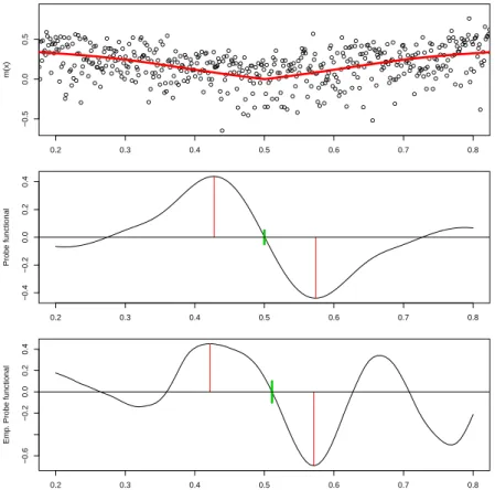
whereh>0 is a bandwidth parameter andγ∈N∪ {0}.Now, the kernelKis chosen such thatψh,m has a well separated zero with a global maximum and a global minimum left respectively right from the zero and in addition, the zero of ψh,m is close to the discontinuity of m(γ),see Figure 1.2 for illustration purposes. Chapter 3 provides more details about the particular choice of the kernel, as it is fundamental for the evolved theory in that chapter. An empirical Priestley-Chao-type of the criterion function is given by
ˆ ψn,h(t)=n−1h−(γ+1) n Õ i=1 YiK(γ+2)(h−1(xi−t)). (1.11)
● ● ● ● ● ●● ● ● ● ●● ● ● ● ● ● ● ●● ● ● ● ●● ● ● ● ● ● ● ● ● ● ● ● ●● ● ● ● ● ● ● ● ●● ● ● ● ● ● ● ● ● ● ● ● ● ● ● ● ● ● ● ● ● ● ●● ●● ● ●● ● ● ● ● ● ● ● ● ● ● ● ● ● ● ●● ●● ● ● ● ● ●● ● ● ● ●● ● ● ● ●● ● ●● ● ● ● ● ● ● ● ● ●● ● ● ● ● ● ● ● ● ● ● ● ● ● ● ● ● ● ● ● ● ● ● ● ●● ● ● ●● ● ●● ● ● ● ● ● ● ● ● ● ● ● ● ● ●● ● ● ● ● ● ● ● ● ● ● ●● ● ● ● ● ● ● ● ● ● ● ● ● ● ●● ● ●● ● ●● ● ● ● ●●● ● ● ● ●● ● ● ● ● ● ● ●● ● ● ● ● ● ● ● ● ●●●● ● ● ● ● ● ●● ●● ● ● ● ● ● ● ● ● ● ● ● ● ● ● ●● ● ● ● ● ● ● ● ● ● ● ●● ● ● ● ● ● ● ● ● ● ● ●● ● ● ● ● ● ● ● ● ● ● ● ●● ● ● ● ● ● ● ● ● ● ● ● ● ● ● ● ● ● ● ● ● ● ● ● ● ● ● ● ● ● ● ●● ● ● ● ●●● ● ● ● ● ● ●● ● ● ● ●● ● ● ● ●● ● ● ● ●● ● ● ● ● ● ● ● ● ● ● ● ● ● ● ● ● ● ● ● ● ● ● ● ● ● ● ● ● ● ● ● ● ● ● ● ● ● ● ●● ● ● ● ● ● ● ● ● ● ●● ● ●● ● ● ● ● ●● ● ● ● ● ●● ● ● ● ● ●● ● ● ● ● ●● ● ● ●● ● ● ●● ●● ● ● ● ● ● ● ●●●● ● ● ● ● ● ● ● ● ● ● ● ● ● ● ● ● ●● ● ● ● ● ● ● ● ● ● ● ● ● ● ● ● ● ● ● ● ● ● ●● ● ● ●●● ● ● ● ● ● ● ● ●● ● ●●● ● ●● ● ●● ● ● ● ●●●●● ●● ● ● ● ● ● ● ● ● ● ● ● ● ● ● ● 0.2 0.3 0.4 0.5 0.6 0.7 0.8 −0.5 0.0 0.5 m(x) 0.2 0.3 0.4 0.5 0.6 0.7 0.8 −0.4 −0.2 0.0 0.2 0.4 Probe functional 0.2 0.3 0.4 0.5 0.6 0.7 0.8 −0.6 −0.2 0.0 0.2 0.4 Emp . Probe functional
Figure 1.2.:Illustration of the zero-crossing-time-technique for a kink of first order. Top plot: Regression function with a single kink and noised observations. Middle plot: Corresponding criterion function in (1.10). Bottom plot: Empirical version in (1.11).
The advantage of this approach is that the global extreme values often allow a more accurate location of a change-point than other change-point-location methods.
Goldenshluger et al. (2006) estimated single jump-locations in an indirect WNM by using a zero-crossing-time-technique. Moreover, they derived the minimax lower bound for this estimation problem for Sobolev-smooth as well as analytical functions except for a single jump. This minimax lower bound can be related to the NPP with fixed design and in particular imply that the minimax rate of Raimondo (1998) is not correct for γ ≥1/2,since the rate of convergence is driven by the smoothness of the regression function outside the cusp. Although their method is rate-optimal, it is not apparent how to apply the method for a direct nonparametric regression model with equidistant design. For this issue Cheng and Raimondo (2008) modified the method of Goldenshluger et al. (2006) by constructing kernels for their probe functional which is a smoothed version of the third derivative of the regression function for the purpose of kink-detection for kinks of first order. Goldenshluger et al. (2008a) and Goldenshluger et al. (2008b) embedded respectively extended the results of Goldenshluger et al. (2006) to a periodic setting and cover derivative estimation, convolution as well as delay and amplitude estimation, while Goldenshluger et al. (2008b) constructed adaptive estimators based on Lepski’s adaption scheme.
The work of Wishart (2009) extended the method used in Cheng and Raimondo (2008) to the direct fractional-white-noise-model and the nonparametric regression model with equidistant design and dependency structure in the error, while Wishart (2011) established a minimax lower bound for this framework for slightly different function classes. For a random design in a similar framework, where the design follows some long-range dependency structure, Wishart and Kulik (2010) obtained rate of convergence which seem to be optimal.
1.2. Change-point analysis under nonparametric regression 19
Other methods
Finally, there are approaches worth noting which do not fit into the aforementioned categories, e.g. jump detection based on Fourier analysis was deployed by Lombard (1988). Dempfle and Stute (2002) considered the univariate NPP in a random design with very lax assumptions and defined a criterion function based on empirical quantiles to obtain an estimate which converges with the optimal rate.
1.2.2 Estimation of change-point-locations in multivariate frameworks
For the multivariate NPP with change-curves a prevalent model is the boundary fragment model, which is given by settingD=[0,1]dand
Yi1,...,id=mφ(xi1,...,id)+εi1,...,id, i1,. . .,id∈ {1,. . .,n}, mφ(x)=m(x)+τ(x)1G(φ),
G(φ)={(x1,. . .,xd) ∈D|0≤xd≤φ(x1,. . .,xd−1)}
(1.12)
wherem:D→Ris a smooth curve,φ:[0,1]d−1→ (0,1)the jump-location-curve andτ:D→
R+ the corresponding jump-height-curve. This model is motivated by considering small parts of the original image (and further rescaling), where some smooth edgeφis located.
Korostelev and Tsybakov (1993) provided minimax results for jump-location-curves in Hölder-smoothness classes as well as a rate-optimal procedure for a random design based on piecewise-polynomial estimation on partitions of the design domain. The optimal rate of convergence depends only on the smoothness of the jump-location-curve and is not affected by additional smoothness of the smooth partmin (1.12), also referred to as anuisance parameter. Moreover, for a regular fixed design withnddesign points, the minimax rate can not be faster thann−1because of the dominating bias, so that the optimal rate is even not affected by additional smoothness assumptions on the jump-location-curve.
Rotated difference kernel estimation
Multivariate extensions of the idea of using differences of one-sided smoothers were introduced by Müller and Song (1994) and Qiu (1997) with the so-calledrotational difference kernel method. This method allows to rotate the support of the corresponding one-sided kernels in order to adjust the criterion function such that its value is large near a change-curve. Garlipp and Müller (2007) pointed out that for the resulting estimates the order of scaling and rotating of the kernel support is important. We define the rotational difference kernel method for the bivariate version of the boundary fragment model in (1.12). Firstly, define the rotation matrix
Dψ= cos(ψ) sin(−ψ) sin(ψ) cos(ψ) , ψ∈R. (1.13)
Secondly, for a bandwidthh>0 andz=(z1,z2)T ∈R2consider the rotated difference kernel K(z;ψ,h)=K(h−1D−ψz)/h2
whereK(z)=K(z1,z2)=K1(z1)K2(z2)is a product kernel of univariate kernel functionsK1andK2, whereK2 is odd and justifies the term "difference". Finally, forz∈ [0,1]2 andψ∈ [−π/2,π/2] the
contrast process with Priestley-Chao-type weights is defined as ˆ Mn(z;ψ,h)=n−2 n Õ i1,i2=1 Yi1,i2K(z−xi1,i2;ψ,h). (1.14)
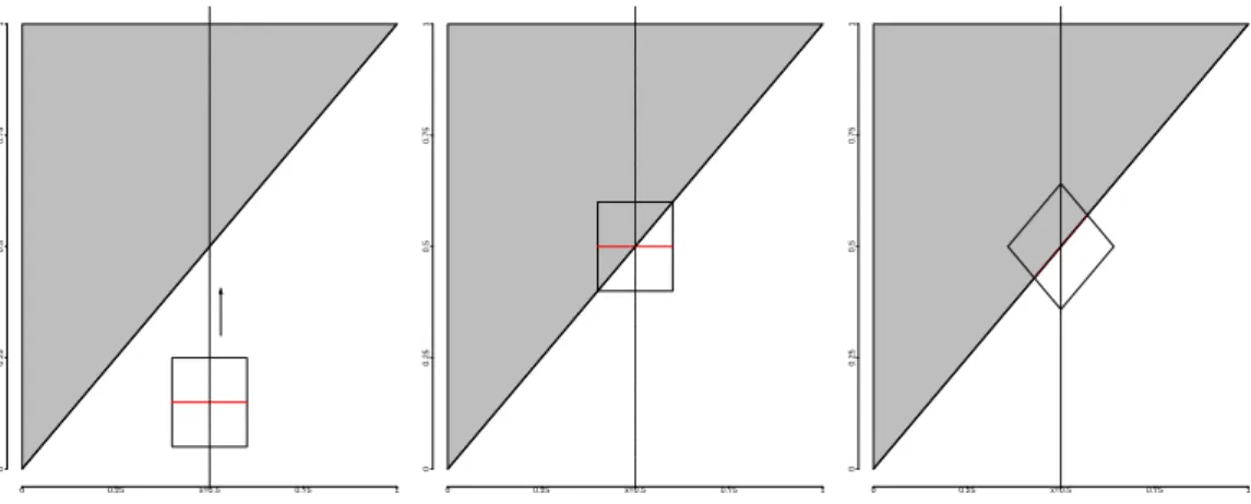
For anx∈ (0,1)denote byψ(x)=arctan(φ0(x))the slope of the tangent atφ(x). An estimator for the bivariate parameter φ(x),ψ(x) is then given by ˆ φn(x),ψˆn(x) ∈ arg max y∈[h,1−h],ψ∈[−π/2,π/2] ˆ Mn((x,y)T;ψ,h). (1.15) An illustration of the mechanism of the M-estimates in (1.15) is given in Figure 1.3. For some fixed x the largest contrast along the stripe x× (h,1−h) is sought by rotating the kernel window appropriately. The line within the kernel window indicates along which direction the difference is considered. An estimator for the jump-height at xis given by
ˆ τn(x)=Mˆn((x,φˆn(x))T; ˆψn(x),h). (1.16) 0 0.25 0.5 0.75 1 0 0.25 x=0.5 0.75 1 0 0.25 0.5 0.75 1 0 0.25 x=0.5 0.75 1 0 0.25 0.5 0.75 1 0 0.25 x=0.5 0.75 1
Figure 1.3.:Illustration of rotated difference kernel estimation for a linear jump-location-curve.
Other methods
A bivariate extension of the wavelet transformation technique of Wang (1995) for the NPP with equidistant design and Gaussian errors is given in Wang (1998). Another access to the multivariate NPP with change-curves is by treating the jump-location-curve as a pointset and consequently estimate it by a point set. This idea is motivated from developments in the image processing literature and the focus lies often on the detection of change-points. Qiu and Yandell (1997) suggested an algorithm to detect change-points by fitting local linear planes in the neighborhood of design points for the bivariate case, which was modified and extended to the three dimensional case in Mukherjee and Qiu (2011). Qiu (2002) proposed the simplified rotational difference kernel method for the detection of the jump-location-curve, while Sun and Qiu (2007) considered a criterion function based on estimation of first- and second-order-derivatives by local quadratic kernel smoothing. Moreover, Qiu (2002) showed that the rotational difference kernel can be related to the Sobel edge detector which is popular in the realm of image processing. For a review on the literature on image processing consider Qiu (2005) or Sonka et al. (2014).
1.3. Uniform M- and Z-estimation theory 21
1.3 Uniform M- and Z-estimation theory
As we have seen in the preceding section, many of the popular estimation procedures in the change-point analysis are simply M- or Z-estimates. In this section, M- and Z-estimation are introduced in two more general settings which firstly extend the classical theory for M- and Z-estimation and secondly will be highly relevant for the concepts in the further chapters. The setting is as general as possible and is therefore not restricted to the nonparametric regression framework.
1.3.1 Uniformity over the function class
Suppose the object of interest is a parameterθf of a function f ∈ F with F ={f :I→R| f has some unique property inθf ∈Θ},
whereΘ⊂ I is a compact subset andI ⊂Rd is some set. In view of change-point problems it is evident that the parameterθf corresponds to a change-point. The considered statistical setting often allows to define for any f ∈ F a(Z-)criterion function
Rd× F →R
(x,f) 7→ψ(x;f),
such that the parameter of interestθf is a zero ofψ(·;f),. In order to estimate this parameter one might try as an estimate ˆθna zero (provided it exists) of anempirical (Z-)criterion function
Ω×Rd→R (ω,x) 7→ψˆn(ω,x),
where we in the following suppress the dependency onω and simply write ˆψn(x). We could also define an M-estimate in the same manner, but as we only need a Z-estimate in the further chapters we content ourselves with the explicit definition of Z-estimates in the above framework.
Asymptotic analysis
Assuming that the convergence of the empirical criteria function against the asymptotic criteria function holds uniformly in probability over the function class it is reasonable to believe that the corresponding Z-estimates converge to the actual parameter in probability and uniformly over the function class, provided the parameter of interest is somehow unique for the criterion function. Indeed, this heuristic is fruitful if the parameter θf is a well-separated zero, as the following proposition shows.
Proposition 1.1. Letψˆn:Rd→Rbe random functions and letψ:Rd× F →Rbe a deterministic function. Suppose that
sup
θ∈Θ
|ψˆn(θ) −ψ(θ;f)|=oP,F(1), (1.17) and that there exists a family(θf)f∈ F⊂Θsuch that for any >0
inf
f∈ F θ∈I:| |θinf−θf| |∞≥
Then, for any estimatorθˆnwithθˆn∈Θandψˆn(θˆn)=oP,F(1)it holds that |θˆn−θf|=oP,F(1).
Proof of Proposition 1.1. With (1.17) and the properties of ˆθnit follows that for anyδ >0
Pf(|ψ(θˆn;f)|> δ) ≤Pf(|ψˆn(θˆn)|> δ/2)+Pf(|ψˆn(θˆn) −ψ(θˆn;f)|> δ/2) ≤oF(1)+Pf(sup
θ∈Θ
|ψˆn(θ) −ψ(θ;f)|> δ/2)=oF(1).
Given >0 chooseη >0 as the left side of (1.18). Then,
Pf(|θˆn−θf|> ) ≤Pf(|ψ(θˆn;f)| ≥η)=oF(1).
A remark on the conditions (1.17) and (1.18) is given in the succeeding subsection.
Having verified consistency of the estimates, a natural question arising is iftn(θˆn−θf)converges in distribution to a non-degenerate limit for a suitable sequence of real-values(tn)n⊂R+.Fortunately, the nature of Z-estimates yields a convenient way for answering this question in case of a smooth criterion function. For sake of simplicity assume thatd=1,i.e. ˆψnis one-dimensional as well as that
ˆ
ψnis two-times differentiable and ˆψ
(1)
n is not zero in a certain neighborhood ofθf, a Taylor expansion of ˆψnaroundθf yields
0=ψˆn(θˆn)=ψˆn(θf)+(θˆn−θf)ψˆ
(1)
n (θ˜n,f),
where ˜θn,f is betweenθf and ˆθn.Rearranging terms in the preceding display and multiplying bytn leads to tn(θˆn−θf)=−tnψˆn(θf) ψˆ (1) n (θ˜n) −1, (1.19) provided ˆψn(1)(θ˜n) −1
exists. The termtnψˆn(θf)is called the(rescaled) score. For a fixed function
f it is possible to derive the asymptotic distribution as in the classical Z-estimation framework, see Section 5.3 in van der Vaart (2000). Though to obtain a stronger result, as for instance
sup f∈ F
|Pf(tn(θˆn−θf) ≤x) −F(x)|=o(1), ∀x∈Rd
whereFis some (known) cumulative distribution function, the results in part C of the appendix are helpful as well as Proposition 1.1. A specific application is given in Chapter 3.
1.3.2 Uniformity over the covariate space
In many statistical problems one has the following setting. Θ⊂Rk is compact and I ⊂
Rd is some
subset, the covariate space. Furthermore, one is interested in estimation of f :I→Θuniformly over the covariate space I. Fortunately, the statistical setting frequently allows to define a(M-)criterion function
Θ×I→R