Bayesian logistic regression models for credit scoring

(1)

1

Bayesian Logistic Regression Models for Credit Scoring

by

Gregg Webster

A thesis submitted to Rhodes University in partial fulfilment of the

requirements for the degree of

Master of Commerce

in

Mathematical Statistics

December 2011

(2)

2 DECLARATION

Except for references specifically indicated in the text, this study is my own work and has not been submitted elsewhere for degree purposes.

(3)

3

Abstract

The Bayesian approach to logistic regression modelling for credit scoring is useful when there are data quantity issues. Data quantity issues might occur when a bank is opening in a new location or there is change in the scoring procedure. Making use of prior information (available from the coefficients estimated on other data sets, or expert knowledge about the coefficients) a Bayesian approach is proposed to improve the credit scoring models. To achieve this, a data set is split into two sets, “old” data and “new” data. Priors are obtained from a model fitted on the “old” data. This model is assumed to be a scoring model used by a financial institution in the current location. The financial institution is then assumed to expand into a new economic location where there is limited data. The priors from the model on the “old” data are then combined in a Bayesian model with the “new” data to obtain a model which represents all the available information. The predictive performance of this Bayesian model is compared to a model which does not make use of any prior information. It is found that the use of relevant prior information improves the predictive performance when the size of the “new” data is small. As the size of the “new” data increases, the importance of including prior information decreases.

(4)

4

Acknowledgements

Thank you to my parents, Robert and Debra Webster for their constant love and support throughout my studies. This research is dedicated to them.

Thank you to my supervisor, Professor Sarah Radloff for her guidance throughout my research. Your helpfulness and support is highly appreciated.

Thank you to my friends and family for their support and input. Another thank you goes out to all the staff and students of the Rhodes Statistics department. A particular thank you goes to Tafadzwa Mutengwa for all the help, laughs and hard work we did together.

This research was possible through the assistance from the Henderson Rhodes University Prestigious Scholarship and is hereby acknowledged.

(5)

5

LIST OF FIGURES

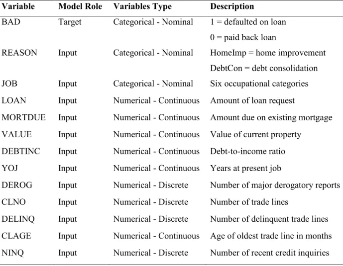
Fig. 4.1 Bar plots of REASON and JOB………..53

Fig. 4.2 Histogram and Box plot of LOAN……….53

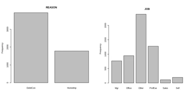
Fig. 4.3 Histogram and Box plot of MORTDUE……….54

Fig. 4.4 Histogram and Box plot of VALUE………...54

Fig. 4.5 Histogram and Box plot of DEBTINC………...54

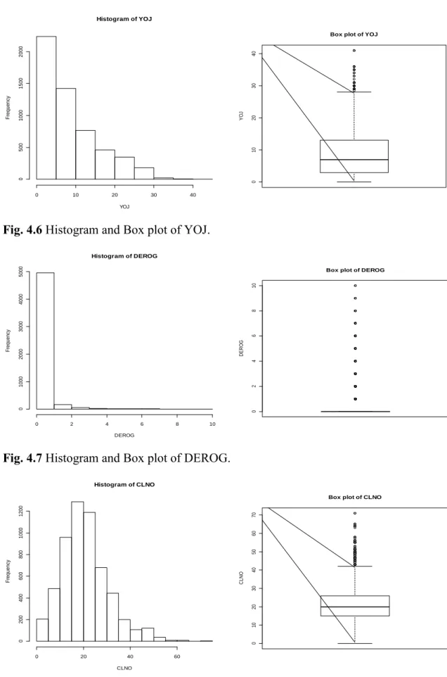
Fig. 4.6 Histogram and Box plot of YOJ……….55

Fig. 4.7 Histogram and Box plot of DEROG………...55

Fig. 4.8 Histogram and Box plot of CLNO………..55

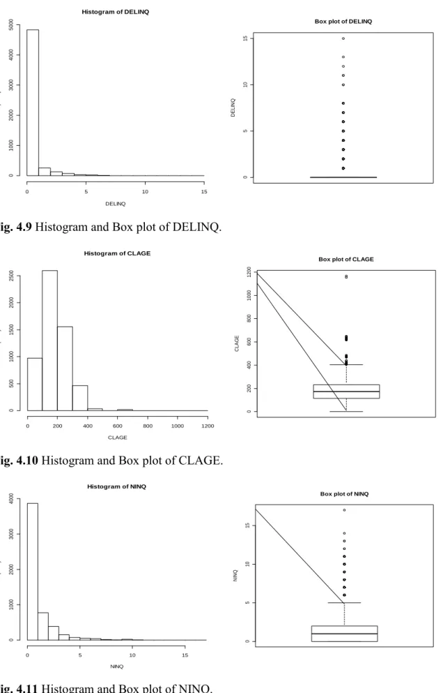
Fig. 4.9 Histogram and Box plot of DELINQ………..56

Fig. 4.10 Histogram and Box plot of CLAGE……….56

Fig. 4.11 Histogram and Box plot of NINQ………56

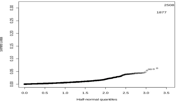
Fig. 4.12 Half-normal plot of residuals for the “old” data………...61

Fig. 4.13 Half-normal plot of leverages for the “old” data………..62

Fig. 4.14 Half-normal plot of the Cook’s distance statistics for the “old” data………..62

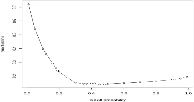
Fig. 4.15 Optimal cut-off probability when total error is minimized………...65

Fig. 4.16 Optimal cut-off probability when error function is minimized with α = 0.8………65

Fig. 4.17 Half-normal plot of residuals for the “new” data……….70

Fig. 4.18 Half-normal plot of leverages for the “new” data……….70

Fig. 4.19 Half-normal plot of the Cook’s distance statistics for the “new” data……….71

Fig. 4.20 Trace and density plots of the posteriors for the first four variables using an informative prior………..77

(9)

9 Fig. 4.21 Trace and density plots of the posteriors for the first four variables using a

non-informative prior………..80 Fig. 4.22 Error rates of Models 1, 2 and 3 when the models are trained using differerent

sampler sizes and the cut-off probability is 0.3………...88 Fig. 4.23 Error rates of Models 1, 2 and 3 when the models are trained using differerent

(10)

10

LIST OF TABLES

Table 3.1 Classification table of the predictive performance of the logistic regression

model………...29

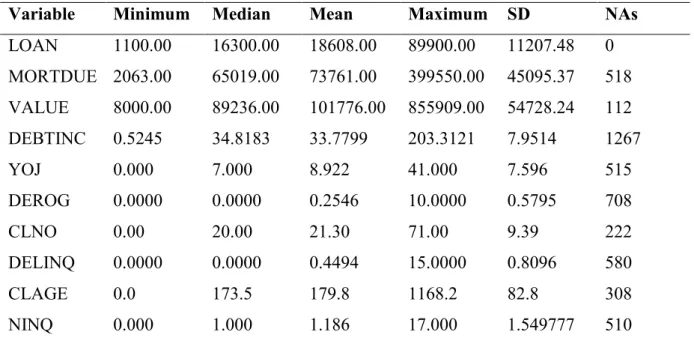
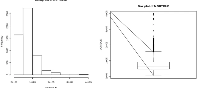
Table 4.1 Variable type and description for each variable in the data set………...51

Table 4.2 Summary statistics for the numerical input variables………..52

Table 4.3 Logistic regression model fitted on the “old” data………..58

Table 4.4 Correlation matrix of numerical independent variables on the “old” data………..60

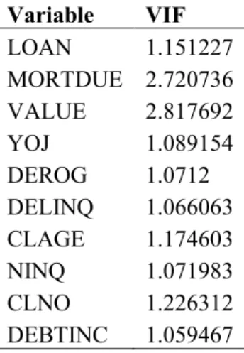
Table 4.5 Variance inflation factors (VIF) of numerical independent variables on the “old” data………..61

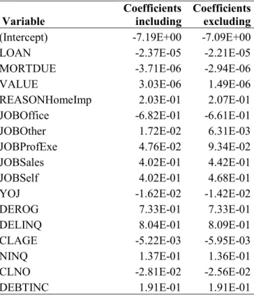
Table 4.6 Comparison of model coefficients when possible leverage and influential observations are either included or excluded from the “old” data………...63

Table 4.7 Logistic regression model fitted on the “new” data………66

Table 4.8 Correlation matrix of the numerical independent variables on the “new” data…...68

Table 4.9 Variance inflation factors (VIF) of numerical independent variables on the “new” data………...69

Table 4.10 Comparison of model coefficients when possible influential observations are either included or excluded from the “new” data………....72

Table 4.11 Logistic regression model on “new” data with influential observations removed………...73

Table 4.12 Prior parameters for an informative Bayesian logistic regression model………..74

Table 4.13 Bayesian logistic regression model on the “new” data with an informative prior……….75

Table 4.14 Geweke diagnostic statistics for each variable of the Bayesian logistic regression model with informative prior………...78

Table 4.15 Bayesian logistic regression model with non-informative prior on the “new” data………...79

Table 4.16 Geweke test statistics for each variable for the Bayesian logistic regression model with non-informative prior………...81

(11)

11 Table 4.17 Classification table for the logistic regression model with cut-off probability of

0.3………82 Table 4.18 Classification table for the Bayesian logistic regression model with informative

prior and cut-off probability of 0.3………...82 Table 4.19 Classification table of the Bayesian logistic regression model with

non-informative prior and cut-off probability of 0.3………...83 Table 4.20 Comparison of Models 1, 2 and 3 when the cut-off probability is 0.3…………..83 Table 4.21 Classification table of logistic regression model with cut-off probability of

0.48………...84 Table 4.22 Classification table of Bayesian logistic regression model with informative prior

and cut-off probability of 0.48……….85 Table 4.23 Classification table of the Bayesian logistic regression model with

non-informative prior and cut-off probability of 0.48………....85 Table 4.24 Comparison of Models 1, 2 and 3 when the cut-off probability is 0.48…………86

(12)

12

Chapter 1: Introduction

1.1 Context of the Research

Consumer credit is one of the main driving forces which allowed for the rise (and possible demise) of most of the leading industrialized countries. The growth in home ownership and consumer spending over the last 50 years would not have occurred without credit. When a financial institution grants credit to an applicant the financial institution trusts the applicant to pay back the credit. The applicant may, however, default on payments back to the institution. It is the task of the financial institution to make sure that the number of defaults is minimized so that risk is reduced. This is done by screening the applicants when they apply for credit. Scoring methods are used to estimate the credit worthiness of an applicant. These credit scoring methods estimate the probability that an applicant will default or become delinquent. Credit scoring methods use statistical methods based on historical credit data to build a model which predicts whether an applicant will default or not. The financial institution can then use the model to decide whether or not to grant credit to the applicant also considering how much risk the institution is willing to take on. As mentioned, building a credit scoring model requires the use of historical data. There may, however, be situations when there is limited historical data. This might occur when the financial institution is expanding into a new economic location (country) and no data is available at first. Data quantity issues might also occur when there is a change in the scoring procedure. In these situations it is difficult to build a good scoring model as there is initially not enough data available. Thus, expert information can be important. An existing reliable generic scoring model may be available at first which could be used for scoring. This generic scoring model could then be modified as new data becomes available. Institutions already using scorecards may be able to combine their expert knowledge with new sources of information to obtain improved scoring models. In order to do this, a Bayesian approach is proposed where the expert knowledge is combined with the limited amount of data. The aim is to see whether the combination of expert knowledge with data gives a better model than one that uses only the limited amount of data.

(13)

13 The scope of Bayesian inference has greatly improved since it was discovered that Markov Chain Monte Carlo (MCMC) Methods could be used to sample from the posterior distributions. The general MCMC algorithm is called the Metropolis-Hastings (MH) algorithm.

1.2 Objectives of the Study

The objectives of this study are as follows:

- Investigate credit scoring and the associated problems - such as reject inference.

- Introduce the concepts and methods of the Bayesian logistic regression models for credit scoring. This includes an in-depth explanation of the Markov Chain Monte Carlo (MCMC) methods.

- Develop a standard logistic regression scorecard.

- Develop a Bayesian approach to the scorecard for when the bank enters a new market or there is a change in procedure.

- Compare the Bayesian approach to the standard logistic regression approach. This would involve comparing the models’ predictive powers on a test set.

- Make recommendations on the Bayesian approach to credit scoring.

1.3 Organization of the Study

Chapter 2 gives the history of credit scoring, problems with credit scoring and examines previous research on models used for credit scoring. The chapter provides a literature review on the models used for credit scoring focusing on the Bayesian logistic regression models. Chapter 3 examines the methods used in detail; it provides derivations and proofs of key results in order to gain an understanding of the models used. In Chapter 4 the results of the data analyses are presented and discussed. Chapter 5 summarizes the study, gives limitations and discusses areas for further research.

(14)

14

Chapter 2: Literature Review

2.1 History of Credit Scoring

Credit scoring is essentially a classification problem where applicants are classified into different groups. According to Thomas (2009) statistical classification techniques started when Fisher (1936) developed one of the first successful classification models to classify three different types of the iris flower. He used different physical measurements of the flower to discriminate between the three types of Iris flowers. Durand (1941) was then the first to recognise that these statistical classification techniques could be used to classify good and bad loans. Before this, Thomas (2009) states that financial institutions based decisions on whether to grant credit subjectively. When credit cards were introduced in the 1960s, the usefulness of credit scoring started to be realized. Because of the large number of people applying for credit cards, automation of the credit application procedure seemed to be the only solution. When the financial institution introduced the credit scoring model they found that the model performed a lot better than the previous (subjective) judgment scheme. The result was that, as Thomas (2009) states, default rates dropped by 50% or more. In the 1980s the success of credit scoring in credit cards meant that financial institutions started using scoring methods for other products too such as personal loans, home loans and business loans.

The subprime mortgage crisis caused a global recession in 2007. This crisis proved that financial institutions did not fully understand the risks they were taking on. According to Rona-Tas and Hiß (2008) a credit score generally used by financial institutions in the U.S.A. is the Fair Isaac Co. (FICO®) score. They state that these FICO scores grew steadily from 2000 to 2005. This made subprime borrowers appear less risky. Possible reasons for these inflated FICO scores include the data used to construct the FICO scores are historical data, not necessarily only from subprime lenders, and banks putting pressure on credit rating agencies to inflate their credit rating scores. The reason why banks would put pressure on credit rating agencies is that they were able to sell their loans to investors. Thus, the banks would want to grant as many loans as possible and then sell them to investors.

(15)

15

2.2 Overview of Credit Scoring and Credit Scoring Methods

Because credit scoring is fundamentally a classification problem, there are a number of methods available for credit scoring. Hand and Henley (1997) give a review in statistical classification methods in consumer credit scoring. They first give an overview of credit scoring and building a scoring model including some associated problems. They mention that scorecards are classifiers which “use predictor variables from application forms and other sources to yield estimates of the probabilities of defaulting” (Hand and Henley, 1997, p. 524). A threshold on this probability is then obtained, classification applied and a decision on whether a loan should be granted or not, can be given on a new applicant. They further explain that when building a credit scoring model, three approaches to selecting the variables are commonly used, as follows:

- Using expert knowledge. Where an experienced industry expert decides what variables will fit the data well;

- Using stepwise statistical methods such as forward/backward stepwise methods which sequentially add/delete variables;

- Selecting individual variables by using a measure of difference between the distributions of the good and bad risks on that variable.

A major problem in credit scoring is that of reject inference. Mok (2009) explains that complete data are only available for accepted applicants. This means that the observed behaviour of an applicant is only available for the accepted applicants. Because the accepted applicants were already accepted through an existing scoring model, we have biased data. It would be better to build a model where everyone is accepted and their behaviour is observed. However, this is unfeasible for banks. Therefore to solve this bias problem, reject inference is proposed. According to Mok (2009) this is “the process of estimating the risk of default for loan applicants that are rejected under the current acceptance policy” (Mok, 2009, p. 1). Crook and Banasik (2002) suggest finding a cut-off to classify the rejects whether good or bad then include these rejected applicants in the new model.

Hand and Henley (1997) give an overview of different models used for credit scoring. These methods are discriminant analysis, regression analysis, logistic regression, probit

(16)

16 analysis, mathematical programming, recursive partitioning (decision trees), expert systems, neural networks, nonparametric smoothing methods and time varying models. They state that “there is no overall best model” (Hand and Henley, 1997, p. 535). This is because the best model depends on the data structure. It is also mentioned that neural networks might provide a good modelling approach when there is poor understanding of the data structure. However, these models provide a “black box” approach and usually no understanding can be gained from the model.

There have been a number of studies which compare these methods in credit scoring. Altman et al. (1994) provided one of the first investigations of neural networks in credit scoring. Neural networks were compared to linear discriminant analysis (LDA) and it was found that LDA performed better. Desai et al. (1996) obtained different results. Using a credit union data set, a neural network performed better than LDA but did not perform significantly better than logistic regression. In a master’s degree study by Komorád (2002), logistic regression is compared to multilayer perceptron and radial basis function neural networks for credit scoring. These models were trained and their performance tested on confidential data from a French bank. It was found that the multilayer perceptron neural network and the radial basis function neural network gave very similar results but the logistic regression performed the best.

Thomas (2009) claims that logistic regression is the most commonly used method for the construction of scorecards. Logistic regression is part of a wider class of generalized linear models (GLMs) as shown by Nelder and Wedderburn (1972). The reason for this is that the binomial distribution, which is the distribution of the response in logistic regression, is part of the exponential family of distributions. GLMs include a number of models such as normal linear regression, logistic regression, Poisson regression etc. One of the first applications of logistic regression to credit scoring is given by Steenackers and Goovaerts (1989). Based on data from a Belgian credit company they develop a logistic regression model. Nineteen predictor variables were utilized and then using stepwise logistic regression, 11 variables were chosen for a final model. Steenackers and Goovaerts (1989) also mentioned that the model relies on historical data. Therefore, a periodical review of the model is necessary to adjust for shifts in the underlying factors. To solve this problem in credit scoring, Whittacker et al. (2007) developed a Kalman filter for a credit scorecard. Here, the scorecard is updated by combining the new applicant data with the previous best estimate. A Bayesian approach can also be used to update a model - the posterior

(17)

17 distribution is updated as soon as new information becomes available. Greenberg (2008) stated that Bayesian updating is a very attractive feature of Bayesian inference. With Bayesian logistic regression, numerical methods are used to update the model. The reason for this is that conjugate priors (the posterior distribution comes from the same family of the prior distribution) do not exist. A popular method used to update the model is the Markov Chain Monte Carlo (MCMC) method.

2.3 Markov Chain Monte Carlo Methods

Conjugate priors for the logistic regression model do not exist which makes sampling from the posterior distribution difficult. Gelfand and Smith (1990) introduced the turning point for the use of MCMC methods in statistics. These MCMC methods are methods which are used to obtain samples from a posterior distribution when it is not analytically possible to obtain the posterior. MCMC methods were introduced by statistical physicists in the 1950s. Metropolis et al. (1953) introduced an algorithm known as the Metropolis algorithm. The algorithm was then generalized by Hastings (1970) and became the Metropolis-Hastings (MH) algorithm. The algorithm works by constructing a Markov chain which has a stationary distribution equal to the target (posterior) distribution. This is achieved through a kind of accept-reject strategy. A value is proposed and this value is accepted or rejected according to a rule which ensures that the Markov chain generated has a stationary distribution equal to the target (posterior) distribution. It resulted in renewed interest in Bayesian statistics through the use of modern computers being able to perform algorithms - such as the Gibbs sampler and Metropolis-Hastings (MH) algorithm. Determining integrals is of vital importance in obtaining the posterior distribution. The Metropolis-Hastings algorithm is more general than the Gibbs sampler. The MH algorithm is the principle algorithm on which Bayesian logistic regression is based. The MH algorithm adopts a kind of accept-reject strategy to the simulation while the Gibbs sampler is a special case, which can be used when it is possible to sample from conditional distributions. Most studies which consider Bayesian logistic regression use the MH algorithm to sample from the posterior (Ziemba, 2005; Wilhelmsen et al., 2009). This is because the Gibbs sampler cannot be used directly as one cannot sample easily from the

(18)

18 conditional distributions. Holmes and Held (2006), however, demonstrated how inference can be done efficiently in the Bayesian logistic regression model using a Gibbs sampler. They showed that the conditional likelihood of the regression coefficients is multivariate normal when certain auxiliary variables are introduced. This, then, allows for efficient simulation using a block Gibbs sampler. Simulation of the posterior distribution is thus either done using the Gibbs sampler or the MH algorithm. The MH algorithm is, however, far more popular with Bayesian logistic regression as the model is not complicated by additional auxiliary variables.

2.4 Studies on Bayesian Logistic Regression for Credit Scoring

There have been a number of papers which use a Bayesian approach to credit risk modelling. Mira and Tenconi (2004) developed a Bayesian hierarchical logistic regression model to predict credit risk of companies which fall in different sectors. They used fairly vague priors for the parameters of the model - priors centred at zero with large variances. They used MCMC methods to estimate the model. One method was the delayed rejection (DR) strategy with a single delaying step. This is similar to the MH algorithm but there is another chance to accept a move. Here, upon rejection of a move, a second stage candidate is proposed and accepted with a probability that preserves the so-called detailed balance condition. It is claimed that the DR estimates have a smaller variance than the estimates obtained via MH. The DR strategy has a shorter run time than the standard MH algorithm. This is the principle advantage of DR. Mira and Tenconi (2004) show how simulation using the delayed rejection strategy outperforms the standard MH algorithm in terms of efficiency of the estimates. They also show, using cross validation, that the Bayesian model outperforms the classical logistic regression model.

In another study, Ziemba (2005) showed how a (existing) generic scoring model can be updated using Bayesian methods. He mentions that this is a preferred solution in the banking industry when an international bank is opening a branch in a new country, a financial institution starts offering new services or a bank is offering services to a new group of customers. Therefore, unlike Mira and Tenconi (2004) where a fairly vague prior was used, Ziemba (2005) uses an existing model as a source of prior information for the

(19)

19 model parameters. He assumes that these prior parameters are normally distributed. Ziemba (2005) considers a case where a new procedure is introduced to the credit scoring - customers were required to complete an extended application form resulting in an increase in the number of predictor variables. The parameters of the model used before the change in procedure were used as priors for the parameters in the new model. For the additional variables under the new procedure, vague priors were used. The model was then updated as new data became available. Like Mira and Tenconi (2004) the Metropolis-Hastings algorithm is used to obtain the posterior but the DR was not investigated. Results are given for different amounts of new data. It was found that, when the amount of new data is smaller, including prior information results in much better accuracy than when the amount of new data is larger. The rate of this accuracy decreases as the amount of new data increases and prior information becomes less relevant.

In a similar study, Löffler et al. (2005) proposed a Bayesian method for banks to improve their credit scoring models by imposing prior information. This methodology enables banks with small data sets to improve their default probability estimates by making use of prior information. This might occur when a bank introduces a new rating system or expands into a new market as Ziemba (2005) mentions. Löffler et al. (2005) set up a simulation study in order to investigate the Bayesian approach. They bootstrapped from an initial small data set. A large data set was simulated and this was labelled “external” data. Prior information for regression coefficients were obtained from these data by running a logistic regression. A smaller data set was then simulated and named “internal” data. A logistic regression was run on this “internal” data, as well as a Bayesian logistic regression using the parameters from the “external” data as priors. This approach is very similar to Ziemba (2005) where a generic scorecard is updated. Here, the model from the “external” data can be seen as a generic scorecard. Löffler et al. (2005) found that when there is no structural difference between the “internal” and “external” data the Bayesian logistic regression model performs significantly better. In a more realistic case, there will be some structural differences between the “internal” and “external” data. They imposed structural differences by assuming that some variables are missing in the “external” or prior data set. It was found that the Bayesian logistic regression model still performs better than the logistic regression model when there are structural differences. Like Ziemba (2005) it was found that as the size of the “internal” data increases the relevance of prior information decreases.

(20)

20 In a different study, Wilhelmsen et al. (2009) compared the method of Integrated Nested Laplace Approximation (INLA) to MCMC methods for Bayesian modelling of credit risk. The MCMC method they used is the MH algorithm. Therefore, like Mira and Tenconi (2004) this is a comparative study between two methods to sample from the posterior. INLA can be used as an alternative to MCMC methods. They used the Bayesian formulation of logistic regression. Like Ziemba (2005) normal priors were used for the regression coefficients. INLA only allows the use of normal priors. They gave an outline of how priors for the regression coefficients can be obtained from prior information on the default probabilities. They suggested that a beta distribution for the default probability should be assumed. Greenberg (2008) stated that the beta distribution is a good choice for a prior since it is defined on the relevant range and it can produce a wide variety of shapes. Data from a Norwegian bank were used to compare INLA to MCMC when a vague and specific prior is used. They found that INLA and MCMC gave approximately the same posterior results for their particular data set, but mentioned that results may differ in other situations. They also indicated that there may be convergence issues with MCMC.

In a recent study, Fernandes et al. (2011) compare some different models to calculate probability of default in a low default setting. A data set consisting of a portfolio of low defaulting companies in Brazil was considered. There were 1,327 companies in the data set of which 50 defaulted. Four techniques were used to analyse the data, classical logistic regression, Bayesian logistic regression, limited logistic regression and an artificial oversampling technique. For the Bayesian logistic regression model, a non-informative prior was used. The prior was assumed to be normally distributed with zero mean and very large variance. A Gibbs sampler was used to solve the MCMC algorithm, however, the details of how this was done was not given. The four modelling procedures were compared using the area under the Response Operating Characteristic (ROC) curve, Gini coefficient and Kolmogorov-Smirnov statistics. The results showed that the four models considered gave very similar parameter estimates. However, after a bootstrap simulation was run to minimise the problem of the low number of defaults in the sample, the results revealed that the Bayesian model presented a high level of performance with a lower bootstrap variance. The Bayesian logistic regression model was, therefore, considered as the best model in this situation.

(21)

21

Chapter 3: Methodology and Theoretical Considerations

3.1 Methodology

A credit scoring data set analysed by Wielenga, Lucas and Georges (1999) was obtained. This is a home equity data set and the aim is to predict whether an applicant will eventually default or be seriously delinquent on a loan that allows owners to borrow against the equity of their homes. The data set consists of loan performance for 5,960 home equity loans. The dependent variable is a dummy variable indicating whether a default occurred during the duration of the loan. The proportion of applicants who defaulted in the data set is approximately 20%. There are twelve independent variables. These variables are: the reason for obtaining the credit, the type of job the applicant has, the amount of the loan request, the amount due on the existing mortgage, the value of the current property, the applicants debt-to-income ratio, the number of years the applicant has been working at a current job, the number of major derogatory reports, the number of trade lines (this is the number of other loans the applicant currently has), the number of delinquent trade lines, the age of the oldest trade line and the number of recent credit inquiries.

It is assumed that the bank is expanding into a new economic location or there is a change in procedure. The goal is to produce a good scoring model in the new location or under the new procedure when there are limited data available. Expert knowledge from the current location or under the old procedure is to be incorporated into the model at the new location or under the new procedure. It is assumed that there is a change in the economic location. The scoring procedure in the current economic location is assumed to be exactly the same as in the new economic location. Therefore, exactly the same variables are used to model good and bad applicants. To replicate this situation, the home equity data set is split as follows:

- 50% of the observations are randomly selected and labelledasthe set of observations that are “old”. These observations are assumed to come from the current or home economic location.

(22)

22 - 10% of the observations are randomly selected and labelledas the set of observations that are “new”. These observations are assumed to come from the new or foreign economic location.

- 10% of the observations are randomly selected and used as a validation set from which, an optimal cut-off probability will be obtained. These observations are assumed to come from the current or home economic location.

- The remaining randomly selected 30% of the observations are used as test data. The “old” data set is used as prior information and the “new” data for the new procedure. These observations are assumed to come from the new economic location and are used to assess the performance of the models which are fitted on the limited amount of data in the new economic location.

To ensure that each random selection has a proportion of approximately 20% bad applicants, a stratified random sampling procedure is used.

The following steps are then undertaken:

- The data set is first checked and cleaned. This means removing outliers and estimating missing values etc.

- A logistic regression model is fitted to the “old” data set. The coefficients here are used as prior information when the “new” procedure is either introduced or the business expanded into a new market.

- An optimal cut-off probability is obtained on the validation data using the model fitted on the “old” data.

- A logistic regression model is fitted to the “new” data.

- A Bayesian logistic regression model is fitted to the “new” data using the coefficients from the “old” data set as priors.

- A Bayesian logistic regression model with non-informative prior is fitted to the “new” data.

- The performances of the logistic regression model and the Bayesian logistic regression model fitted on the “new” data are compared on the test data.

- The performances of the models are also considered using different sizes of the “new” data.

(23)

23

3.2 Bayesian Statistics

3.2.1 Bayesian inference

Bayesian inference provides a useful way to combine expert knowledge (prior belief) with data to arrive at some posterior belief. All Bayesian inference is conducted through the use of Bayes’ theorem (Press, 1989; Bernardo and Smith, 2000; Lee, 2004; Greenberg, 2008; Ntzoufras, 2009).

Press (1989) explains that when one has a prior belief (called a prior distribution) before one observes the data, Bayes’ theorem gives a mathematical procedure for updating the prior belief to arrive at a posterior distribution. The derivation of Bayes’ theorem makes use of conditional probabilities,

( | ) ( ) ( ) and ( | ) ( ) ( ).

Therefore, ( ) ( | ) ( ) ( | ) ( )

which leads to Bayes’ theorem: ( | ) ( | ) ( ) ( ). (3.1)

3.2.2 Prior density, likelihood and posterior density functions

Following Greenberg (2008) and setting (a parameter or vector of parameters) and

, we have the following for continuous or general .

( | ) ( | ) ( ) ( ) (3.2)

where ( ) ∫ ( | ) ( ) . Equation (3.2) is the basis of Bayesian statistics and econometrics. We now analyse Equation (3.2) in detail. ( | ), the left-hand-side of Equation (3.2) is the posterior density function of θ | y. ( | ) is the density function of the observed data when the parameter value is . ( | ) is called the likelihood function and is a function of θ once the data are known. ( ) is called the prior density and

(24)

24 represents beliefs about the distribution of before seeing the data . These beliefs can come from the researcher’s knowledge or from other external sources. The prior distribution usually depends on parameters called hyperparameters. ( ) normalizes the posterior distribution so that integrating Equation (3.2) with respect to θ yields 1. Equation (3.2) can also be written as

( | ) ( | ) ( ) (3.3)

The right-hand-side of Equation (3.3) does not integrate to 1 but it has the same shape as

( | )

The posterior distribution contains all the information we have about .

Bayesian updating

Equation (3.3) can be seen as a way of updating information. Our prior knowledge is updated with data. Then, as new data become available the posterior distribution is updated using Bayes’ theorem. Greenberg (2008) explains this process: let be the parameter (or a vector of parameters) of interest and be the first set of data available. We have,

( | ) ( | ) ( ) (3.4)

Now, suppose a new data set is obtained and we want the posterior distribution given all the available data. Thus,

( | ) ( | ) ( ) ( | ) ( | ) ( ) using Equation (3.1)

( | ) ( | ) because ( | ) ( | ) ( )

from Equation (3.4).

If the data sets and are independent ( | ) simplifies to ( | ). We, therefore, obtain

(25)

25 From Equation (3.5) we can see that the posterior distribution in Equation (3.4) is now the prior distribution in Equation (3.5). Ntzoufras (2009) shows how Equation (3.5) can be generalized for a number of different data sets

( | ) ( | ) ( | ) ( )

∏ ( | ) ( ).

Thus, as new information becomes available, the posterior distribution becomes the prior distribution for the next experiment.

Large samples

It is important to examine how the posterior distribution behaves in large samples. When there are independent trials, the likelihood function is ( | ) ∏ ( | )

∏ ( | ). The log-likelihood function is then

( | ) ( | )

∑ ( | )

̅( | )

where ̅( | ) ( ) ∑ ( | ) is the mean log-likelihood contribution (Greenberg, 2008). The posterior distribution can now be written as

( | ) ( ) ( | )

( ) ( ̅( | )) (3.6)

Now, from Equation (3.6), we see that the posterior distribution is proportional to the product of the prior distribution and an exponential term raised to the power times a number. Thus, for large , the exponential term dominates ( ) which does not depend on . Therefore, the larger the sample size, the less role the prior distribution will play in the posterior distribution (Greenberg, 2008).

(26)

26 3.2.3 Prior distributions

Specification of the prior distribution is important in Bayesian inference because it influences the posterior inference (Ntzoufras, 2009). In literature, often a prior with a normal distribution is used. The prior mean and variance is very important for specification of the prior. Ntzoufras (2009) explains that the prior mean provides a prior point estimate for the parameter of interest, while the variance gives an indication of the uncertainty on this estimate. A strong prior belief corresponds to a small prior variance and visa versa. When there is no prior information available, a prior is specified that will not influence the posterior distribution. Such a distribution is called a non-informative or vague prior distribution. Non-informative priors are often improper prior distributions in the sense that they are not integrable i.e. their integral is infinite. One can use improper priors as long as the resulting posterior is proper (Ntzoufras, 2009).

Conjugate priors

Ntzoufras (2009) states that the posterior distribution is often not analytically tractable. This can be solved by using conjugate prior distributions. This allows integrals involved in the problem to be solved analytically. A conjugate prior distribution has the property of resulting to a posterior of the same distributional family. Lee (2004) provides a definition. Let be a likelihood function ( | ). A class of prior distributions is said to form a conjugate family if the posterior density ( | ) ( ) ( | ) is in the class for all whenever the prior density is in .

Training sample priors

Greenberg (2008) notes that when you have very little information on which to base a prior distribution, it is possible to train priors, providing you have a large number of observations. The idea is to make use of Bayesian updating. Greenberg gives the following

(27)

27 method: “a portion of the sample is selected as the training sample. It is combined with a relatively non-informative prior (a prior with a large variance and a mean of zero) to yield a first-stage posterior distribution” (Greenberg, 2008, p 53). This is then used as the prior for the remainder of the sample.

3.3 Generalized Linear Models

3.3.1 Introduction

Generalized linear models (GLMs) were introduced by Nelder and Wedderburn (1972). These models are an extension to the normal linear regression models and are based on the exponential family of distributions. A GLM has the basic structure ( ) where

( ), is a smooth monotonic “link function”, is the ith row of a model matrix,

, and is a vector of unknown parameters. Also, belongs to some exponential family distribution. The exponential family includes many distributions such as the Poisson, Binomial, Gamma, Normal and Inverse Gaussian distributions. A distribution belongs to the exponential family of distributions if its probability density function has the form

( ) ( )_{( )} ( ) (3.7)

where are arbitrary functions, is an arbitrary dispersion parameter which represents the scale, and is known as the canonical parameter, which represents location. The expectation and variance of are now derived. The log-likelihood of given a particular is

( ) ( ) ( )_{( )} ( ).

(28)

28 Using the result that ( ) , the expectation of is

( ) ( ). (3.8)

Now, finding the second derivative with respect to gives _{( )} ( )

Using the general result ( ) ( ) , we have

_{( )}

( ) (

( )

( ) )

Hence _{( )} ( ) ( _{( ( ))}( )) , which leads to the variance for

( ) _{( ) ( )}_. _(3.9)

If is known, there is no difficulty working with GLMs using any function of ( ) If, however, is unknown, it is common practice to assume ( ) , where w is a known constant. Hence, ( ) _{( )} _(3.10)

Since the binomial distribution will be used in this study, it is important to show that the binomial distribution is a member of the exponential family. The probability mass function of a binomial distribution is

( ) ( ) ( ) _for_{, where} _{is the probability of success.}

We have ( ) ( ) ( ) ( ( ) ( ) ₎ ( ( ) ( ) ( ) ( )) ( ( ) ( ) ( ) ( )) ( ( ) ( ) ( ) ( ))

(29)

29

( ( ) (

) ( ))

[ ( ) ( )₍ _)] _(3.11)

Comparing Equation (3.7) to Equation (3.11), we see that

(), ( ) ( ) ( ), and ( ) ( ). Therefore, the

binomial distribution is a member of the exponential family. () is the canonical link function and is called the logit link. The canonical link is mathematically and computationally convenient. However, other choices may also be used. The parameters of a GLM can be estimated using maximum likelihood and an iterative procedure called Iteratively Re-weighted Least Squares (IRWLS).

3.3.2 Maximum likelihood estimation

A GLM has the basic structure ( ) where ( ) , ( ) and

( ) indicates an exponential family distribution. Since the are mutually independent, the likelihood of is

( ) ∏ ( ) Thus the log-likelihood of β is given by

( ) ∑ ( ) ∑ ( ) ( ) ( )

where is assumed to be the same for all i. For practical purposes, it is reasonable to assume that ( ) , where wi is a constant. Therefore,

( ) ∑

(30)

30 Differentiating with respect to βj gives

∑ ( )

Using the chain rule,

and Equation (2.2), we have ( ) ( )

Hence, ₍₎ ( ) , which leads to ∑ [ ( ) ( ) ₍₎ ] ∑ [ ( ) ]

Now, from Equation (2.3) and using the assumption ( ) , we obtain

( ) ₍₎ _{. Hence} ∑ ( )

which implies that the equations to solve for are given by

∑

( )

These are the equations that need to be solved for non-linear weighted least squares, if the weights ( )_{are known in advance and are independent of} _{. In this case the least}

squares objective is, therefore

∑( )

( )

(31)

31 where, depends non-linearly on but the weights, ( )_{are fixed (Wood, 2006).}

An iterative procedure is needed to solve the Equations (3.12). Let ̂ _{denote the}

estimated parameter vector at the _{iteration. Also let} _{be the vector with elements} _̂_and _{be the vector with elements} ₍ ₎_{, where} _{( )}_{is the}

inverse function of the link function. Define a diagonal matrix where ( ),

then Equation (3.12) becomes

‖√ _{( ) ‖} _.

Replacing with its first order Taylor expansion around ̂ _gives

‖√ ₍_̂ _{) ‖}

where is the Jacobian matrix with elements, |̂ . Now

( ) ( )

Thus,

( )

Therefore, defining a diagonal matrix with elements ( ) we have

_{Hence, we obtain}

‖√ ₍̂ _{) ‖}

‖√ ₍ ₎_̂ _‖

‖√ ₍ ₎ _‖

(32)

32 where by definition of pseudo data, ( _{) (} ₎ _{and the diagonal}

weight matrix, _{, has elements}

( ) ( ₎ (Wood, 2006).

The following procedure is then iterated until convergence:

1. Using the current _and _{obtain the pseudo data} _{and the iterative weights}

√ _.

2. Minimize the sum of squares ‖√ _‖ _{with respect to} _{in order to obtain}

̂ _{, and hence} _̂ _and _.

3. Set to and repeat until ̂ converges.

It is common practice to use as initial values and ( ) or a small adjustment to if .

3.3.3 Diagnostics

Model diagnostics can be divided into two types: checking (1) for outliers and influential observations and (2) the assumptions of the model.

Residual plots are very useful plots to check the adequacy of the model. For Generalized Linear Models (GLMs) the Pearson and deviance residuals (Faraway, 2006) usually provide good plots to look at because they are comparable to the standardized residuals used for the linear models. In our case, however, the outcome variable is binary which means that the plots have limited use.

However, one can consider influential observations and outliers. Multi-collinearity amongst the independent variables can also be considered.

According to Faraway (2006), for the linear model, ̂ , where is the hat matrix that projects the observed data onto the fitted values, the diagonal elements of are the leverages and represent the potential of the point to influence the fit of the model. For GLMs (and thus logistic regression) leverages are different. The IRWLS algorithm used to

(33)

33 fit the GLM makes use of weights, . These weights affect the leverage. With and

matrix ( ), the hat matrix is

₍ ₎ _.

The diagonals of are the leverages . A large leverage value indicates that the fit may be sensitive to the response at case . Leverage measures the potential to affect the fit of the model.

Measures of influence assess the effect of each case on the fit of the model (Faraway, 2006). Influential points can be examined by looking at the Cook’s distance statistic:

( ̂_{( )} ̂) ( )( ̂_{( )} ̂)

̂

where the dispersion parameter is equal to 1 when the distribution is binomial (Equation 3.11). The way these leverage and Cook’s distance statistics are checked is by considering their half-normal plots. Faraway (2006) explains that for a GLM, we do not expect the residuals to be normally distributed and, therefore, it is better to use half-normal plots to identify outliers. Here sorted values are compared to values of the quantiles of the half-normal distribution:

₍

)

We then look for outliers which may be identified as points off the trend.

If some predictors are linear combinations of others, then is singular. When this happens there are serious problems with the estimation of the parameters. Collinearity amongst the predictor variables can be detected in various ways:

1. Looking at the correlation matrix of the predictors may reveal large pairwise correlations. 2. Looking at the variance inflation factors.

The variance inflation factors are calculated as follows: when an independent variable , is regressed against all the other independent variables and the multiple coefficient of determination is , the quantity ( ) is called the variance inflation factor for the parameter (Mendenhall and Sincich, 2003). These variance inflation factors are

(34)

34 calculated for each numerical independent variable. Mendenhall and Sincich (2003) state that any value greater than 10 would mean that there is a collinearity problem.

3.3.4 Variable selection

Variable selection in generalized linear models is often done using a stepwise procedure or by best subset selection. Here the stepwise method is introduced for generalized linear models (Hosmer and Lemeshow, 2000).

Stepwise methods for generalized linear models

The forward stepwise variable selection method starts with no variables in the model and adds the most important variables sequentially. The backward stepwise variable selection method goes the other way around by starting with a model with all the variables and then sequentially deleting variables that provide little value in explaining the response. A stepwise procedure is based on a statistical algorithm that checks for the importance of variables. The steps are as follows:

Step 0 (select the best one variable model): Each possible variable is fitted individually and compared to the null model using a likelihood ratio test. The p-value for a significant variable must fall below a specific significance level. For example, with logistic regression, a significance level of between 0.15 and 0.20 is suggested. The variable with the smallest p-value below the significance level is chosen.

Step 1 (select the best two variable model): A generalized linear model is fitted containing the variable selected in step 0. Models are then fitted using the variable selected in step 0 and each of the other remaining models. These models are then compared to the model with the variable selected in step 0 using a likelihood ratio test. The variable with the smallest p-value is then chosen provided it is below the significance level.

(35)

35 Step 2: This procedure is continued until all variables are entered into the model or additional variables become insignificant.

Alternatively, the backward elimination procedure works by starting with all variables in the model, then removing the one that is least significant, then the next, etc until all the variables are significant.

This stepwise algorithm can also be conducted by comparing the AIC (Akaike information criterion) instead of using a likelihood ratio test.

These variable selection methods, however, become questionable with binary data. So it is better to consider variable selection using expert knowledge about which variables to include or not.

3.3.5 Logistic regression

Ntzoufras (2009) explains that data encountered with a binary response are often modelled with logistic regression. Logistic regression is a special case of the Generalized Linear Models (GLMs). For credit scoring data, a response represents a default or “bad” score and a response represents no default or “good” score. Logistic regression makes use of the canonical link function, (). The logistic regression model is given below

( ) () ∑ _{( )} for . is the

element in the ith row and jth column of the model matrix . From this, the probability of default is given by

( ∑ )

( ∑ ).

Other link parameters are also possible to model binary response data, for example the probit and clog-log links.

(36)

36 ( | ) ∏ ( ) (3.13) ∏ (₍ ( ∑_∑ ) ) ) ( ( ∑ ) ( ∑ )) .

Estimation of the parameters for logistic regression can be done using the IRWLS procedure.

Parameter interpretation

The parameters in logistic regression have an interpretation in terms of odds and odds ratios. Odds is defined as the relative probability of success ( ) compared to the probability of failure ( ) when the data is binomial (Ntzoufras, 2009). Thus,

and the logistic regression model can be rewritten as

( ), ( ) ∑ ( ) .

Odds provides a number to multiply the probability of failure by in order to calculate the probability of success. can be interpreted as follows: a unit increase in with all the

other ’s held fixed increases the log-odds of success by or increases the odds of

success by . This interpretation is a major advantage of logistic regression as no such simple interpretation exists for other link functions such as the probit.

In credit scoring, a success corresponds to a default or bad applicant. Thus, the log-odds of success is the log-odds of default in the context of credit scoring. Therefore, can be interpreted as follows: a unit increase in with all the other ’s held fixed increases the

log-odds of default by or increases the odds of default by . A positive value for thus increases the odds of default as increases, while a negative value for decreases

(37)

37

Assessment of fit

Dobson and Barnett (2008) state that one way of assessing the fit of a model is to compare it with a model with the maximum number of parameters. The model with the maximum number of parameters is called the saturated model and has the same number of parameters as covariate patterns (i.e. observations with the same values of all the variables). The saturated model tells us no more than the actual data and is often non-informative (Faraway, 2006). However, we can use the saturated model to compare prospective models. The difference between the log-likelihood for the full model and model under consideration gives the likelihood ratio statistic, known as the deviance

( ̂) ( ̂) .

The deviance for the binomial model is now derived. This follows from Dobson and Barnett (2008). From Equation (3.13) the likelihood function is

( ) ∏ ( ) ( ) ( ) ( ) .

This in term means the log-likelihood function is

( ) ∑ ( ) ( ) ( ) ( ) . (3.14)

From this we find the maximum likelihood estimate for . Now, differentiating and equating to zero we have

( ) ( )

(38)

38

̂

.

Now, the maximum value of the log-likelihood function Equation (3.14) is

( ̂) ∑ ( ) ( ) ( ) ( ) .

For any other model with number of parameters less than the number of covariate patterns, let ̂ ̂ denote the fitted values. Then, the log-likelihood evaluated at these values is

( ̂) ∑ ( ̂) ( ̂) ( ̂) ( ) .

Therefore, the deviance for the Binomial model is

[ ( ̂) ( ̂)] ∑ ( ) ( ) ( ) ( ) ∑ ( ̂ ) ( ̂) ( ̂) ( ) ∑ ( ) ( ̂) ( ) ( ̂) ( ) ( ̂) ∑ ( ( ) ( ̂)) ( ) ( ) ( ) ( ̂) ∑ ( ̂) ( ) ( ) ( ̂) ∑ ( ̂) ( ) [ ( ̂)] ( )

This deviance has a chi-squared distribution with degrees of freedom equal to the number of covariate patterns less the number of parameters. The deviance can, therefore, be used in a hypothesis test to assess the fit of a model. However, when the outcome is binary, i.e. when takes on the values zero or one, this goodness-of-fit measure is no longer useful.

(39)

39 There is also a Hosmer-Lemeshow statistic which tries to overcome the problem of a goodness-of-fit statistic for binary data (Hosmer and Lemeshow, 2000). However, its use is still questionable.

Classification

Logistic regression models a binary outcome. The objective is often to classify.

In order to perform classification, Hosmer and Lemeshow (2000) explain that a cut-off point, , must be defined. The estimated probabilities from the logistic regression model are compared to this cut-off point. If the estimated probability exceeds , we let the derived variable be equal to 1; if the estimated probability is less than , we let the derived variable be equal to 0.

Classification tables, according to Hosmer and Lemeshow (2000) are a good way to summarize the results of a fitted logistic regression model. The outcome variable is cross classified with a dichotomous variable whose values are derived from the estimated logistic probabilities.

The predictive performance of the logistic regression model is probably the best way to assess the fit of the model. The way to do this will be to split a data set into a training and a test set. The model will be estimated on the training set and its performance will be tested on a test set with a certain cut-off probability, . A classification table will then be established and the error rate of the model can be used as a measure of how well the model fits (Table 3.1).

(40)

40 Table 3.1 Classification table of the predictive performance of the logistic regression model.

Predicted

Good Bad

Actual Good Bad

From Table 3.1, a number of facts can be established.

- represents the number of applicants in the test set.

- is the number of applicants classified as bad. This is the number of applicants who

were rejected in their application for credit.

- is the number of applicants classified as good. This is the number of applicants who

were accepted in their application for credit.

- is the number of applicants correctly classified as good and is the number of applicants correctly classified as bad.

- is the number of applicants classified as bad but are in fact good. This number represents missed out profits for the financial institution.

- is the number of applicants classified as good but are in fact bad. This number represents bad debts and losses in income for the financial institution.

- The total error probability of the classification is ( ) ( ). This value must be small. It also gives an indication of the goodness-of-fit of the model.

- For the applicants that will be accepted by the financial institution, the error probability is

( ). This is the error rate realized by the bank. Thus, it is very important that is

as small as possible.

- A cut-off probability , needs to be found which minimizes the classification error.

The choice of the cut-off probability , is often a subjective choice. For lower , more applicants will be classified as bad. For higher , the more applicants will be classified as good. A lower cut-off probability means that the financial institution is more risk averse as opposed to one with a higher cut-off probability. Because the error rate realized by the financial institution is greatly affected by how large is, it is important that the error among the bad applicants is minimized as well as the total error.

(41)

41 The optimal cut-off probability can be found by using a validation set. The classification error can be determined for different cut-off probabilities. The cut-off probability which gives the lowest classification error on the validation set will be chosen and used in further analysis.

3.3.6 Bayesian logistic regression

Bayesian inference for the logistic regression model requires priors on the model parameters. Wilhelmsen et al. (2009) and Ziemba (2005) both use normally distributed priors for the model parameters and represented as follows

( ) ( ). (3.16)

The posterior distribution is proportional to the product of the prior distribution and likelihood, ( | ) ( | ) ( ). Therefore, from Equations (3.13) and (3.16), we have

( | ) ∏ ( ) ∏ √ ( ( ) ) (3.17) or ( | ) ∏ ( ) ∏ √ ( ( ) ) ∫ ∏ ( ) ∏ √ ( ( ) ) (3.18)

when the normalising constant is included.

The form of this posterior distribution, Equation (3.17), suggests that the prior does not belong to a conjugate family. There is in fact no conjugate prior for the Bayesian logistic regression model. The normalising constant, the integral in the denominator (Equation (3.18)) cannot be calculated explicitly. In this situation simulation methods need to be used in order to obtain the posterior distributions of the parameters. Markov Chain Monte Carlo (MCMC) methods are used where a Markov chain is generated with a stationary distribution equal to the posterior distribution of the vector β.

(42)

42

3.4 Monte Carlo Methods

Simulation has greatly improved on the scope of Bayesian inference. Markov Chain Monte Carlo (MCMC) methods allow for sampling from a non-standard distribution. Therefore, Bayesian inference can be done in a wide range of posterior distribution forms, for example Equation (3.18). The idea is to generate a Markov chain whose limiting (stationary) distribution is equal to the posterior distribution. This section will describe simulation techniques, provide an introduction to Markov chains and then explain the role and purpose of Markov Chain Monte Carlo.

3.4.1 Monte Carlo simulation

In Bayesian inference, simulation is needed to evaluate integrals. In order to do this, it is essential that random data can be generated. The generation of random variables and all other Monte Carlo methods are reliant on the generation of uniform random variables on the interval ( ).

Uniform random number generation

There are many methods to produce pseudo uniform random numbers as shown in Kroese et al. (2011). These generators include Linear congruential, Multiple-recursive, Matrix congruential, Modulo 2 linear etc. The function for the multiple-recursive generator is as follows:

where and are positive integers and means that is divided by and the remainder is taken as the next value . To use the generator, only a starting number

(43)

43 is thus needed. This starting number is called the seed. Once the desired number of random numbers have been generated, each number is divided by . This results in uniform random numbers on the interval ( ).

According to Kroese et al. (2011) two excellent generators that have very good performance are:

- Combined multiple-recursive generators.

- Twisted general feedback shift register generators.

Luckily, these very good generators are what are used in computer programs and statistical software. For example the program MATLAB uses the twisted general feedback shift register generator.

Random variable generation

Two common methods for random variable generation are the inverse transform method and accept-reject algorithm.

Inverse-transform method

Kroese et al. (2011) introduces the inverse-transform method as follows:

Let be a random variable with cumulative distribution function (cdf) ( ) ( ). Since is a non-decreasing function, the inverse function can be defined as

_{( ) {} { ( ) }

Now if we have a random variable from a uniform distribution on ( ), i.e

( ) then the cdf of the inverse transform _{( )}_{is given by}