Visual Analysis for Extremely Large- Scale Scientific Computing

(1)

V

isual Analysis for

E

xtremely

La

rge-‐

S

cale

S

cientific

Co

mputing

D2.1 –

State-‐of-‐the-‐art of Big Data

Version 1

Deliverable Information

Grant Agreement no 619439

Web Site http://www.velassco.eu/

Related WP & Task: WP 2, D2.1, T2.1

Due date June 30, 2014

Dissemination Level

Nature

Author/s Benoit Lange, Toàn Nguyên,

Contributors Olav Liestol

(2)

Approvals

Name Institution Date OK

Author Benoit Lange

Toàn Nguyên

INRIA

INRIA 30/06/2014

Task Leader Toàn Nguyên INRIA

WP Leader Toàn Nguyên INRIA

Coordinator Change Log

Version Description of Change

Version 0 First version of the document

Version 1 Major update

(3)

1. Introduction ________________________________________________________ 5 2. Distributed Systems __________________________________________________ 6 2.1. Supercomputing _____________________________________________________ 7 2.2. Grid computing _____________________________________________________ 8 2.3. Clouds _____________________________________________________________ 9 3. Cloud infrastructures ________________________________________________ 10 3.1. XaaS _____________________________________________________________ 11 3.2. Storage ___________________________________________________________ 13 3.2.1. RDBMS _______________________________________________________ 14 3.2.2. Object Oriented DataBase ________________________________________ 15 3.2.3. Other RDBMS __________________________________________________ 16 3.2.4. NoSQL _______________________________________________________ 17 3.2.4.1. Key-‐Values __________________________________________________ 17 3.2.4.2. Document ___________________________________________________ 17 3.2.4.3. Column DB __________________________________________________ 17 3.2.4.4. Graph ______________________________________________________ 18

3.2.5. The case for VELaSSCo ___________________________________________ 18 3.3. Computation ______________________________________________________ 18 3.3.1. SQL __________________________________________________________ 19 3.3.2. MapReduce ___________________________________________________ 19 3.3.3. Procedural approach ____________________________________________ 20 3.3.4. The case for VELaSSCo ___________________________________________ 20 4. Best practices ______________________________________________________ 22 4.1. Hardware _________________________________________________________ 22 4.1.1. Storage _______________________________________________________ 22 4.1.2. Computation __________________________________________________ 23 4.1.3. Others _______________________________________________________ 25

(4)

4.2. Virtualization ______________________________________________________ 25 4.3. Data Storage _______________________________________________________ 26 4.4. Data computation __________________________________________________ 31 4.5. In the case of VELaSSCo ______________________________________________ 39 5. Cloud tools ________________________________________________________ 40 5.1. Storage ___________________________________________________________ 40 5.2. Computing ________________________________________________________ 44 5.3. Storage and computing ______________________________________________ 47 5.4. Future of clouds ____________________________________________________ 48 6. Applications _______________________________________________________ 49 6.1. Use cases _________________________________________________________ 49 6.2. Involved companies _________________________________________________ 50 6.3. Which datasets _____________________________________________________ 53 6.4. Products __________________________________________________________ 54 7. The Hadoop Ecosystem ______________________________________________ 57 7.1.1. Introduction ___________________________________________________ 57 7.1.2. Evolution of Hadoop 1.x to Hadoop 2.x _____________________________ 58 7.1.3. Hadoop extensions _____________________________________________ 58 7.1.4. Hadoop Computation ___________________________________________ 59 7.1.5. Hadoop Analysis _______________________________________________ 61 7.1.6. Hadoop Storage ________________________________________________ 62 7.1.7. Hadoop Management ___________________________________________ 63 7.2. Benchmarks _______________________________________________________ 66 8. Discussion for the VELaSSCo Project ____________________________________ 68 9. References ________________________________________________________ 72 10. Index _____________________________________________________________ 83 11. List of figures ______________________________________________________ 86

(5)

1.

Introduction

As stated in [20], scientists hope to reach Exascale computing in 2015. Exascale computers are machines, which can reach one exaFlops (1018 floating point operations per second). Such amount of computations brings new kinds of problems for large-‐scale computing. To be able to reach Exascale computing, scientists have to deal with massive parallel architectures and apply computations on heterogonous nodes (variable granularity of computation). Such a paradigm is a shift in mind: traditional parallelism is not enough to express Exascale requirements. ExaFlops are expected to be reached in 2018; to achieve this goal new hardware is developed, see [108].

Storage of Data is another important field of research in computer science. Data growing scale has followed a similar path than computing (based on Moore’s law) [28]: quantity doubles every 2 years, see Figure 1. This fast growing is driven by two evolutions: personal computers and Internet access. Data is produced by everything; any object from our life can now produce information. Moreover, data is now collected through many communication channel. To manage efficiently this amount of information, it is necessary to produce metadata, this new information is used to explain existing inforamtion.

Figure 1. Current and forecasted growth of big data. [220]

As an example, LSST produce 30 terrabytes of astrophysics data every night [22]. In 2008, servers around the world have produced 9.57 zettabytes (1021 bytes) of information [27]. Massive data brings new computation dilemmas, but it is not a new problem: the first processing equipment was deployed in 1890; this system used punched cards to store information. Now, compute systems have evolved and are massively distributed to perform fast parallel computations. This intensive data growth has an energy impact: data analysis and management needs more energy [26]. In the case of the VELaSSCo project, this amount of data is produced by simulation software. For example, the solver computes a particles simulation on a set of particles and produces files. These files are composed of timestamps and new values for particles. When a new time step is computed, a new file is generated. To understand a simulation, it is necessary to store the maximum number of time steps, this statement imply to deal with large amount of information: Big Data.

(6)

In the earlier days, the term Big Data has been proposed to refer to large datasets, which required supercomputing capabilities [14][29]. But after a while, these datasets could fit into a standard computer, and analysis could be performed on a desktop computer. From this statement this definition of Big Data is considered as a poor term [13]. A new definition has been provided: Big Data is more correlated to capacities of search, aggregate and cross-‐ reference datasets: the number of datasets is less important. Data processing needs to address three key points, named 3V: Volume, Velocity and Variety. The term 3V is presented in [11][29]. The data volume concerns the amount of produced data (byte quantity). Rate and frequency of the data production represent the data velocity. And finally, data variety means which data is produced. Now storage systems need to handle with these three dimensions [12]. To be able to manage these datasets, data scientists need to provide new ODP (Organize, Package and Deliver data) strategies to databases [12].

An important event brings Big Data in the front part of the scientific community [159]. Google Scientists have produced a paper published in Nature, which presents the dissemination of flu across USA in 2008. This analysis has been performed without any medical knowledge; only search engine queries have been used. Five years later, the same analysis was performed again, and then the results have diverged from the reality, the flu was overstated by a factor of two. This example shows an important thing with Big Data: the result is not always true. In 2010, the economist has published a paper entitles: “the data deluge”, see [230], in this paper, authors present business development of this new domain. Big data is now an evolving domain, which surround all domains. This document referees to most common problems with big data: the amount of information, transformation of traditional business, data visualization, etc. This paper presents what big data means, and what is evolving with big data.

In this document, the first part is dedicated to distribute systems (Section 2). The second part presents cloud infrastructures (Section 3). The third part is devoted to best practices concerning Big Data (Section 4). The fourth part presents some cloud tools (Section 5) and the following part discusses some applications (Section 6). The next section discusses the future of cloud systems (Section 7). The last section focuses on the VELaSSCo project (Section 8).

2.

Distributed Systems

A distributed system (DS) is a part of the High Performance Computing field, and HPC is a part of the computer science domain. A distributed system is focused on how to deal with distributed components over networks. Computation is coordinated by a message passing system or job scheduling. DS can be divided into several sub-‐domains as stated in [1]. These subdomains are: Supercomputing, Grids, Clusters, Web 2.0 and clouds. Figure 2 shows this decomposition, on abscissa, systems are classified between Application and Services orientation, and the ordinate axis is dedicated to describe scale (size of computing system). Subclasses of DS are disseminated on this 2D space and some overlapping exists between these subdomains.

(7)

Figure 2. Global overview of Distributed Systems [1]

2.1.

Supercomputing

To reduce the scope of this document, we make a short introduction to this subdomain. And more precisely, we deal with the BigTable approach presented by Google. The presented solution cannot be defined as a cloud or grid computing.

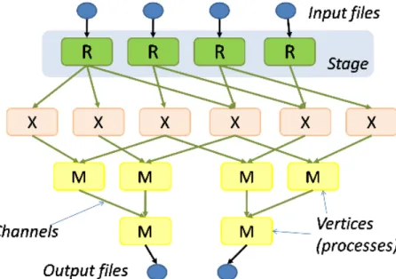
Google has developed this solution to index the Web, and provide an efficient WebCrawler. This solution is based on 3 components: GFS [215], BigTable [56] and MapReduce. The main component is GFS (Google File System). It is a virtual distributed File System (FS), which has been designed to fit efficiently to web crawl requirements (small amounts of writes, huge amounts of reads). GFS has been designed to be suitable with a highly distributed system. This system works with two different nodes: Master and Chunkservers. This solution provides a high reliability and high redundancy with at least 3 instances of the same data chunks. Then Google has provided a database system named BigTable. This DB is based on GFS, and was a data column store. All the computation is based on MapReduce. This programming model is a distributed computation model based on two functions Map and Reduce. Figure 3 presents the MR paradigm. Multiple Map functions are executed on several nodes. Results of the Map function are written in files, and the Reduce functions merge these files into other files. The original MR implementation is only suitable for batch processing; interactive processing is not suitable.

Scientists have developed an open-‐source framework named Hadoop and based on Java [95][94][107]. This strategy enables to deploy a reliable, scalable and distributed application among several computers. Instead of using Google File Systems, Scientists have developed a specific file system named HDFS (Hadoop File System). This File System enables similar functionalities than GFS. This system can store any data, without any schema requirements. To apply computation among several nodes, they also implement MapReduce. As an open source framework, this solution has massively evolved, and a plethora of extensions has been proposed and implemented. In the next section of this document, we present some of

(8)

them. An example of these extensions is presented in [142]: MongoDB can be used to store Hadoop data instead of HDFS.

2.2.

Grid computing

Grids are part of distributed systems (see Figure 2). Grids provide a set of resources by sharing and coordinating them. Grids architectures can be composed by different kinds of resources, hardware (x86, SPARC, ARM, etc.) and operating systems. All these features make Grids heterogeneous. Grids are also shared between users; each one has a specific amount of time and resources. And grids can be distributed among several locations. When a scientist has to deal with a grid system, he has to think with a possible heterogeneity of the hardware, shared resources (resources are not always available). Resources of a Grid can be distributed among countries (this implies specific network issue). An example of a grid cluster is named: GRID 5000 (France) [2]. This system is distributed among 10 sites and connected by a specific high-‐speed French network. This grid system provides to scientists a highly configurable, reconfigurable and manageable platform.

Figure 3. MapReduce execution workflow

In [3], authors describe the requirements, of grid systems: the coordination of resources with a standard protocol. They also present the most important problem with this system: fluctuant quality of service (due to the distribution and failure of resources). To manage Grid resources, a centralized system is used; and a specific protocol to enable communication among nodes. The distributiveness of the Grid system is the most complex task; it is not easy to deal with this problem. From a developer point of view, a grid system can be assimilated as a very large super computer. These super computers are virtual, because nodes are not located at the same location. Compared to a traditional super computer, network is the critical point of such systems.

(9)

Grid systems have a specific business model; it is a project-‐oriented model. The cost unit is represented by CPU hours, allocated resources and wall time. To manage these resources, GRID systems use batch submission software: PBS (Portable Batch System), Torque, SGE, etc. Grid can deal with both low hardware level and virtualized environment. Virtualized environments are used to reduce the complexity to deploy application on this system.

The next section presents an overview of cloud architectures; we present a comparison with grid because they share lot of common points. As stated in [1], the differences between both architectures are not so easy to understand.

2.3.

Clouds

In 1961, John McCarthy said, “computation may someday be organized as a public utility” [10][9]. This quote lays the first milestone for cloud computing. With this paradigm, computation is brought outside of the desktop computer. Running fewer larger clusters is cheaper than running more small clusters [53].

Multiple definitions have been proposed for cloud computing, see [4][5]. For example, cloud computing is described as a powerful service and applications, integrated and packed on the web in [4]. Cloud systems have brought a new point of view concerning requirements of IT systems [163]. Clouds are becoming one of the most used metaphors to describe Internet needs. Internet usage brings new usage and also new data structures, quantity and velocity. For example, Internet services bring new data like: text, rich text, graphs, etc [143]. Some examples of cloud services provided on Internet are storage systems like: Dropbox, box.net or Google Drive. Another example provides an email service like Gmail, or some web crawlers used on Google or Yahoo. In [174], 15 services are referenced to be used with clouds.

Cloud is considered as a cornerstone of Web 2.0. It can be used to host services, resources, applications, etc. Cloud computing refers both to the application and the hardware layers. As stated in [1], Cloud computing is a large-‐scale distributed computing driven by the economies of scale: the final price is linked with the quantity of CPU used.

Three important features compose cloud systems: processing, storage and network. To deliver resources on demand, abstract layers are used to manage cloud. Abstraction is provided by the intensive use of virtualization. With virtualization, it is possible to produce dynamically the most suitable architecture for each specific purpose. This strategy reduces the complexity for deployment. Virtualization is used on public, private and hybrid clouds. For example, on public clouds, a customer can extend his CPU resources or storage system with a credit card. This extensibility is provided by new virtual machines. The public cloud business model is based on computing and storage requirements. Resources of cloud systems are managed on demand, and they are released as soon as possible. With this strategy, Clouds systems response time is drastically reduced and users can expect a short response time (within 100ms [6]).

An example of a cloud public provider is Amazon. Amazon provides mainly two cloud services: one is dedicated for computing purposes: EC2 (Amazon Elastic compute Cloud) [199] and S3 is dedicated to storage (Amazon Simple Storage Service) [200].

(10)

In the earlier days of clouds, some companies have introduced a huge mistake on Grid and clouds. They decided to switch some of their product names from grid to cloud. This strategy led to a global mistake of the term Cloud. Moreover, as stated in Figure 2 some overlaps exist between both strategies, and a separation is not so clear. A cloud system is defined as massive, parallel, scalable and on-‐demand computing capabilities [7][10]. Differences between clouds and grids are deeply presented in [140]. Company mostly own Clouds, while grids are owned by public institutions (Universities). But cloud systems are not only restricted to companies: researchers also develop and deploy their own cloud facilities, for example using the Hadoop framework [39][44]. With this framework they are able to provide storage, elasticity and fault-‐tolerance features of a big data system. This strategy can replace their traditional data warehouse solutions [42][43]. Hadoop is also becoming the new data and computational standard for scientific needs.

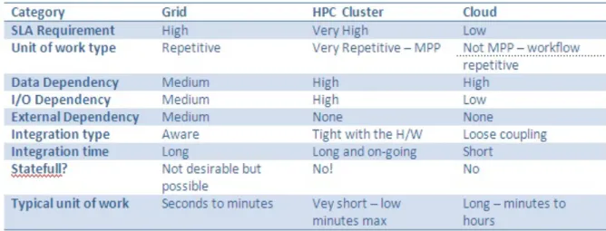
To identify the best solution between Grids and Clouds, it is necessary to identify the requirements of the target applications. In [163], the authors provide some questions to identify which solution is the most suitable: information classification, computation needed, which data will be stored and which cloud provider is the most suitable. To extend these requirements we can use different categories provided in [142] as shown in Figure 4.

Figure 4. Comparison between: Grids, HPC and cloud.

3.

Cloud infrastructures

When we want to talk about clouds, it is necessary to deal with: architecture, virtualization, management, resources on demand, services, fault-‐tolerance and analysis mechanisms. Clouds have also to be classified between public, private and hybrid. Private companies host public clouds; private clouds are hosted by a specific organization (universities, companies) and hybrid clouds use both methodology [8][10].

Private clouds are managed by a specific organization. These cloud systems have a strict complexity, a dedicated bandwidth, dedicated computation capabilities and a controlled security.

Public clouds are more traditional. Some companies sell cloud services: Amazon, Google, etc. These clouds are more traditional and suffer from different problems: service is provided over the Internet, security is related to the provider, resources are shared between a wild set of users, etc. The last cloud architecture is named hybrid and is based on multiple public

(11)

and private clouds. A virtualization layer manages services provided by these different clouds. This layer is used to create resources dynamically, in [10] these additional resources are designed to add computation or storage on demand. This virtualized layer provides the necessary resources to different cloud infrastructures. Virtualization is used as an abstraction layer between hardware, operating system and services. This strategy improves agility, flexibility and cost of a cloud system. Virtualization is used at different levels: network, storage or server. Virtualization is used to provide dynamically all the necessary resources. It brings elasticity to traditional IT systems [9]. To perform high reliability of cloud systems, these systems have been designed to be fault-‐tolerant and support an efficient load-‐balancing. Fault-‐tolerance is guaranteed by redundancy, histories and backup of data. The load-‐balancing is used to minimize job latency, avoid failover and downtime of services. When a component fails the manager will no longer send traffic to this element, this feature has been inherited from grid systems.

The next section describes different services provided by cloud systems. The second part presents storage methodologies of cloud systems. The last part presents computational methodology used with clouds.

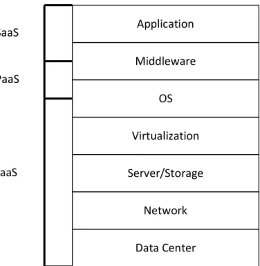
General usage of cloud systems is based on a simple paradigm named Software as a Service (SaaS). Here, the goal is to provide an application as a global service. Two other main services have to be discussed: PaaS and IaaS [146]. But cloud can also provide some other services; the literature regroups all these services under the XaaS paradigm (Everything as a Service) [85][86][146]. Some taxonomy has been proposed to present XaaS [8][146].

3.1.

XaaS

Figure 5. Cloud Layer Architecture [8]

New XaaS paradigms are proposed every day. VMware introduced an example in a recent proposal. In [119], they have introduced a DaaS (Desktop as a Service) which enables users to deploy a window for different tiny clients (desktop computer, tablet, smartphones, …). As stated in [85][86], XaaS counts at least 35 different services.

Moreover each provider (Amazon, Google, Microsoft, etc.) has produced its own taxonomy of services, thus it is not easy to provide a global taxonomy. Some examples of XaaS services are: Software as a Service (SaaS), Infrastructure as a Service (IaaS), Platform as a Service (PaaS), Communications as a Service (CaaS) or Monitoring as a Service (Maas), etc. In this document, we use the smaller taxonomy of [8]. They merge most of XaaS into three sub-‐ classes: SaaS, PaaS and IaaS. And these different classes can be stacked into layers, see Figure 5. A stricter classification is provided in [10], two classes are used: SaaS and IaaS. As

(12)

stated in Figure 7, these services can be encapsulated, IaaS can run PaaS and PaaS can run SaaS.

All these three sub-‐classes are presented in [8] and they have common points: these services are reachable through an Internet connection and through a single access point.

Software as a Service is the most common cloud service. It uses common resources and a single application instance [8]. An end-‐user can only access a single application. For example, Microsoft proposes this kind of service: Live mesh [1] (a file sharing software). GoToMeeting is another example; this application provides a cloud based meeting and collaborative tool. Now, most of Internet services are provided using SaaS: Saleforce, ConstantContact, NetSuite, etc.

Platform as a Service provides to developers an environment necessary to deploy applications. PaaS is a set of tools and services, which are able to scale with a system [8]. Google’s App Engine is an example of this service [1], a developer is able to build a scalable Web application based on the architecture of Google applications. Other PaaS providers are Force.com [212], AWS Elastic [199], Beanstalk [213] or Heroku [214].

IaaS provides dynamic hardware, software and equipment to user. This subclass of service is brought by massive use of virtualization (hardware, automation). This model is suitable for companies who do not want to buy expensive data centers. Common examples of such services are Amazon EC2 and S3, which provide dynamic storage and computation [1]. Most of IaaS providers use closed-‐source virtualization environment like: VMware or Citrix. But it is also possible to use other open source solutions like Openstack with: Linux container or KVM virtualization software.

Figure 6. A star glyph of 3V, definition of BigData [87][144]

(13)

3.2.

Storage

Storage systems have followed the evolution regarding the amount of produced data. In the earlier days of data storage, the CRUD paradigm has been defined to set requirements of traditional database systems (Create, Read, Update and Delete). A second evolution of DataBases was brought by the definition of the ACID requirements (Atomicity, Consistency, Isolation and Durability). This requirement rules the most widely used DB like RDBMS (Relational Data Base Management System). A comparison between ACID and BASE (Basically Available, Soft and Eventual Consistency) approaches is presented in Figure 8.

But regarding to the fast evolution of the data produced, the ACID paradigm is now too restrictive to be used with new data. Each year, the amount of produced data is increasing, and meta-data is used to enhance data understanding. As stated in the introduction, 3 dimensions, named 3Vs [11][142], define this fast growing: Volume, Variety and Velocity. These 3 dimensions are represented in Figure 6.

Before choosing a Data Base, it is necessary to study the structure of the target data. DB is designed to store one of thee three kinds of data: structured, unstructured and semi-structured. In the next sections, we present a classification, and some examples of DBMS, based on information in [15]. This classification is composed by: traditional RDBMS, other RDBMS (Distributed DBMS, Object-oriented, … ) and non-relational DB.

Application Middleware OS Virtualization Server/Storage Network Data Center SaaS PaaS IaaS

(14)

ACID BASE

Strong consistency Weak consistency

Isolation Availability first

Focus on “commit” Best effort

Nested transaction Approximated answers

Availability Aggressive

Conservative Simple

Difficult evolution Faster

Easier evolution

Figure 8. ACID vs Basic [201]

3.2.1.

RDBMS

RDBMS are the most popular database management systems. RDBMS means: Relational Data Base Management System. The first description of RDBMS has been produced in 1970, [20]. This DB is based on a table-‐oriented data model; the storage of data is constrained by a schema. Data records are represented as rows of table, i.e., tuples. These DBMS have some basic relational algebra operations: union, intersection, difference, selection, projection and join. On top of these DB, a language named SQL (Structured Query Language) is used. The evolution of these DB has produced a large number of DBMS: DB-‐engine [18] presents a wide DB list. This web site references different kinds of DB (NoSQL, Object-‐oriented, …). If we take a look at only RDBMS, 79 RDBMS are referenced on this website, which contains 216 references. Four RDBS are in the top 5 of this webpage: Oracle, Mysql, Sql Server and PostgreSQL.

MySQL is an open source RDBMS. It is one of the most famous RDBMS because it has been massively used with web applications. This DB has been developed to answer to direct requirements of users. It supports multi-‐threading and multi-‐user accesses. This DB has been created in 1995, and the implementation is done in C and C++. It is possible to access to this DB using several languages: Ada, C, C++, C#, D, … A distributed version of this DB exists and was named MySQL cluster. Replication is also provided.

Oracle DB is a database marketed by the Oracle Corporation. It is a closed-‐source DB, which can be deployed on any OS. This DB has been developed in 1980, using C and C++. It is possible to use it with any programing language. This DB supports partitions and replication methods. This DB supports also multiple users at the same time.

SQL Server is a commercial product delivered by Microsoft. It has been developed since 1989. It is a commercial DB, developed in C++. It can only run on a Windows instance. It is possible to use this database with .NET language or Java. Data can be distributed across several files and replication depends on which version of SQL Server is running. Multiple users can use this DB concurrently.

(15)

3.2.2.

Object Oriented DataBase

An object database is a database management system in which information is represented in the form of objects as used in object-‐oriented programming. Object databases are different from relational databases, which are table-‐oriented.

Object-‐oriented database management systems (OODBMSs) combine database capabilities with object-‐oriented programming language capabilities. OODBMSs allow object-‐oriented programmers to develop the product, store them as objects, and replicate or modify existing objects to make new objects within the OODBMS. Because the database is integrated with the programming language, the programmer can maintain consistency within one environment, in that both the OODBMS and the programming language will use the same model of representation. Relational DBMS projects, by way of contrast, maintain a clearer division between the database model and the application.

Express Data Manager™ (EDM) (see [225] for more information) from Jotne EPM Technology is an object-‐oriented database that is well suited to handle both structured and unstructured FEM and DEM data. The reason for this is that ISO has standardized an object oriented schema for storing and exchange of FEM and CFD data, ISO 10303-‐209,Multidisciplinary analysis and design (AP209). The schema is written in the modelling language EXPRESS (ISO 10303-‐11, see white paper on [226]). EDM is designed to handle EXPRESS objects and is by that a good choice database system for standards based and, thus, interoperable FEM, DEM and CFD data.

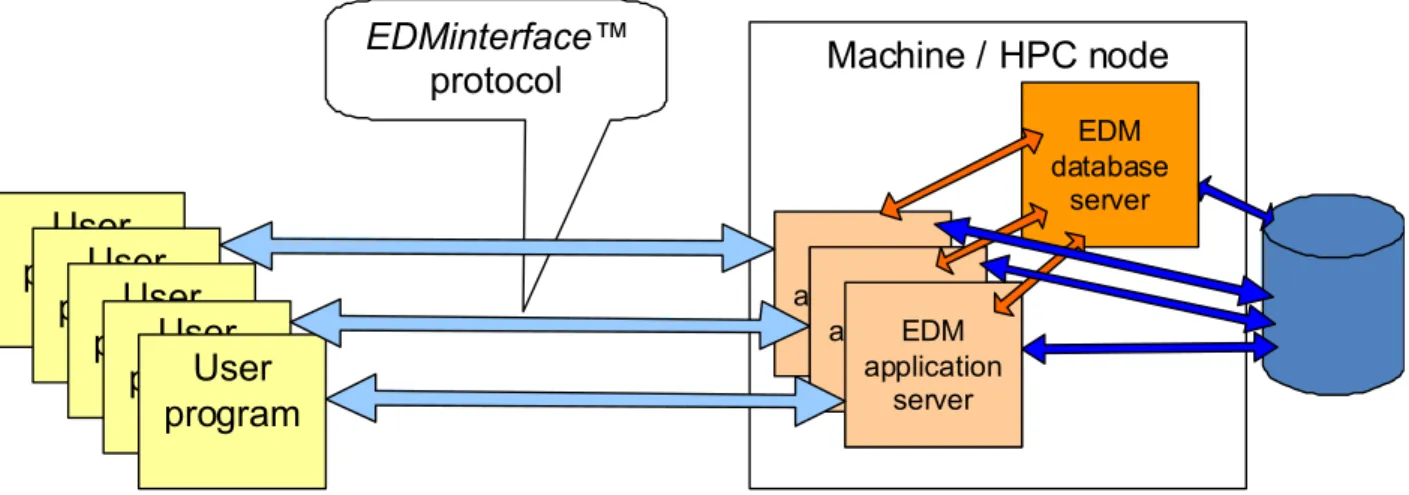
EDM is a database system that is well suited for deployment on HPC clusters; see Figure 9, below. The EDM database server, EDMserver™ consists of one database server process and several application server processes, as indicated on the right hand side of the sketch below. The database server performs initialization functions, like compile EXPRESS schemas, create users, repositories, models (datasets) etc., and synchronisation functions between EDM application servers. It is the EDM application servers that execute the database queries, and these EDM application servers can be deployed on several machines concurrently.

Figure 9: EXPRESS Data Manager (EDM) in the context of a HPC cluster Machine / HPC node User program EDM application server EDM application server EDM application server EDM application server EDM application server User programUser programUser programUser program EDMinterface™ protocol EDM database server

(16)

The communication between the EDM application servers and the database server is implemented by messages over TCP/IP. By that it is easy to distribute the application servers on many machines. The TCP/IP approach is better suited for HPC clusters than communication solutions using, for example, shared memory messages, semaphores etc. . An EDM database can have many independent datasets, in EDM terminology called models. Each EDM application server may update one data model; therefore, this architecture allows parallel updates of the database. If the scenario requires a database that consists of one huge dataset, all EDM application servers may read this model concurrently. Queries may be split into subqueries, and each subquery may be assigned to one EDM application server. The result is an implementation of the Hadoop Map/Reduce pattern.

The EDM database is an object oriented database system where each object has a "database global" object id; the object id is a 64 bits integer. The uppermost part of the object id is the model number of the model that the object belongs to. The lowermost part of the object id is the object number within the model. By this great object address space it is only disk size on the database server that limits the size of the database.

These characteristics make the EDM database system a good starting point for implementing efficient FEM/DEM queries on a HPC cluster.

OoDBMS (Object oriented DBMS) was developed to improve storage applications. Objects produced by software are directly stored in OODBMS. Schema of data is provided by the applications. Some existing DBs have evolved to support this new paradigm, and others have been developed. Some examples of these DB are: Cache, DB4o, Versant Object Database or PostgresSQL.

PostgresSQL is developed since 1989. It was developed in C and can run on any operating system. This DB can be used with several programming languages: .NET, C, C++, Java. This DB is mostly Object-‐oriented, and it does not support the partitioning of data. Replication is performed using a traditional master-‐slave solution. Multiple users can use this DB.

A deeper comparison between RDBMS and OODBMS is provided in [231]. Data of OODBMS contains both execution part and information. In a RDBMS, only data are stored into a two dimensional view (table). In an OODBMS, data are stored into structured objects. Authors of [231] say that OODBMS must be used for complex data and/or complex data relationship. OODBMS are not recommended when only a few join operations are necessary and when there is large volume of simple transactional data. This document also provide information regarding to advantages and disadvantages of RDBMS compared to OODBMS. These information are quite useful to determine which solution is the most suitable regarding to data and operation over data.

3.2.3.

Other RDBMS

To be more suitable with new data requirements, RDBMS have also evolved. DBs have evolved to support multiple instance of the DB.

To increase performance of DB, solutions have been proposed to use multiple nodes. Thus two solutions arise: the first one uses distributive properties (like the solution powered by Google: BigTable), the second one uses parallel databases. To be able to deal with BigData, it is necessary to use distributed DBMS. In 2006, BigTable has been presented in [56], it is a

(17)

distributed file system management, which can be used to store data in a distributed way. These parallel DBs are designed to run on multiple nodes, with multiple CPU and using parallel storage systems.

3.2.4.

NoSQL

NoSQL describes DataBase, which do not only deal with SQL. A clear definition of NoSQL does not exist, and the points of view can diverge. An example is presented in [16]; NoSQL is described as a distributed DB without any fixed schema. Sometime, NoSQL refer to a non-‐ relational system. Another definition of NoSQL DB refers to a structured DB. A common property with all NoSQL definitions is Web 2.0, huge amount of data and huge amount of users.

This DB has been introduced in 1998 and has reached a growing interest in 2009 [16]. These DBs do not use ACID schema, thus they are able to achieve higher performance and higher availability, compared to traditional RDBMS. Store and retrieve mechanisms are also different.

As stated in [15][16], NoSQL DBs can be classified into different types: Key-‐Value, Document, Column, and Graph. Some other classifications are available, see [17]. In this document, we use the most common classification: Key-‐Value, Document, Column, and Graph. This classification of DBs is based on [14][18].

3.2.4.1.

Key-‐Values

The Key-‐Value strategy allows the application developer to store data with a schema-‐less approach. Two fields represent data: a key and a value. This strategy allows storing data using an arbitrary index based on a key. Both fields of this DB depend on the applications [88]. This mechanism can be found in several DB: Redis [24], CouchDB [88], Cassandra [88]. A more complete list of Key-‐Value databases is presented in [17][202].

3.2.4.2.

Document

Document DBs store data with named documents. The engine is used to manipulate these documents and improve storing, retrieving and managing. Using a document storage approach allows to deal with semi-‐structured data. Access of data is done using a unique key for each document. This methodology have been implemented into: MongoDB [24], CouchDB [24], Riack [24], etc.

3.2.4.3.

Column DB

In a column DB, data is stored in tables. Each table is structured with a column schema. This strategy serializes all data onto columns. This strategy has been used in several DBs: BigTable [17], Hbase [24] and Cassandra [24].

(18)

3.2.4.4.

Graph

The last kind of NoSQL DB is named Graph DB. This DB uses a graph structure to store data, composed by: nodes and edges. With this strategy, every element contains direct access to adjacent elements. With this method, no indexes are necessary. Examples of graph DB are: Neo4j [24], FlockDB [17], OrientedDB [17], Pegassus [31] or Pregel[30].

3.2.5.

The case for VELaSSCo

In this section, we will propose a summary of VELaSSCo needs concerning the storage system. Data of this project will be produced by two specific simulations: FEM and DEM. For Discrete Element Methods, particles and contacts can be created and lost during the whole simulation. For both solutions, a solver produces relative small files, which contain the different time steps of a simulation (See D1.3, section 2.5, page 18). These files will be structured regarding to a specific format. The amount of data produced by these solvers depends on the number of generated time steps, it is also depends on the number of nodes/Elements (FEM) or particles (DEM) involved in the simulation. The velocity of produced data vary regarding to the simulation engine.

As the data already exists in distributed files at day 0 of the project, it is necessary to find a distributed system, which enables to inject the data based on a key value or document oriented approach into the DB (key = analysis_name + time_step + result_info + partition_info, value = result_values). With this methodology, the complexity of integration is drastically reduced. Data storage needs to be directly reachable by a HPC facility. If the DB system is distributed, thus the location of information has to be transparent.

Figure 10. Expected revenue of different DBMS [221].

3.3.

Computation

Computational models of DBMS can be divided into two different strategies: complex and simple queries.

(19)

Complex queries apply complex operations (join, selection, projection, etc.) on data. A simple query uses a simple model: extract data from the dataset (without any result enhancement). Complex queries can be expressed by simpler queries.

From these two models, some specific query languages have been proposed. In this paper we present only two of the most used models: SQL and MapReduce. SQL can express complex and simple queries, while MR is used to express simple queries (some extensions of MR have been proposed to improve this simple query model).

This section is dedicated to compare these strategies. We present how computational models work, describe when these methods have to be used, and which drawbacks arise from these models.

3.3.1.

SQL

Most of traditional RDBMS systems use complex queries to manage their data. SQL is a normalized language used to exploit DBMSs. This language has been built on top of CRUD (Create, read, update and delete). SQL also supports more complex queries like: joins, transactions, etc. This language has been developed to run one-‐time queries. Most common SQL systems do not provide suitable tool to run long queries, and the results of these executions are sent to the users at the end of the computation.

Unfortunately, the fast growth of datasets introduces new requirements for data computations. An answer for these requirements has been presented in [74]. Authors proposed a Data Stream Management System (DSMS), as an alternative to the traditional DBMS systems. This project deals with three important features: the first one concerns streamed data where data is sent at runtime, and it is not necessary to wait the end of a computation. The second feature concerns load variability (system deals with variability of queries) and the last part concerns the management of resources. To perform these continuous queries, authors have introduced a new language named CQL (Continuous Queries Language). This modern paradigm brings new challenges: necessity to provide suitable stream structures, and traditional declarative queries need to be translated into specific continuous jobs.

A DSMS needs specific features; it is necessary to deal with coarse data (sometime accurate results are not possible and degraded results have to be sent). In [74], authors provide a centralized monitor and manager of queries. With this methodology, system workload is always under control. This project is unfortunately no longer maintained, and has been stopped in January 2006.

3.3.2.

MapReduce

The second computational methodology is for simple computational tasks. The most used model is MapReduce. This methodology is composed by two functions: Map and Reduce. Map function is used to filter and sort the data, while the Reduce function is used to aggregate and summarize data produced by Maps. This methodology is described in several papers: [19] [35][58]. In the original paper, MapReduce was implemented using the Sawzall functional language [35]. Google has popularized this methodology with one paper: [89]. The Hadoop framework provides an open-‐source implementation of MapReduce [49].

(20)

MapReduce has massively been used for words search and count, but this simple computational model is not suitable for complex queries, and expressing more complex computations requires drastic code modifications. In the scientific community (Machine Learning for example), MR has some difficulties to express iterative algorithms, thus it is necessary to find new solutions. Problems that cannot handle efficiently with MapReduce are presented in [25].

3.3.3.

Procedural approach

The EDMopenSimDM™ system (see: [227] or [228]) offers AP209 engineering queries to the end user. Examples of AP209 queries are Model Query, Node Query, Element Query, Element Property Query, Displacement Query and Stress and Strain Query.

These AP209 queries are built upon the EDM C++ Express API. This is a generated C++ interface to the EDM database objects of AP209. Each EXPRESS entity (object class) is mapped to a corresponding C++ class. The generated C++ classes have put and get methods for all attributes. The EDM C++ EXPRESS API is an extension to the EDMinterface™ API, which is shown in Figure 9, above. See also the EDMinterface™ chapter in EDMassist in [229].

In the AP209 engineering queries each query is implemented along the following pattern:

1. The objects to be queried are either all of one specific class, a range of objects, objects with specific ids or objects that satisfy pattern matching search criteria. 2. For each object of interest, the database object is located by different access

methods dependent on the search criteria. If all objects of one specific class shall be visited, the query traverses the list of all objects of that class. If specific objects ids are the search criteria, attribute hash tables are used.

3. When an object of interest is found, the C++ get methods are used to retrieve information about the object and all other relevant objects for the query.

The AP209 engineering queries developed for the EDMopenSimDM™ system are a good starting point for developing visualization queries for FEM/DEM objects.

3.3.4.

The case for VELaSSCo

To identify the most suitable strategy for the VELaSSCo platform, it is necessary to identify its needs. Discussions with the partners highlight some requirements: an efficient computational model, a distributed computational model, a simple interface to access data and a computational model suitable for batch and online queries.

To store data, the most common habit is based on SQL storage; developers have been formed to use SQL engine. Thus switching to a new paradigm like MapReduce is not a simple task. To deal with Big Data, it is necessary to evaluate the performance of both model, see [19]. The rest of this section describes some differences between these two models regarding to the VELaSSCo project.

(21)

EDM, on the other hand, is a strongly object oriented DB, in which associations between objects are very important, are another key value in the system. The format followed is the one defined in AP209. As the input data does not have this information, it should be created when the simulation data is injected into the system, like defining the mesh-‐groups, identify the distributed parts that belong together, group the results of the same analysis and time-‐ step, etc.

The first difference is on data structures: MR allows arbitrary data formats, while DBMS requires well-‐defined data formats. MR and parallel DB share some common elements, but some noticeable differences appear in both systems. This missing schema can produce data corruption, while a strict schema makes SQL DBs less flexible.

Another difference between DBMS and MapReduce resides in the indexing of data. The index of DBMS is based on hash or B-‐tree, while MR framework does not provide a built-‐in index. MR programming model needs a higher language to be more user-‐friendly, and MR can be compared to a low-‐level language like assembler. Hive, Pig, [42][73][123] have emerged to propose this higher language, and in [158] other SQL abstractions are presented. These solutions bring SQL abstractions on top of MR, thus it becomes less difficult to interact with the MR computational model. SQL queries are translated into a set of MR jobs. Hive, [46], brings also an improved file storage system [122]. This storage strategy (ORCFile) compresses data and brings good compression results (78% smaller than raw information). Outputting results from RDBMS and cloud solution is also different (in their traditional methodology). With the MR computation, it is necessary to create manual data filter. In the case of RDBMS, data is already filtered. This issue is also similar regarding to intermediary steps, RDBMS uses raw data, while MR writes intermediary files.

Finally, MR provides a native sophisticated fault-‐tolerance model compared to RDBMS; this advantage comes from the built-‐in high redundancy of data [21]. From these different key points, [19] have proposed several benchmarks based on the original MR task: Grep Task, and four HTML specific tasks (selection, aggregation, join, UDF aggregation (user defining function)). Then the authors make a comparison based on user-‐level aspects. This benchmark shows that in most cases, parallel DB are an order of magnitude faster than MR. But MR is more user-‐friendly, and deploying this system is easier than a parallel DB. Extensibility is also in favor of MR; DBMS are not well suited for such tasks. Some of the discussed VELaSSCo queries, which requires the processing of the distributed information and the fusion of partial results, which also may require some distribution-‐fusion calculation iterations, can be harder to implement in EDM than in map-‐reduce.

In the specific case of VELaSSCo, a hybrid computational model can be more suitable. It is important to provide an extensible approach which can answer to well define requirements and which can be extended to future needs. One of the requirements for the VELaSSCo platform is to support special particle shapes, or cluster of particles, which can be implemented on other systems, but requires an extension of the AP209 standard so that the EDM systems support them too. In the meantime may be they can be treated as mesh of particles, for the cluster, so that a 'mesh of particle clusters' would be represented as a 'mesh of mesh of particles' in EDM/AP209.

(22)

4.

Best practices

With a major evolution of usage, cloud systems need some improvements, evolutions. These modifications have to be focused on cpu usage, long run time computation, etc.

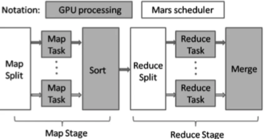
To manage this new amount of data and computation, industries and scientists use a cloud approach to perform both computation and storage. Cloud systems have to be scalable, see [191]. Three scale strategies exist: scale out, scale up and scale side-‐by-‐side. Scale out is used to refer to the increase of number of nodes (machines). Scale up increases the capacity of a system. And the last methodology is used to deploy a temporary system, used for test and development. Regarding to actual state-‐of-‐the-‐art, a large variety of cloud architectures are based on Hadoop; see [34][40][42][50][80][177]. Computations presented in most cloud systems use the MR methodology.

In this section, we present some best practices used to improve cloud architectures. Our interest is focused on virtualization, storage and computations improvements. The last part presents software stacks.

4.1.

Hardware

IT systems used for Big Data have multiple tradeoffs: data storage, network resources, computation capabilities and energy efficiency, see [203]. This section presents optimizations provided by scientists at different hardware levels.

4.1.1.

Storage

Computer hardware is composed of two different storage systems: main memory and secondary storage systems. Both solutions have their own advantages and drawbacks. The main memory (RAM) is mostly used to store cached data or current used data. This system