Visual Analysis for Extremely Large Scale Scientific Computing

(1)

Visual

Analysis

for

Extremely

Large

‐

Scale

Scientific

Computing

D2.2

–

Specification

of

Big

Data

Architecture

Version 3.0

Deliverable Information

Grant Agreement no 619439

Web Site http://www.velassco.eu/

Related WP & Task: WP 2, D2.2, T2.2

Due date September 30, 2014

Dissemination Level

Nature

Author/s Ivan Martinez, Tomas Pariente,

Contributors Alvaro Janda, Andreas Dietrich, Benoit Lange, Olav Liestol, Miguel A. Pasenau de Riera, Jochen Jaenisch

(2)

Approvals

Name Institution Date OK

Author Ivan Martinez

Tomas Pariente

ATOS

ATOS 30/09/2013

Task Leader Ivan Martinez ATOS

WP Leader Toàn Nguyên INRIA

Coordinator Change Log

Version Description of Change

Version 0.1 First draft version of the document

Version 0.2 Draft including Olav and Benoit contributions

Version 0.3 Draft including Andreas contribution for visualization chapter Version 1.0 Semi‐final version including Alvaro contribution in HPC

section and DEM data. Version 2.0

Release version including contributions for visualization engines section and FEM data of Miguel A. Pasenau and contributions in general section of ATOS.

Version 3.0 Final Releases including review updates

(3)

Table

of

1. Introduction

Based on the literature surveyed in task T2.1, this document specifies in the scope of task T2.2 the general system architecture from a big data perspective.

A main focus in the distributed development of a system is the specification of the architecture and the integration processes to support the integration of several components into a single system. It is also relevant to propose a modular configuration of the system to fit with the different use cases defined in the project.

Architecture and integration standards are separated into different aspects of development. The architecture describes the structure of a system while the integration focuses on the process of fulfilling this architecture. The architectural standards focus on the correlation of all services and components and the “integration” of external legacy systems into the VELaSSCo system while the integration aspects focus on the set of tools, procedure and interfaces to support the communication and computation of VELaSSCo. Therefore the ICT architectural and integration aspects focuses on two main processes:

 the definition of an integrated architecture supporting the conceptual structure of the VELaSSCo system and,

 the set of processes and tools to support the distributed development and further combination into one system.

In the case of VELaSSCo the architecture proposed should be able capable of handling efficiently the various data produced by the software tools, taking into account the various execution overheads of each particular processing tool, while ensuring a consistent and effective use of up‐to‐date data by the user, as they are made available.

Therefore, this document reports on the specification of the big data architecture most suitable for VELaSSCo simulation data environment, taking into account the deliverable D2.1 regarding State‐of‐the‐Art of Big Data approaches, such as the Lambda architecture, which finally has been selected to instantiate the VELaSSCo Architecture.

(5)

2. Concepts

of

VELaSSCo

Architecture

The goal of the current section is to introduce the core concept of VELaSSCo Architecture which is the Lambda Architecture Approach next to some relevant concepts associated to VELaSSCo project from a conceptual and technical perspective.

The Architecture of VELaSSCo platform will be based on Lambda Architecture (LA) proposed by Marz [1]. According Marz “LA aims to satisfy the needs for a robust system that is fault‐

tolerant, both against hardware failures and human mistakes, being able to serve a wide

range of workloads and use cases, and in which low‐latency reads and updates are required.

The resulting system should be linearly scalable, and it should scale out rather than up”.

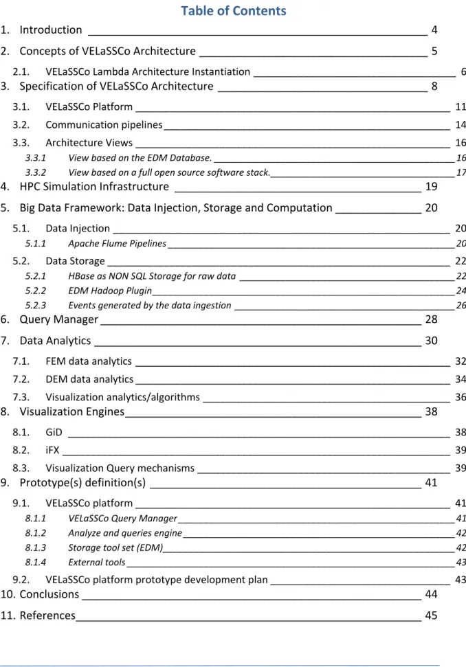
Figure 1 shows the LA from a high‐level perspective:

Figure 1: Overview of the Lambda Architecture [1].

Essentially, the Lambda Architecture comprises the following components, processes, and responsibilities:

1. Data Sources: Are the sources of all data to be made available to the solution. The Big Data solution must have the ability to capture any data source. To this solution usually have connectors or adapters to receive, capture data already stored in external databases, text files or applications or circulating information generated by sensors, social networks, mobile devices, etc. In this way the data is they make available the following layers of either architecture for storage and subsequent processing (batch layer) or real time processing (speed layer).

2. Batch layer: This layer is responsible for storing the data in what is called Master Dataset and pre‐processing of information for generating pre‐computed views.

(6)

Hadoop's HDFS is typically used to store the master dataset and perform the computation of the batch views using MapReduce.

3. Serving layer: This layer must be able to combine the results of the pre‐processed data in Batch processing layer with the data exposed through the Speed layer. It must also be able to index and display the data so that they can be consulted.

4. Speed layer: Due to the high degree of latency batch processing layer, and since there will generally be some data need to be exposed to a faster mode, a layer of processing real‐time information is required. To this layer is called Speed layer and is responsible for processing real‐time data stream that needs to be exposed immediately. As the data stream is accessible information is automatically analyzed and pre‐computed, generating views that expose these data for consultation.

Precisely because the functionality is intended to cover, the data exposed through the Speed layer are transient and are available only temporarily; while not precisely be through batch processing layer.

5. Queries: Lambda architecture answered any kind of incoming query by merging results from batch views and real‐time views.

2.1.VELaSSCo Lambda Architecture Instantiation

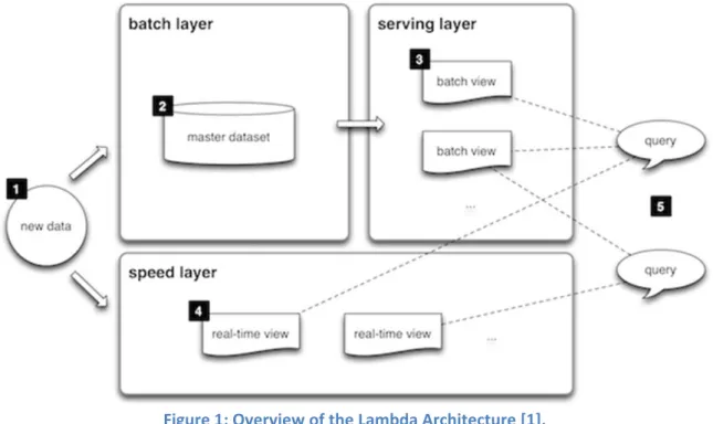
Subsequently, the Lambda architecture instantiation proposed for VELaSSCo from a service point of view is presented in Figure 2:

Figure 2: VELaSSCo LA instantiation

To handle, store, and visualize the amount of data that will be generated from the future engineering simulations, it is imperative to use large scale distributed computing

(7)

infrastructure such as used in Big Data infrastructure. The architecture diagram of the big data infrastructure in the context of engineering application is shown in the Figure 2. It primarily consists of three layers: batch, speed, and service layers.

The roles and functions of these layers are summarized as follows:

1. The engineering data from the simulation is constantly sent to the HPC clusters with the help of the petabyte sized data interface, thus creating a constant growing master dataset. With this constantly growing dataset, the batch layer starts.

2. The batch layer pre‐computes query functions (based on the domain knowledge) on subsets of data of the master dataset, and then store the partial results in flat files, called batch views. The views are created in order to achieve low response time in implementing a send result approach (for more details see the visualization engines section).

3. In order to correctly, and quickly send the target files based on the users queries, these files are indexed by the database that is specialized for engineering simulations. The service layer holds the database.

4. As soon as the request for the visualization enters the service layer, the database fetches appropriate computed partial results available through the indexing mechanisms. These results are either sent to the clients, where the GPUs available on the client side can make visualizations out of the sent results by leveraging the newest OpenGL features , or streamed via the rendering nodes of the HPC clusters to the potential clients

5. While the batch layer performs its pre‐computation, if any new data arrives, then they are sent to the speed layer. The speed layer runs incremental algorithms and helps in visualizing only the real‐time (recent) data.

6. Visualization queries are resolved by getting results from both the speed layer and batch layer.

(8)

3. Specification

of

VELaSSCo

Architecture

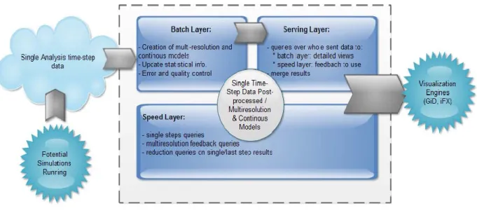
This section presents specifications of the architecture for the VELaSSCo platform. This platform is designed to support engineering data used and produced by simulations. As stated in the literature, data produce by scientific communities grows in an exponential way, and at the same time, the analysis algorithms are more and more complex and take more time. Thus to enable more efficient computations, it is necessary to use large computing infrastructures instead of a single node. Conceptually, most simulations produce raw data, composed by lists of integers, floats and doubles. An effort is required to manage this information and produce useful visualizations. Big data frameworks include a building block in charge of data analytics conceived as a sophisticated process that extracts pieces of information from the data, and apply specific computations to extract the desired features. A global overview of the platform is presented in Figure 3.

Figure 3.VELaSSCo infrastructure.

With the VELaSSCo project, our consortium tries to propose an answer to different requirements of scientific visualization and big data production.

The first requirement of the architecture is to be effective on most scientific hardware. As stated in Deliverable 2.1, the traditional architecture of Big Data is composed by some commodity nodes (with simple hardware capabilities, low speed network (typical network connection) and local efficient storage). While for scientific usage, compute facilities are composed by a small set of high performance nodes, managed by a resource scheduler. In a commodity center, the number of nodes is the most important aspect as BigData performance scales linearly with the number of nodes, while in HPC centres the focus lies in a high speed network which communicates several thousand compute nodes but with a 'centralized' viewed storage, i.e. with almost no local storage which is scarcely used. The targeted architecture depends on the available infrastructures, thus it is necessary to find an

(9)

efficient solution to make compatible a BigData framework on a HPC cluster. The software stack used for this project has also to support most of the requirements of big data. That means: how to dispatch efficiently the computations among nodes, how to use the advanced features of modern and old CPUs, and how to deal with the fault tolerance and failovers. Small changes in the HPC infrastructure may be needed for a successful deployment for an efficient adapted BiGData solution, such as the incorporation and usage of local storage on some of the computation nodes of an HPC cluster. The compute intensive simulations running on an HPC cluster will send the data to our solution, deployed in the same cluster, and the user can access and analyze this data in an efficient way through a specific smart and user‐friendly interface. The solution needed for this project may also be transportable to a cloud oriented infrastructure: the users will be unaware on how and where the computation is performed, but accessible through the same user‐friendly interface.

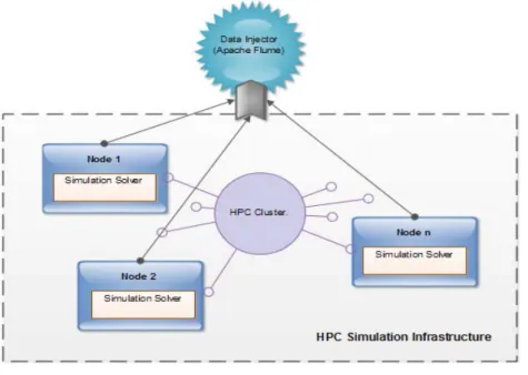
For the second (Big Data) requirements, our architecture has to deal with data location and storage, see Figure 4. In this project, a specific HPC cluster will produce simulation data. To be able to perform large simulations, engineers decomposes the problem data into as many sub‐domains, also called partitions, as compute nodes are used to solve the simulation. The each compute node outputs the results of the simulation for its sub‐domain. For this purpose, Flume seems to be the most suitable tool to ingest the several partial results into the BiGData system. With this strategy, maybe it is necessary to use an aggregating solution to inject data into the VELaSSCo platform. But the BigData framework also splits a data set among several data‐nodes for efficiency and fault‐tolerance purposes. May be is it possible to take profit of the smart partition the simulation engineer has done and use it to distribute the simulation results among the data‐nodes. In a high performance simulation environment, each compute node deals with a sub‐domain of the dataset, and produces its own result file (one for each time‐step). Flume grabs these files from the compute nodes and stores them into the VELaSSCo platform using agents. Flume can be in charge of the aggregation of the same time‐step and to store it. For the storage part, we plan to use an existing layer of the Hadoop distribution. Hadoop provides an abstract class for file system storage; this enables a high extensibility of the storage system. The Flume agents will put the data into the storage system through this abstract file layer. Flume supports this Hadoop storage layer and is able to use existing components like Hbase to sort efficiently the data. The data can be written into native format (tabular), with an efficient hash table (using Hbase). With none tabular data, it is possible to use directly the HDFS file system in RAW format.

(10)

Figure 4: HPC Simulation Infrastructure

The third requirement concerns the query engine layer. The visualization client of the user will communicate with this layer to analyze the simulation data and get the results of these analyses for visualization. A user request, for instance display the average damage of a certain surface of the model, will issue one or more queries to the 'query engine layer'. Within this layer, a user query is analyzed and, depending on the work‐load it represents, splitted into different sub‐queries which require the collaboration of the Batch, Real Time (RT) and Analytics modules. At the end the sub‐queries access the data layer, where a “search“ engine gathers information from the storage using a specific pipeline. Information is then delivered to the user into large pieces of data (Chunk). It is the most traditional layer used by database systems.

Heavy queries are queued in the Batch module and the same query is sent to the Analytics+RealTime modules but on a simplified model of the simulation data in order to fulfill the third requirement: ensure that the user is able to interact with the data. For the real time queries, a specific engine is in charge of fast streaming of data, and requires a dedicated format. To be able to reach this capability, pre‐computed data and efficient data structures need to be stored into the data layer. The analytics module is in charge of all calculations and analysis tools of the query engine, example of these analytics tools are:

 Computation of multi‐resolution model,

 The temporal and spatial statistical averaging of the results on particle simulations  Extraction of features such as skins of volume data, streamline and iso‐surface

calculations, etc.

For the final requirement, the architecture has to support extensibility. Obviously, all components needed to fulfill the other requirements are not yet developed; an extensible platform will help us to integrate and manage them. To deal efficiently with BigData

(11)

requirements and extensibility, the VELaSSCo platform uses Hadoop. With its high extensibility it is possible to extend Hadoop with for example the support of the EDM DB on the data layer. Hadoop extensibility also allows deploying this ecosystem on top of any IT system. With this extensibility, it is also possible to deploy components regarding to the data set. For example, it possible to deploy a VELaSSCo platform to only stores none tabular data, thus Hadoop plugin will only be related to such kind of data.

3.1.VELaSSCo Platform

The VELaSSCo platform is the core block in the VELaSSCo architecture described in the section 3. From a layered perspective, the platform is composed of three layers:

 The first layer, I/O or Data layer is composed by a gathering tool (Flume) next to a monitoring tool to know the status of different process. The data query layer is connected to the I/O interface with the Hadoop ecosystem. Example of this interfaces are Hive Storm, Hbase, etc.

 The second layer, query engine layer, concerns the analytics, batch and real time modules of the platform. This layer is managed by YARN [5]. It is the specific resource manager for Hadoop 2.x. With this software Hadoop supports any kind of computational model. This strategy enables to support more complex computational models, and MapReduce is not anymore the only option. Thus other tools like multi‐ resolution, convertors, etc. are feasible.

 Finally, the storage component, concerns the storage system of the platform. With Hadoop extensibility, most existing storage systems are supported. VELaSSCo will not only work with Hadoop storage system but also provide new storage facilities with the EDM DB. This strategy is similar to the HadoopDB approach.

(12)

A logical view of the platform disclosing the different layers from which the platform is composed is depicted in Figure 6.

There will be two layers:

 Data Layer: which is responsible to store, access and translate the data and will answer the data queries coming from the "Query Engine Layer" and, eventually, when data is ingested in the platform, it may generate simplification queries, to create coarser views of the simulation data (corresponds to the I/O and Storage layer of Figure 5);

 Query Engine Layer: which is the responsible for receiving the user requests (VELaSSCo queries) from the visualization client, process them, generating data queries to the Data Layer, processing the returned results, eventually merging them, and format this results in a gpu‐friendly way for the visualization client (corresponds to the Yarn layer of Figure 5).

In addition to these two layers, two libraries/modules will allow the connection between the platform and the final user:

 Data Ingestion library: which will provide a mechanism to ingest data from the computer engineering simulation solvers to the VELaSSCo platform. After establishing the communication with the Data Layer, including user validation, the ingestion module will send the data to the Hadoop Abstract File System. The Data Layer will store the data in P4 / GiD format if the HDFS is used as storage or translate the data to STEP/AP209 when using the EDM‐plugin and EDM‐DB system.

 Platform Access library: will communicate the visualization client and translate user requests into VELaSSCo queries, receive the results and show them to the user. The module will also generate VELaSSCo queries automatically, for instance when the user just navigates through the simulation model, or to ensure interactivity it will handle coarser models and issue full‐detailed queries when the user zoom on parts of the simulation model.

(13)

Figure 6. Layers and modules involved in the platform Inside the Query Engine layer following modules are to be developed:

 QueryManager: responsible for managing the VELaSSCo queries, evaluate their costs and issue Fast queries and, eventually, Batch queries. If a query is too expensive, i.e. it will take too much time to evaluate, this module will launch both, a simplified version of the query (using a simplified version of the simulation data) to provide feed‐back to the visualization client and a full detailed batch query, which will access the full‐detailed simulation data. The queryManager will also synchronize and control the visualization parameters and issue visualization queries to the Real Time module, like the 'traveling' through the model for an interactive navigation.

 Analytics module: responsible to perform data analytics over the stored simulation results. It will also provide a cost estimation of the data analytic query to help the Query Manager evaluate in which mode is the analytics to be evaluated: in Speed mode or in Batch mode. This module will also generate coarser versions of the simulation data in order to provide fast feedback to the user and the Discrete to continuum transformation needed by the DEM simulation data.

 Batch module: responsible to perform heavy data analytics and to provide feedback on the progress of the query.

 Real Time module: responsible of providing feed‐back to the user whether in full detail (for instance of detailed views of navigation through the simulation model),

(14)

simplified version (for heavy queries and when the coarse view is present) or progress indicator of the batch queries being executed; also for preparing the data for a fast visualization in the visualization client.

As already explained the communication between the Data Ingestion library (glued to the simulation program) and the Data Layer will be done using Apache Flume, and the communication between the visualization client + platform access library and the Query Engine Layer will be done using Apache's Thrift.

As for the communications between modules, as they are modules integrated inside a Hadoop framework, it will follow Hadoop recommendations just adapted for the FEM/DEM analytics needs.

The data to be passed between components will be reduced to basic types (string, integers, long integers (int64, doubles) or basic type lists/arrays.

The GPU‐friendly format used to communicate the results of the query between the Real Time module and the visualization client will be detailed in a following annex, but can be viewed as a byte‐stream or a byte‐array

3.2.Communication pipelines

A detail overview of the platform is presented in Figure 7.

(15)

This schema gives an overview of all the communication pipelines. It presents a deeper representation of the infrastructure with the communication data flow. Blue arrows represent the data transfers, while green arrows represent queries.

In the engine layer (Yarn), some examples of plug‐ins are presented; each module (batch, RT and analytics) can be extended with other applications. This strategy allows bringing new capabilities to the platform in the future. In Figure 7, two execution queries are presented: on the server side (black octagons) and on the user side (purple circles).

The first pipeline is representative of a storage plan. For this purpose, only compute nodes are involved in the process. In (1), data is produced by different nodes using their simulation engine. Then, Flume agents aggregate this data and write it into Hadoop through the abstract file system. This abstract file system then writes data into the appropriate file storage system, for example on a standard storage system (HDFS, Lustre … 3a) or using EDM, with a conversion from a file format to EDM/Step AP209 (3b).

For the second workload, a query based on visualization is performed, and transmitted to the query layer (2) using Thrift. The user account is validated and the query is transformed into an analytic query (for example mesh simplification) (query 4a). The analytics module gathers information from the file system and processes it. Eventually a quick simplification is performed and the produced data is stored (and obviously dispatched to the correct storage system) (5 and 6). Then the produced data is sent to the real time and transmits the result data, with Thrift, in a suitable format for the visualization engine and finally, the rendering is performed by the viewer (8 and 9). Information concerning the query and progress is sent to the monitoring tool (4b) which also monitors availability and resources statistics of the platform

This example shows how storage and queries are processed in the platform. An important point of this architecture is the support for extensibility. All necessary plug‐ins can be deployed, regarding which data will be stored and which computations are performed. To avoid multiple connections and multiple protocols, the query related components are in charge of communication between the user and all compute models. With this strategy users can perform Hive, Hbase or any kind of other query in a transparent manner.

The generic base of existing software developed for the Hadoop ecosystem provides multiple options and opportunities to adapt the VELaSSCo platform to a large number of applications and user requirements.

To validate some of these components, we performed an experimentation based on a new tool called “GDF” (Generic Deployment tool For Hadoop)[6]. It allows the deployment of a set of Hadoop components, based on a description of user requirements. This strategy allows supporting any IT system. Each required tool is then deployed over the user specific IT system: each layer of the platform (from the IO to storage) will be fed by the tool. In the current state of the project, some components are missing: they are not yet developed (for

(16)

example: the global query solver, EDM plug‐ins, etc.). These specific parts will be a major contribution of the project.

3.3.Architecture Views

In the current section, we present two examples of the architecture with some specific plugins: one for EDM and one for open‐source software.

3.3.1 ViewbasedontheEDMDatabase.

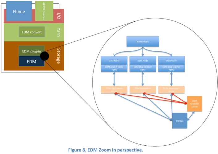
Considering the simulation process, it can be considered that all cluster nodes will run the entire number of time steps. The solvers will send their data to the platform by means of the Data Injector building block (a detailed explanation of this component is provided in section 5.1). They write results in GID‐format or HDF5. The result data for completed time steps will be extracted from the HPC while the remaining simulation time steps are still being processed. Figure 8 shows how the result data are then converted to AP209, merged and stored into EDM DB.

(17)

The conversion into AP209 is done before they are imported into EDM. The EDM DB may be located centrally or distributed over several cluster nodes, whatever gives best performance. The merge may be done either right behind the solvers (Map/reduce and HBase) or after the import into EDM; EDM has specific merge functionality. In the case of CIMNE solver, GID has already a method to merge data in GID‐format, but that works only on single cluster nodes. Data Injector includes a set of synchronizers that will store the raw data without merging into HBase. From there they may be read and converted for storage in AP209/EDM by means of EDM plugin.

Data shall be permanently stored in the most efficient way. EXPRESS and EDM seem to be an appropriate solution for standards compliant data. Files of proprietary formats can also be stored in EDM.

The existing visualization engines GiD and iFX will retrieve the result data by real‐time and batch queries from the distributed EDM by means of the EDM plugin building block which will provide a query solver based on Hadoop.

3.3.2 Viewbasedonafullopensourcesoftwarestack.

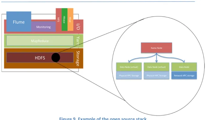
In this architectural view all the components are included in the open source platform. With this strategy, the full power of the Hadoop ecosystem is released: the system is based on file the storage system, and all the plugins have already been efficiently developed and disseminated worldwide for such all kind of data. Also, a huge client base exists today worldwide including IT giants, e.g., Google, Yahoo, Amazon, to name a few.

In this example Figure 9, the Flume agent performs the data gathering. Data is stored into HDFS using the Hbase data layout. Hive can be extended to store data into an Hbase format. And Flume agents can be connected to the HBase storage system. A multi‐resolution agent creates different levels of detail for each dataset. The physical storage used is based on HDFS. In this architecture, for the query model, two layers are available: one using Hive and the other using Hbase. Computation is performed using the new computation scheduler of Hadoop named YARN [5].

(18)

Figure 9. Example of the open source stack

For the visualization software, the connection to the platform is performed using an extension based on the Thrift tool [7]. Thrift is able to provide all the necessary classes to create a client server application, using any computer programming language.

Moreover, to increase the computation capabilities of such a solution, it is possible to use virtualization based on Linux “containers” [9], which, based on our experiments, brings a higher efficiency than virtual machines, e.g., Virtual Box [8]. Except for the Flume agent, this architecture is already deployable using our Hadoop deployment tool.

All these components have been validated during a comparative study, and usages of both plugins (Hive and Hbase) are relevant. Hbase is more suitable to extract specific content from a dataset, while Hive is more relevant for extracting a whole dataset. In a current paper [6], we are making an evaluation of three of these components for read operations on different architectures: Hive, Hbase and NFS, using both containers and virtual machines for performance comparisons [6].

(19)

4. HPC

Simulation

Infrastructure

The first prototype of VELaSSCo platform will be installed and tested in two dedicated nodes that have already purchased. The specifications of theses nodes are described in Table 1. These two nodes are already installed and working in the framework of Eddie cluster of the Edinburgh Compute and Data Facility (ECDF), the institutional service provider of High Performance Computing and Research Data Services to the University of Edinburgh.

The Eddie cluster is composed of worker nodes that run an industry standard Linux based operating system, specifically Scientific Linux release 6.5. Currently, Eddie cluster comprises two main parts:

 Mark2Phase1 ‐ 130 IBM dx360M3 iDataPlex servers, each with two Intel Xeon E5620 quad‐core processors. All these nodes are connected by a GigabitEthernet network with a 10 Gigabit network core.

 Mark2Phase2 ‐ 156 IBM dx360M3 iDataPlex servers, each with two Intel Xeon E5645 six‐core processors. All these nodes are connected by Gigabit Ethernet network, and 68 of them are also connected by a QDR QLogic Infiniband network‐ for Message Passing Interface (MPI) jobs.

Eddie can also deal with distributed memory parallel tasks where fast inter‐node communication is required. The Infiniband equipped portion is especially suited to this role. There are 68 nodes in this section giving the capability to run up to 816 way parallel jobs, although in general we expect that most such jobs will utilize 256 or fewer cores.

Eddie is connected to a large amount of high performance disk storage via a number of dedicated machines. These machines then share the data across the cluster using a parallel file system. For VELaSSCo platform, it is planned up to 200TB (currently 50 TB) of data storage as working capacity for visualization of data sets, with data backup for appropriate project golden copy data and dedicated LTO6 tape jukebox to ingest the provided data sets. The use of a dedicated tape jukebox will allow easy ingest of data, while a high bandwidth connection with the ECDF “Eddie” cluster and the HECToR and ARCHER UK supercomputers will allow easy transfer of data to and from high‐performance HPC storage.

CPU 2 x Intel Xeon ES‐2680v2 2.8GHz (10‐core, 20‐threads) RAM 384 GB RDIMM, 1600 MHz RAM

Hard disks 2 x 146 GB, SAS 15K RPM Hard drive 2 x 1.2TB SAS 10K RPM Hard drive

External storage 50 TB (extendible up to 200 TB) of Network‐Attached Storage (NAS)

(20)

5. Big

Data

Framework:

Data

Injection,

Storage

and

Computation

As it was described in detail in section 3, the core of the VELaSSCo architecture is the Big Data Framework in which the VELaSSCo is based on. From the functional point of view the Big Data framework will provide support for data injection, storage for raw data and computation. Next subsections provide a detailed description of each one of these functional blocks.

5.1.Data Injection

Data injection functionality will be provided by Atos through DataBlaster REST service, which basically aims to receive the input data from different simulations, managing and splitting them into different threads to optimize the process and finally store this information into a database. Figure 10 displays the three main blocks which compose the workflow:

 Simulation Input data represents the information generated by each simulation process and sent to the event manager through the API REST service.

 The Event Manager is implemented with Flume which basically allows multiplexing the input into different pipelines.

 And finally the HBase table, which is created to store the information delivered by Flume after processing.

5.1.1 ApacheFlumePipelines

Apache Flume is a distributed and secure to collect, aggregate and move large volumes of data from different sources logs from a centralized data warehouse system.

Using Apache Flume not only adheres to the aggregation of data from logs. Because data sources are configurable, allowing Flume be used to collect data from events related to network traffic, social networking, e‐mail messages to almost any possible data source.

The use of Flume within VElaSSCo will focus on providing the required pipelines to process simulation data created, in order to split it efficiently in several pieces that will be eventually stored in a NoSQL database, in a predefined schema. To do so, one

Simulation

Input Data Event Manager

HBase

table

(21)

of the requirements on VELaSSCo is creating one or multiple agents with Flume to synchronize on HBase repository. To do so, the pipelines are provided after multiplexing channels for agent. This is the case when we want to use the same agent over different channels to communicate sources and sinks like in Figure 11:

Figure 11. Flume multiplexing channels.

To do so, we need to change configuration file for every different channel: # cat conf/channel1‐flume‐conf.properties:

agent.sources=avroSource agent.channels=memoryChannel agent.sinks=hbaseSink agent.sources.avroSource.type=avro agent.sources.avroSource.channels=memoryChannel agent.sources.avroSource.bind=0.0.0.0 agent.sources.avroSource.port=61616 agent.sources.avroSource.interceptors=i1 agent.sources.avroSource.interceptors.i1.type=timestamp agent.channels.memoryChannel.type=memory agent.sinks.hbaseSink.type=hbase agent.sinks.hbaseSink.channel=memoryChannel agent.sinks.hbaseSink.table=velassco_simuldata # filling first column

agent.sinks.hbaseSink.columnFamily=simulationInfo agent.sinks.hbaseSink.batchSize = 5000

(22)

Also we need to add specific sink in order to split the input into different table columns:

# splitting input parameters

agent.sinks.hbaseSink.serializer=org.apache.flume.sink.hbase.RegexHbaseEventSeri alizer

agent.sinks.hbaseSink.serializer.regex=(.+)-(.+)-(.+)$

agent.sinks.hbaseSink.serializer.colNames=simulId,resultPart,raw_data

Therefore, the Event Manager used is Flume, so the pipelines are created multiplexing different channels for the same agent, assigning different port for each one of the pipeline. Figure 12 represents the pipelines within the event manager:

5.2.Data Storage

The current section provides a detailed description about the different types of storage included in the VELaSSCo architecture based on NON SQL in the case of Simulation Raw Data and based on EXPRESS (ISO 10303) in the case of AP209.

5.2.1 HBaseasNONSQLStorageforrawdata

Apache HBase is the Hadoop database, a distributed, scalable, big data store. Apache HBase use is recommended when you need random, real‐time read/write access to your Big Data. The use of HBase on VELaSSCo is dedicated to store the output data return from Flume through the different pipelines. To store this information, first it is necessary create a schema like Hbase table with the required column fields:

 create ‘velassco_simuldata’,’simulation_info’

Concretely, the fields which are going to be stored here are:

o simulId: Identifer of simulation part

Flume Event Manager

port1 port2 portN Data Source1 Source2 SourceN Channel1 Channel2 ChannelN HBaseSink1 HBaseSink2 HBaseSinkN Figure 12. Flume Event Manager.

(23)

o partNumber: The number of the part stored

o Sim_raw_data: this is the raw data to be stored. It could be a large amount of information so it is important to divide it into several pieces.

All the fields described above are store into a single column called ‘simulation_Info’. VELaSSCo simuldata database has been created in order to store separately every set of data sent through flume into different columns. The main goal is being able to deal with concurrent access to database to store a large number of registries with fields described above in ‘simulation_info’ column:

For example, one registry would look like:

rowkey ‐ timestamp simulation_info 1410192283757‐ GkbXAwHY7V‐7 Show 1 Timestamp simulId: 001 partResult: Welcome

raw_data: Flume is a distributed, reliable, and available service for efficiently collecting, aggregating, and moving large amounts of log data.

In row registry above, it is displayed the rowkey – timestamp auto generated when data was inserted and ‘simulation_info’ columns with field values for simulId, partResult, raw_data. Example of different registries stored in velassco_simuldata:

(24)

5.2.2 EDMHadoopPlugin

The EDM Hadoop plugin can be implemented along the same pattern as the current implementation of the EDM web services. The main building blocks of this implementation are a web server front end and the EDMserver™. The front end to the server is implemented as servlets in a Tomcat web server. See the Figure 13:

Figure 13 ‐ Current EDM web service implementation

The servlets communicates with the EDMserver™ via two .dlls, one .dll that is the bridge between the Java code in the servlets and the general client module for communication with

the EDMserver™, EDMinterface™.

The Hadoop EDM plugin will use the general Java interface to the EDMserver™. This interface is named EDOM3 and makes all server functionality available to a Java client program. See Figure 14 . The Hadoop EDM plugin will then consist of the following modules:

1. Java module that implements the Hadoop / EDMserver™ interface using EDOM3. 2. The EDOM3 Java layer.

3. JNI (Java Native Interface) based module to communicate between the EDOM3 Java layer and EDMinterface™.

4. EDMinterface™. This is the general interface for clients that will communicate with

an EDMserver™. Machine / HPC node User program Tomcat Web Service front end EDM application server EDM application server EDM application server EDM application server EDM application server User programUser programUser programUser program EDMremoteExecute WebService SOAP

(25)

Figure 14 ‐ VELaSSCo platform with Hadoop and EDM plugin With the EDOM3 Java interface the Hadoop EDM plugin can:

 Create and delete databases

 Create and delete repositories and data models (data sets).  Execute queries on selected data models

 Upload and download STEP (P21 and P28) files to/from data models.  Retrieve database dictionary information.

 Install and compile Express‐X programs

The domain that is simulated is divided into several sub‐domains. The simulation of one sub‐ domain is executed on one HPC node. JOTNE proposes that the results of the simulation of one sub‐domain are stored in one EDM data model (dataset). Each data model will contain the results from all time steps. All the data models from one simulation are contained in one EDM repository. This repository must also contain one data model that contains "global data" like type of simulation, name, description, dates, owner etc. and a list of the sub‐ domain data models.

Injection of new "result time‐step slices" while displaying previous results can be implemented by having two EDM application servers pr. EDM data model (sub‐domain). One serves the display queries and one adds new "result time‐step slices".

The visualization query mechanism will be implemented as a C++ plugin to the EDM application server. The visualization engine executes database queries by executing methods in the server side C++ plugin. For example, a query that returns the necessary data for visualization of a cut plane may in C++ look like:

CutplaneData *VELaSSCoViewer::getCutPLaneData(...) { ... } Machine / HPC node

Hadoop

EDM app server Machine / HPC node EDMinterface™protocol Hadoop EDM Plugin -EDOM3

EDM bridge - JNI EDMinterface™

VELaSSCo visualization program VELaSSCo visualization program C++ plugin EDM app server C++ plugin EDM app server C++ plugin EDM app server C++ plugin EDM app server C++ plugin EDM app server C++ plugin

(26)

Inside this method there can be a call to the VELaSSCo server that in the EDM way can look like:

edmiRemoteExecuteCppMethod(

pluginName, // string ‐ .dll file name methodName, // string

targetDataset, // specification of the datasets to be accessed mapSpecifications, // data that is used to divide query into sub‐queries Input parameters // binary data (blob)

Memory allocator(s) – for return values Return values // binary data (blob) );

The input data edmiRemoteExecuteCppMethod is the input parameters to VELaSSCoViewer::getCutPLaneData(...) serialized to a binary data set (blob) ready for transfer to the server. Likewise is the return values from the query a blob that must be deserialized inside VELaSSCoViewer::getCutPLaneData(...). If the input parameters and the return values are bigger than a certain limit, the data will be compressed before sending and decompressed at the receiving site.

In the VELaSSCo platform the edmiRemoteExecuteCppMethod call shall be started in all EDM application servers that shall take part in the execution. The execution of the edmiRemoteExecuteCppMethod on the client will call Hadoop in some way. And Hadoop shall then distribute the input parameters to all EDM application servers.

Pre‐computed data sets can be stored in the EDM database as an EDM file attribute which is binary data stored in separated files in the database folder. By this mechanism it is very easy to access pre‐computed data sets.

How the data shall be returned to the Visualization engine is an open question. Shall the Visualization engine know that the simulation domain is divided into sub‐domains? And, if so, shall it receive the query result from each sub‐domain separately?

The EDM Hadoop Plugin shall also be possible to plug into Flume. There the data to be ingested to the VELaSSCo database will be sent to the EDM server as input parameters to an ingestion method in the server side C++ plugin.

5.2.3 Eventsgeneratedbythedataingestion

When a simulation program ingest data into the VELaSSCo platform several queries will be automatically triggered in order to already have pre‐computed information when the user interacts with the simulation models stored in the platform.

This is the list of the queries that will eventually be triggered by the Data Ingestion module, from the Data Layer, depending on the type of the ingested data:

(27)

 Model information summary: with name, number of partitions, Bounding Box of the domain, mesh and result information (number of nodes, elements, time‐steps and result names), and validation status initialized with default value.

 Discrete to continuum transformation, with default parameters.  One, or more, simplified versions of the simulation model

 Pre‐compute some frequent user queries detected by the data pattern detection/identification mechanism.

(28)

6. Query

Manager

The Query Manager (QM) module of the VELaSSCo.QueryEngine.Layer is responsible of:  receive and manage VELaSSCo queries

 ensure feed‐back to the user

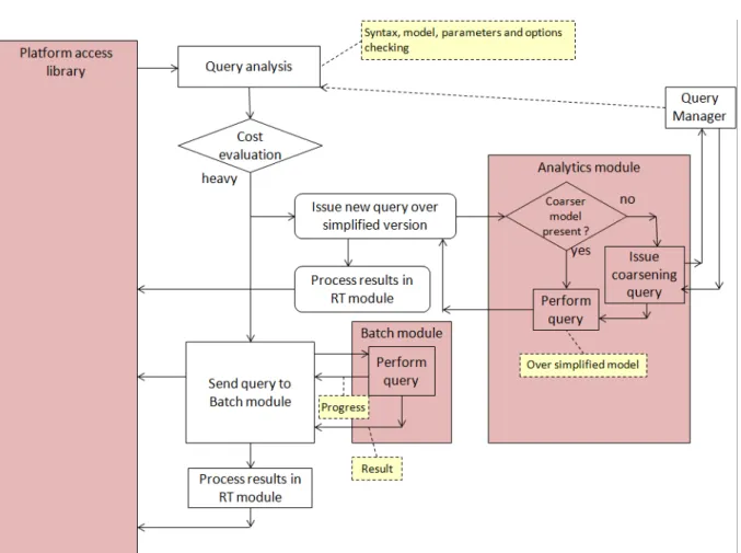
When receiving a VELaSSCo query from the visualization client the QM will evaluate the cost of executing this query. If the cost is small, them it will pass the query to the analytics module and receive the results of the query from the Real Time module and send the information back to the visualization client.

If the query is too heavy, then it will pass the query to the batch module and ask the analytics module for a simplified evaluation of the query, i.e. to evaluate the query over a simplified version of the simulated data. If the simplified version of the simulation model does not exist, then it will issue a coarsening query to generate a simplified version of the simulation model. The QM will receive result of the query over the simplified version and the progress of the batch queries and forward them to the user. At any moment the query may be stopped by the user, then the QM will stop the batch query evaluation but not the coarsening query if it has been generated, as the simplified version of the simulation model may be need for other queries. Figure 15 and Figure 16 display the workflow of both cases.

Figure 15. Steps to follow when processing light VELaSSCo queries

(29)

Figure 16. Steps to follow when processing heavy VELaSSCo queries

(30)

7. Data

Analytics

The data analytics module of the VELaSSCo.QueryEngine.Layer will perform the data analytics over the stored simulation results. It will also provide a cost estimation of the data analytic query to help the Query Manager evaluate in which mode is the analytics to be evaluated: in Speed mode or in Batch mode. This module also contains the coarsening algorithms to build simplified versions of the simulation data in order to provide fast feedback to the user and the Discrete to continuum transformation needed by the DEM simulation data. These two lasts processes will be launched by the Data ingestion module of the data layer or by the query manager module depending on user parameters or the need to provide feed‐back to the user.

The first VELaSSCo queries to be implemented will help determine the proper formats of communication between the different modules of the different layers and the libraries to access the platform. It will also help to further experiment with the platform and choose the proper tools, and their configuration for the correct and efficient execution of VELaSSCo queries and access and storage of the simulation data.

The list of the first queries is:  Session connection:

o Validation

o List of models for model selection: with some of the already gathered information: with name, number of partitions, Bounding Box of the domain, mesh and result information (number of nodes, elements, time‐steps and result names), validation status

 Model view:

o Get already existing groups/layers (Surfaces, line meshes of DEM particles) o Extract skin of Volume meshes, and store it,

o Store a thumbnail of the simulation model,

o Change the validation status of the model  Results view:

o Get list of analysis, steps and result properties (name, type, location, …) present in the simulation model,

o Given a list of nodes or elements, and a result identification (name, step, analysis) get the result values for those nodes or elements,

o Given a point in space and a result identification (name, step, analysis) interpolate and get the result value,

o Discrete to continuum transformation (DEM) according to default/provided parameters, as fast/light query and as batch/heavy query, to help evaluate cost of queries and implement batch module). Also store this transformation in the Data Layer.

(31)

These are common queries for both FEM and DEM type of simulation data.

For the 'Session connection' queries, a user identification will be needed to check permissions, and, eventually, maintain and store user‐related model‐independent data (like permissions, name …) or model related data, like thumbnails, used queries (like cut‐planes definitions, iso‐surfaces values, …)

To provide information in the model selection step, some information will be stored together with the simulation model. This information includes name, number of partitions (i.e. parts used in the distributed computing of the simulation problem), Bounding Box of the domain, mesh and result information (number of nodes, elements, time‐steps and result names), validation status. This information should be calculated and stored when the data is ingested in the platform for a faster interaction with the user in the model selection step. The 'Model view' and 'Result view' queries listed above for the 'first platform iteration' will define the specific data‐queries to the HadoppAbstractFileSystem (HAFS) and both storage solutions (HDFS and EDM). These data queries will be used widely in almost all following VELaSSCo queries and thus should be implemented in the most efficient way, but avoiding too much specialization.

The simulation user may define his own names and descriptions for analysis, mesh groups, results. May be these names are also translated into other languages. So instead of implementing the data query HAFS.getDisplacementsForNodes(…), the data query footprint should be:

HAFS.getResultForNodes(ModelHND: reference to the user selected model,

ResultName: String, ResultStep: String/Double, ResultAnalysis: String, listOfNodesId:

listOfIntegers) returns ResultValues: listOfDoubles

if result is a scalar, then ResultValues.size() == ListOfNodesId.size()

if result is a vector, then ResultValues.size() == ListOfNodesId.size()*3 (x, y, z)

ir result is a matrix, then ResultValues.size() == ListOfNodesId.size()*6 (Sxx, Syy,

Szz, Sxy, Sxz, Syz)

The same is valid for mesh/group names …

On a further iteration, the result of the 'skin extraction' query may be stored together with the model.

Thumbnail and validation status of the model may be stored together with the model and can be different depending on the user.

Following sections list the queries grouped functionalities for the first prototype and the final prototype, as described in the D1.3a deliverable.

The listed queries will provide a cost estimation method to help the QueryManager evaluate the cost of executing the query and perform the proper actions: execute it, or issue a simplified version of the query and send it to the batch module.

(32)

Depending on the experiments the details of the queries may vary to reduce latencies and bandwidth requirements and ensure the interactivity with the user.

7.1.FEM data analytics

Queries applied to FEM simulation data are: 1) Mesh queries:

 getMeshGroupList(ModelId): returns a list of the mesh groups present in the selected

simulation model with their properties: name, eventually colour, number and type of elements.

 getMeshData(ModelId, MeshName): returns a list of nodes and elements of the

mesh. This query may be spitted eventually into several sub‐queries like: getGlobalMeshCoordinates, getMeshCoordinates, getMeshElements, etc.

 getBoundaryMesh(ModelId, MeshName): returns the boundary (skin) of the volume

mesh: a list of triangles and/or a list of quadrilaterals, depending if the volume mesh has tetrahedra, hexahedra, prisms or pyramids. If it's not present calculates the boundary mesh it together with the simulation model and returns it. Depending on the calculation cost, this skin may be stored together with the simulation model.

 getNodeList(BoundingBox): returns a list of nodes (id and coordinates) inside the

bounding box.

 getElementList(BoundingBox): returns a list of elements (ids) inside the bounding

box.

 doCutPlane/Line/Segment(cutcoefficients): performs a cut on the simulation model

using the plane, line or segment coefficients and returns a list of triangles, lines with their coordinates.

 getBoundaryConditions(): returns a list of (String and element id's or node id's) of the

placed conditions on the simulation model

 deleteModel(ModelId): delete a simulation model (original, simplified or discrete‐to‐

continuum transformed)

 deleteMesh(MeshName): deletes a mesh of the simulation model

2) Result queries:

 getAnalysisAndStepList(model): returns, for the user selected model, the list of

analysis and for each analysis a list of the steps present in the analysis.

 getResultList(model, analysis, step): returns a list of result information for the results

present in the provided step. This information contains the result's name, result's type, components names and units, among others.

(33)

 getResultsForNodes(model, analysis, step, result name, component name/all, list of

nodes id's): returns a list of the results values for the provided nodes id's.

 getResultsForElements(model, analysis, step, result name, component name/all, list

of elements id's): returns a list of the results values for the provided nodes id's.

 getResultForPoint(model, analysis, step, result name, component name/all,

coordinates): returns the interpolation of the result for the provided coordinates.

Eventually a variant of this query may be implementer for a list of coordinates where the result is to be interpolated.

 doCutPlane/Line/SegmentWithResult(cutcoefficients, analysis, step, result name,

component name/all): performs a cut on the simulation model using the plane, line

or segment coefficients and returns a list of triangles, lines with their coordinates, and result values on the coordinates.

When the user performs a cut plane and changes the result visualized, several doCutPlane/doCutPlaneWithResult queries may be launched with the same cut coefficients. This may be inefficient. Depending on the experiments or a more close analysis, a variant, or variants of these queries will be implemented:

one with temporary objects:

CutObjectId coi = doCutPlane(parameters)

results = interpolateResults(coi, result name 1, …) results = interpolateResults(coi, result name 2, …) results = interpolateResults(coi, result name 3, …) deleteCutObject(coi);

or returning more information, including nodes and elements of the original mesh which are crossed my the cut‐plane, with their interpolation factors) to visualization client:

InterpolationInformation localCutInfo= doCutPlane(parameters)

tmp = getResultsForNodes(localCutInfo.originalNodes, result name 1, …)

results = local_interpolate(localCutInfo, tmp);

results = local_interpolate(InterpolationInformation, tmp);

results = local_interpolate(localCutInfo, tmp); or returning more information to visualization client

Visual Analysis for Extremely Large Scale Scientific Computing

Visual

Analysis

for

Extremely

Large

‐

Scale

Scientific

Computing

D2.2

–

Specification

of

Big

Data

Architecture

Table

of

Contents

1.

Introduction

2.

Concepts

of

VELaSSCo

Architecture

3.

Specification

of

VELaSSCo

Architecture

4.

HPC

Simulation

Infrastructure

5.

Big

Data

Framework:

Data

Injection,

Storage

and

Computation

Hadoop

6.

Query

Manager

7.

Data

Analytics