Single-symbol and Double-symbol Decodable STBCs for MIMO Fading Channels

(1)

Single-symbol and Double-symbol Decodable STBCs

for MIMO Fading Channels

A Thesis

Submitted For the Degree of

Doctor of Philosophy

in the Faculty of Engineering

by

Md. Zafar Ali Khan

Department of Electrical Communication Engineering Indian Institute of Science

Bangalore – 560 012 JANUARY 2005

(2)

For a communication system operating in a fading environment, receive antenna diversity is a widely applied technique to reduce the detrimental effects of multi path fading. But as this makes the receiver complex and costly, is generally used exclusively at the base station. Recently a combination of transmit and receive diversity has been suggested as a more effective solution to the above problem resulting in a MIMO (Multiple Input Multiple Output) fading channel which has been shown to have the potential of supporting large data rates as compared to SISO (Single Input Single Output) channels. Signal design for such a MIMO channel is known as Space-Time Codes (STC), which take advantage of both space and time diversity available with time varying fading by coding both in space and time.

Space-Time Block Codes (STBC) are promising in this regard as there exist fast decoding algorithms like sphere decoding, etc. Further there exist classes of codes among STBCs that have very simple decoding properties like STBCs from orthogonal designs (ODs) and quasi-orthogonal designs (QODs). This simplicity of decoding for ODs and QODs is due to the fact that the Maximum Likelihood (ML) decoding metric can be written as sum of squares of terms each depending on only one variable in the case of OD and two variables in the case of QODs; as a result each variable can be decoded separately for ODs and pairs of variables for QODs. However the rates of ODs and QODs are restrictive; resulting in search of other codes. It is in this context that STBCs are investigated in this thesis where we classify and characterize all STBCs that have decoding properties similar to ODs and QODs; calling them “single-symbol decodable (SD)” and “double-symbol decodable (DSD)” respectively, for quasi-static and fast-fading channels when channel state information (CSI) is known at the receiver.

The characterization of symbol decodable STBCs shows that full-rank single-symbol decodable designs can exist outside the well-known Generalized Linear Processing

(3)

Complex Orthogonal Designs. In particular, we present single-symbol decodable, full-rank, rate 1, space-time block codes (STBCs) for 2 and 4 antennas that are not-obtainable from GLCODs.

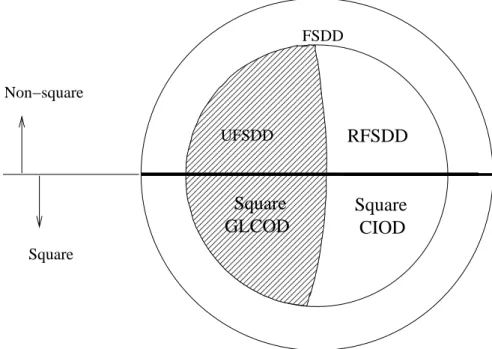
The characterization of single-symbol decodable STBCs proceeds in two steps: first, we characterize all linear STBCs, that allow single-symbol ML decoding (not necessarily full-diversity) over quasi-static fading channels-calling them single-symbol decodable designs (SDD). The class SDD includes GLCOD as a proper subclass. Among the SDD those that offer full-diversity, called Full-rank SDD (FSDD), are characterized. For square FSDD, complete classification and construction of maximal rate designs are presented. As a consequence, we show that full-rank, rate-one, square SDD exist only for 2 and 4 transmit antennas and GLCODs are not maximal rate FSDD except for N = 2.

For non-square FSDD we present a class of non-GLCOD, STBCs called Generalized Co-ordinate Interleaved Orthogonal Designs (GCIODs). Construction of various high rate (>1/2) designs within this class of codes is presented and the coding gain and maximum mutual information (MMI) of these codes is evaluated and compared with known STBCs. We then show that the class of GLCODs and GCIODs arise naturally when all maximal SNR STBCs are characterized.

A characterization of all double-symbol decodable STBCs is then presented, in par-ticular we present a double-symbol decodable, full-rank, rate 1, STBCs for 8 antennas. Next, we propose designs for fast-fading channels and derive maximal rates of single, double symbol decodable designs for fast-fading channels. Of particular interest is the uniqueness of CIOD for 2 Tx. which has single-symbol decodability for both quasi-static and fast-fading channels.

It turns out that co-ordinate interleaving of complex constellations is an effective tool to improve the diversity performance of MIMO fading channels without accruing any complexity penalty at the receiver.

(4)

I am grateful to my parents and family for their patience andlove; but for their counsel and support (moral, financial) in very difficult circumstances, I could not have even thought of joining Ph.D.

I would like to thank Prof. B. Sundar Rajan, my supervisor, for his many suggestions and constant support during this research.

Thanks are due to Shashidhar, Bikash, Viswanath, Nandakishore and Kiran for their counsel (both technical and non-technical) and company. Thanks are also due to my lab-mates ( Sripati, Manoj, Subbu, Chandru etc.) who made my stay enjoyable. Thanks are again due to all those who helped me throughout my stay at IISc.

I would also like to thank Teku and MT of SASKEN for their encouragement and help in joining the Ph. D. program at IISc.

(5)

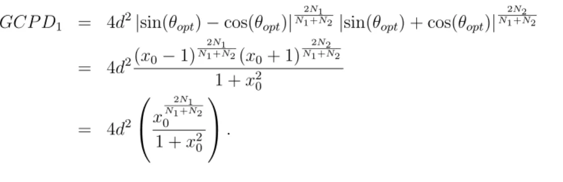
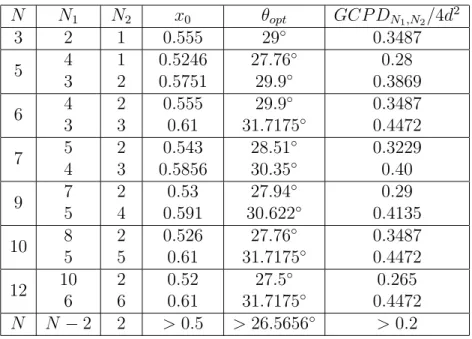
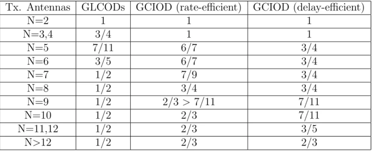
3.1 The Encoding And Transmission Sequence For N =2, Rate 1/2 CIOD . . . 50 3.2 The Encoding And Transmission Sequence For N =2, Rate 1 CIOD . . . . 51 3.3 Comparison of rates of known GLCODs and GCIODs for allN . . . 62 3.4 Comparison of delays of known GLCODs and GCIODs N _≤8 . . . 62 3.5 The optimal angle of rotation for QPSK and normalized GCP DN1,N2 for

various values of N =N1+N2. . . 76

3.6 The coding gains of CIOD, STBC-CR, rate 3/4 COD and rate 1/2 COD for 4 tx. antennas and QAM constellations . . . 81 A.1 Comparison of coding gains of ACIOD and OD for N = 3 . . . 169

(9)

List of Figures

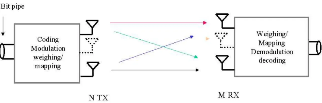
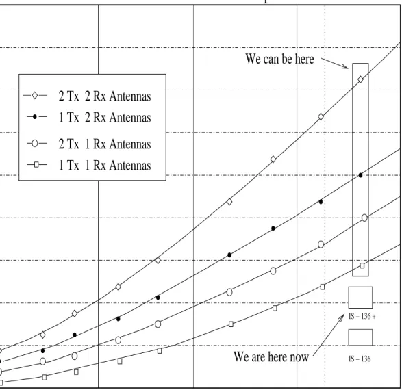
1.1 Diagram of a MIMO wireless transmission system. . . 2 1.2 The outage Capacity, C0.99, for various combinations ofN = 2,1 andM =

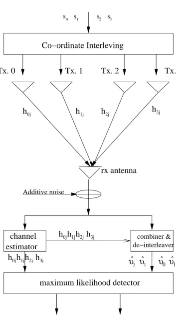
2,1 MIMO systems in Rayleigh fading . . . 5 2.1 The classes of single-symbol decodable (SDD) codes. . . 19 3.1 Baseband representation of the CIOD for four transmit and thej-th receive

antennas. . . 52 3.2 Expanded signal sets ˜_A for _A=_{1,₋1,j,₋j_} and a rotated version of it. . 64 3.3 The plots ofCP D1, CP D2 for θ∈[0 90◦]. . . 72

3.4 The BER performance of coherent QPSK rotated by an angle of 13.2825◦

(Fig.3.2) used by the CIOD scheme for 4 transmit and 1 receive antenna compared with STBC-CR, rate 1/2 COD and rate 3/4 COD at a through-out of 2 bits/sec/Hz in Rayleigh fading for the same number of transmit and receive antennas. . . 82 3.5 The BER performance of the CI-STBC with 4- and 16-QAM modulations

and comparison with ST-CR and DAST schemes . . . 83 3.6 The maximum mutual information of CIOD code for two transmitters and

one, two receiver compared with that of complex orthogonal design (Alam-outi scheme) and the actual channel capacity. . . 87 3.7 The maximum mutual information of GCIOD code for three transmitters

and one, two receiver compared with that of code rate 3/4 complex orthog-onal design for three transmitters and the actual channel capacity. . . 88 3.8 The maximum mutual information of CIOD code for four transmitters and

one, two receiver compared with that of code rate 3/4 complex orthogonal design for four transmitters and the actual channel capacity. . . 89 3.9 The maximum mutual information (average) of rate 2/3 GCIOD code for

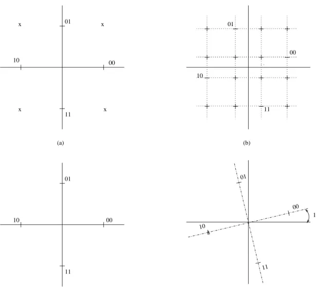
eight transmitters and one, two, four and eight receivers compared with that of code rate 1/2 complex orthogonal design for eight transmitters over Rayleigh fading channels. . . 92 4.1 The signal constellations considered in Chapter 4. Except (c) all others are

(10)

5.1 The classes of double-symbol decodable (DSDD) codes. . . 119 5.2 The BER performance of coherent QPSK rotated by an angle of 13.2825◦

(Fig. 3.2 )for of the CIOD scheme for 4 transmit and 1 receive antenna compared with QOD in Rayleigh fading for the same number of transmit and receive antennas. . . 136 5.3 Expanded signal sets ˜_A for _A=_{1,₋1,j,₋j_} and a rotated version of it. . 142 5.4 The BER performance of STBCs from OD, QODs and the Quasi-CIOD for

N = 8 at 1.5 bits/sec/Hz in quasi-static Rayleigh fading channel. . . 143 6.1 BER curves for Alamouti and CIOD schemes for a) QPSK and b) BPSK

over varying fading channels where the probability that the channel is quasi-static is pand single-symbol decoding. . . 155

(11)

Abbreviations and Notations

MIMO multiple-input, multiple-output MISO multiple-input, single-output SIMO single-input, multiple-output SISO single-input, single-output TX,Tx transmit antennas

RX,Rx receive antennas

BER bit error rate

SER symbol error rate

ML maximum likelihood

SNR signal to noise ratio PAR peak to average ratio CSI channel state information

MMI maximum mutual information

STC space-time codes

STTC space-time trellis codes STBC space-time block codes

QAM quadrature amplitude modulation

PSK phase shift keying

OD orthogonal design

QOD quasi-orthogonal design

GQOD generalized QOD

LCOD linear complex orthogonal design

(12)

LROD linear real orthogonal design

GLROD generalized linear real orthogonal design

RFSDD restricted full-rank single-symbol decodable design QCRD quasi-complex restricted design

UFSDD unrestricted full-rank single-symbol decodable design CIOD co-ordinate interleaved orthogonal design

GCIOD generalized co-ordinate interleaved orthogonal design ACIOD Asymmetric co-ordinate interleaved orthogonal design CPD co-ordinate product distance

GCPD generalized CPD

SD single-symbol decodable

SDD single-symbol decodable design

DSD double-symbol decodable

DSDD double-symbol decodable design

FSD full-rank SD

FSDD full-rank SDD

FDSDD full-rank DSDD

NLC Non-reducible lattice constellation

MZD minimum zeta-distance

GMZD generalized MZD

ECoM extended codeword matrix

EChM extended channel matrix

iid independent, identically distributed NLC non-reducible lattice constellation

(13)

Notations

, variable definition

C _{the field of complex numbers}

R _{the field of real numbers}

j √₋1

CL×N _{the set of all} _L_×_N _{complex matrices} xI,Re(x) real part of a complex number x xQ,Im(x) imaginary part of a complex number x

x∗ _{conjugate of a complex number} _x

|x_| absolute value of a real number x

CP D(x, y) the CPD between two complex numbers xand y =_|xI ₋yI_||xQ₋yQ_|

AT transpose of a matrix A

AH _{hermitian of a matrix} _A

det(A),_|A_| determinant of a matrix A tr (A) trace of a matrix A

|A_|+ product of non-zero eigen values of a matrix A

||A_|| Frobonius norm of a matrix A A−1 Inverse of a matrix A

IN N _×N identity matrix

B(S, S0₎ _{difference of the matrices} _{S, S}0_{, i.e.,} _S₋_S0

Γ(x) Gamma function

|S_| cardinality of a set S

(M)N M modN

P(E) probability of an event E

H(N)₋1 number of matrices in a Hurwitz family of order N E [X] expected value of a random variable X

(14)

Introduction

Wireless mobile communications is characterized by a very lossy and dispersive transmis-sion medium, the fading channel, that suffers from extreme random fades. In designing communication systems for the fading channel, the emphasis is on minimizing the effect of channel fluctuations. Diversity as a technique for minimizing the detrimental effects of channel fluctuations, has been known to the wireless community since decades. A funda-mental requirement of the diversity method is that a number of independent transmission paths be available to carry the message. Independent paths can be obtained by coding in time-like repeatedly sending the same signal; resulting in time diversity. Time-diversity results in transmission delay and bandwidth loss. Significantly, time-diversity depends on the mobility of the antennas to provide independent paths and as such is useless when both the receiver and transmitter are stationary [1, chap. 5]. Alternately coding/repetition can be in frequency, wherein the same message is transmitted over different frequencies. This results infrequency diversity. But again, frequency diversity results in loss of bandwidth. Polarization and angle diversity have also been proposed but in both the cases the number of diversity paths are limited to two and three respectively.

Antenna or space diversity was and is favored for mobile radio for a variety of reasons; in particular, it does not require additional bandwidth. Figure 1.1 presents a graphical presentation of space diversity, with both the transmitter and receiver being equipped with multiple antennas.

Till a decade ago, antenna diversity was synonymous with receive diversity, wherein multiple antennas were used for reception. The problem with receive diversity for mobile communications is that the receive antennas had to be sufficiently apart so that the signals received at each antenna undergoes independent fade. While this is easily implemented

(15)

2

Figure 1.1: Diagram of a MIMO wireless transmission system.

at the base-station, since the mobile unit needs to be small in size it becomes costly to implement this in the mobile unit[2]. In order to reap the benefits of antenna diversity in the down-link (base-station to mobile) transmit diversity and/or a combination of trans-mit and receive diversity, termed otherwise as a multiple-input multiple-output (MIMO) link, was recently considered, wherein both the receiver and transmitter are equipped with multiple antennas (TX and RX respectively). A key concept in space diversity is the

diversity order which is defined as the number of decorrelated spatial branches available at the receiver.

In a very short period of about five years MIMO has emerged as one of the most significant technical breakthroughs of modern communication and is poised to penetrate commercial wireless products and networks. In fact the Alamouti scheme is currently a part of W-CDMA and CDMA-2000 standards [2]. The reasons due to which MIMO has and is generating so much interest is many-fold. A properly designed MIMO system not only leads to improved quality of service (Bit Error Rate or BER) but also improved data rate (bits/sec) and therefore revenues of the operator (as is clear from the absolute gains in terms of capacity, reviewed in Section 1.1) . This prospect of performance improvement at no cost of extra spectrum is largely responsible for success of MIMO as a new topic of research. This thesis deals with one of the many open-problems in the area of signal design for MIMO channels; that of achieving simple decodability while retaining the diversity benefits, that have come to fore in these five years of active research.

(16)

1.1

The MIMO System

Consider the MIMO system shown in Fig.1.1. A compressed digital source in the form of a binary data stream is fed to a transmitting block encompassing error control coding and mapping to a complex signal constellation (M-QAM, M-PSK). The coding produces sev-eral separate symbol streams (not necessarily independent) each of which is mapped onto one of the multiple TX antennas. Mapping may involve linear spatial weighing of anten-nas (as in the case of channel feedback) or space-time coding [3]. After upward frequency conversion, filtering and amplifying the signals are launched into the wireless domain. At the receiver the signals are captured by possibly multiple antennas and demodulation and demapping operations are performed to recover the message. The selection of coding and antenna mapping can vary a great deal depending upon the application and is primarily decided by factors such as receiver and transmitter complexity, prior channel knowledge among other factors. Here we are interested in exploring the absolute gains offered by a single-user MIMO system and its special cases the SISO, SIMO and MISO systems, in terms of Capacity when perfect CSI (Channel State Information) is available at the receiver.

Consider the traditional SISO system. In a flat-fading channel, the capacity is achieved with continuous Gaussian input and it is [2, 3],

C=E[log₂ 1 +ρ_|h_|2] bits/sec/Hz (1.1)

where the expectation is over the channel realizations h and ρ = _σP2 is the average SNR

expressed in terms of the total transmit power P and the average noise power σ2_.

For a matrix channel ofN transmit andM receive antennas with continuous Gaussian input and Rayleigh fading the instantaneous capacity version of 1.1 generalizes to [3, 5, 6]

C(H) = log₂hdet1 + ρ NHH

Hi _bits/sec/Hz _(1.2)

where nowρ is the SNR for one receive antenna and His the N_×M channel matrix. In a SIMO system with M receive antennas the capacity is given by [3]

C(H) = log₂ 1 +ρ M−1 X i=0 |hi_|2 ! bits/sec/Hz (1.3)

(17)

1.2 Space-time Codes 4

wherehi is the channel gain fori-th RX and for a MISO system withN Tx, we have [5, 6]

C(H) = log₂ 1 + ρ N N−1 X i=0 |hi_|2 ! bits/sec/Hz. (1.4)

The ergodic mean capacity is obtained by taking expectation on the expression 1.2 with respect to H. Observe that the factor _Nρ ensures a fixed total transmit power. The important point to observe [5, 6] is that in (1.2) C increases linearly with min(N, M). while there is a logarithmic increase inC with respect toM in (1.3) and with N in (1.4). The increase in capacity w.r.t. SISO is evident in all the three cases. Interestingly C(H) is a random variable and averaging this over H leads us to the ergodic mean capacity. From the practical point of view, for a quasi-static channel, what is more useful is the outage capacity, Cp i.e. the capacity that is supported with a probability p defined by Outage capacity Cp: Channel capacity is higher than Cp for p% of the time.

P r_{C(H)>Cp_}=

Z _∞

H:C(H)=Cp

C(H)fH(H)dH=p

.

Fig. 1.2 gives the outages for various MIMO systems. Observe that the data rate is more than double for a 2_×2 MIMO system at all SNRs as compared to a SISO system.

1.2

Space-time Codes

The following subsection describes the channel model, coding, decoding and the per-formance criteria for MIMO systems employing Space-Time Codes (STC). The primary difference between coded modulation (used for SISO, SIMO) and space-time codes is that in coded modulation the coding is in time only while in space-time codes the coding is in both space and time and hence the name. Space-time Codes (STC) can be thought of as a signal design problem at the transmitter to realize the capacity benefits summarized in the previous section, though, several developments towards STC were presented in [7, 8, 9, 10, 11] which combine transmit and receive, much prior to the results on capacity. Formally, a thorough treatment of STCs were first presented in [12] in the form of trellis codes (space-time trellis codes (STTC)) along with appropriate design and performance criteria, a brief review of which is given in subsection 1.2.1 and 1.2.2 gives a review of STBCs from orthogonal designs.

(18)

IS − 136 + IS − 136

0

225

200

175

150

125

100

75

50

25

0

5

10

15

20

2 Tx 1 Rx Antennas

1 Tx 1 Rx Antennas

1 Tx 2 Rx Antennas

2 Tx 2 Rx Antennas

Achievable Data Rates with Multiple Antennas

Achievable Date Rate (kbits/sec) per 30 kHz Channal

SNR per Rx Antenna (dB)

We can be here

We are here now

Figure 1.2: The outage Capacity,C0.99, for various combinations ofN = 2,1 andM = 2,1

(19)

1.2.1

The Channel Model and Performance Criteria for STC

Let the number of transmit antennas be N and the number of receive antennas be M. At each time slot t, the complex signals, sit, i = 0,1,· · ·, N −1 are transmitted from theN antennas simultaneously. Lethij =αijejθij denote the path gain from the transmit antenna i to the receive antenna j, where j = √₋1. Assuming that the path gains are constant over a frame length L _≥ N, t = 0,_{· · ·}, L₋ 1, the received signal vjt at the antennaj at time t, is given by

vjt = N−1

X

i=0

sithij+njt, j= 0,_{· · ·}, M ₋1; t= 0,_{· · ·} , L₋1, (1.5)

which in matrix notation is,

V=SH+N (1.6)

where, withC _{denoting the complex field,}

V_∈CL×M _{is the received signal matrix,}

S_∈CL×N _{is the transmission matrix (also referred as codeword matrix),}

N_∈CL×M _{is the additive noise matrix, and}

H_∈CN×M _{is the channel matrix.}

The entries of N and H are complex Gaussian distributed with zero mean and unit variance and also are temporally and spatially white. Note that in V,S and N time runs vertically and space runs horizontally and hij is the entry in the ith row and the jth column of H. Recall that for a matrix A, AH _{represents the Hermitian (conjugate}

transpose) ofA,AT _{represents the transpose of}_A _and _|_A_| _{denotes the determinant of}_A.

If the transmission power constraint is given byE[tr_{SSH_}] =LN then

V =

r

ρ

NSH+N (1.7)

where ρ is the SNR at each receiver. Assuming that perfect channel state information (CSI) is available at the receiver, the decision rule for ML decoding is to minimize the metric L−1 X t=0 M−1 X j=0 vjt₋ N−1 X i=0 hijsit 2 (1.8)

(20)

over all codeword matrices S. In vector form we have

M(S),min

S tr (V−SH)

H₍_V₋_SH₎₌_k_V₋_SH_k2_. _(1.9)

This ML metric (1.8)/(1.9) results in exponential decoding complexity, because of the joint decision on all the complex symbolssitin the matrix S. LetCS denote the set of all

possible codeword matrices. Then the throughput rateRof such a scheme in bits/sec/Hz is _L1 log2(|CS|) and 2RL metric calculations are required; one for each possible transmission

matrixS. Even for modest antenna configurations and rates this could be very large. For a STTC zero padding at the end of each frame is done and Vector Viterbi algorithm [12] is used to perform the minimization.

Towards describing the diversity and coding gains, letP(S_→Sˆ) be the pairwise error probability of S being transmitted and wrongly decoded as ˆS for the receiver based on (1.8). The Chernoff bound on this error probability takes the form [12, eq. (9)]

P(S_→Sˆ)_≤ _n 1

|I+₄ρ_N(S₋Sˆ)(S₋Sˆ)H_|oM

(1.10)

whereI is the identity matrix. For large SNR’s (large values of ρ), (1.10) can be written as

P(S_→Sˆ)_≤ 1 Λ(S,Sˆ)₄ρ_N

!rM

(1.11) wherer is the rank of the difference matrix,B(S,Sˆ) =S₋Sˆ, and

Λ(S,Sˆ) =_|(S₋Sˆ)(S₋Sˆ)H_|1₊/r (1.12)

where _|A_|+ represents the product of the non-zero eigen values of the matrix A. The

minimum of the ranks of all possible pairs of codeword matrices is referred to as the

diversity gain and the minimum value of Λ(S,Sˆ) over all possible pairs of codeword matrices is referred to as thecoding gain. The above pair-wise probability of error analysis for a quasi-static channel leads to

Design Criteria for STC over quasi-static fading channels[12]

• Rank Criterion: In order to achieve full-diversity of N M, the matrix B(S,Sˆ) has to be full-rank for any two codewords S, Sˆ. If B(S,Sˆ) has rank r, then a diversity

(21)

gain ofrM is achieved.

• Determinant Criterion: After maximizing the diversity gain the next criteria is maximizing the minimum of Λ(S,Sˆ) over all pairs of distinct codewords.

1.2.2

Space-time block codes (STBC)

Definition 1.2.1 (STBC). AnN_×L(generally,L_≥N) space time block code (STBC)

C consists of a finite number _|C|ofN_×Lmatrices with entries from the complex field. If the entries of the codeword matrices take values from a complex signal setS or complex linear combinations of elements of S then the code is said to be over S. For quasi-static, flat fading channels a primary performance index of_C is the minimum of the rank of the difference of any two codeword matrices, called the rank of the code. _C is of full-rank if its rank is minimum ofL and N and is of minimal-delay if L =N. The rate of the code in symbols per channel use is given by 1_l log_|S|(|C|).

The study of space-time block codes (STBC) started with the paper by Alamouti [16] and their subsequent generalization in [13] and development in [17, 18, 19, 15, 20, 21, 22, 23] using the theory of Orthogonal Designs (OD) [24, 25, 26, 27]. Many other STBCs like STBCs from Quasi-Orthogonal Designs (QOD) [28, 29, 30, 31, 32, 33, 34], STBCs using unitary precoders [35, 36, 37, 38] and other STBCs like [39, 40, 41] etc. were developed.

We first review the definition and important results of ODs and QODs before contin-uing our discussion.

Definition 1.2.2 (Generalized Linear Complex Orthogonal Design (GLCOD)[13]).

A GLCOD1_in_k_{complex indeterminates}_x

1, x2,· · · , xkof sizeN and rateR =k/p,p≥N

is a p_×N matrix Θ, such that

• the entries of Θ are complex linear combinations of 0,_±xi, i = 1,· · · , k and their conjugates.

• ΘH_{Θ =}_D_{, where} _D _{is a diagonal matrix whose entries are a linear combination of}

|xi_|2_{, i}_{= 1,}_{· · ·} _{, k} _{with all strictly positive real coefficients.}

1

In [13] it is called a Generalized Linear Processing Complex Orthogonal Design where the word “Processing” has nothing to be with the linear processing operations in the receiver and means basically that the entries are linear combinations of the variables of the design. Since we feel that it is better to drop this word to avoid possible confusion we call it GLCOD.

(22)

Ifk=n=p then Θ is called a Linear Complex Orthogonal Design (LCOD). Furthermore, when the entries are only from _{±x1,±x2,· · ·,±xk}, their conjugates and multiples of j

then Θ is called a Complex Orthogonal Design (COD). STBCs from ODs are obtained by replacing xi by si and allowingsi to take all values from a signal set _A. A GLCOD is said to be of minimal-delay ifN =p.

Actually, according to [13] it is required that D = Pk_i₌₁_|xi_|2_I_{, which is a}

special case of the requirement that D is a diagonal matrix with the conditions in the above definition. In other words, we have presented a generalized version of the definition of GLCOD of [13]. Also we say that a GLCOD satisfies

Equal-Weightscondition if D =Pk_i₌₁_|xi_|2_I.

The Alamouti scheme [16], which is of minimal-delay, full-rank and full-rate is basically the STBC arising from the size 2 COD.

The main results regarding GLCODs are summarized below:

• when _A is a real constellation, then rate 1 square, real, Orthogonal Designs exist ONLY for N=2,4 and 8 [13].

• when _A is a complex constellation, Square/Non-square GLCODs exist ONLY for N=2 [13, 20, 22].

• when _A is a complex constellation, the maximal rates of Square GLCODs of size N = 2a_{b, b} _{odd, satisfying Equal-Weights condition is [15]}

R= a+ 1 N .

Observe that the maximal rate, when the GLCODs do not satisfy the Equal-Weights condition, is not known [22],

• the STBCs from GLCODs satisfying Equal-Weights condition are optimal SNR codes [17, 18, 19, 23].

In the case of QODs, several constructions are given in [28, 29, 31, 32, 30, 33, 34] but the fundamental questions of rate and existence of QODs has not been dealt with, to the best of our knowledge.

(23)

define now: Following the spirit of [15], by a linear STBC2 _{we mean those covered by the}

following definition:

Definition 1.2.3 ( Linear STBC). A linear design, S, is a L_×N matrix whose en-tries are complex linear combinations of K complex indeterminates xk = xkI +jxkQ, k = 0,_{· · ·}, K ₋1 and their complex conjugates. The STBC obtained by letting each indeterminate to take all possible values from a complex constellation_A is called a linear STBC over _A. Notice that S is basically a “design”and by the STBC (S,_A) we mean the STBC obtained using the design S with the indeterminates taking values from the signal constellation _A. The rate of the code/design3 _{is given by} _K/L _{symbols/channel}

use. Every linear design S can be expressed as

S= K−1

X

k=0

xkIA2k+xkQA2k+1 (1.13)

where_{Ak_}2_kK₌₀−1 is a set of complex matrices called weight matrices of S.

Throughout the thesis, we consider linear STBCs only and also we use the word “linear design” and “linear STBC” interchangeably with the understanding that the signal set,

A, in (S,_A) is understood from context or will be specified when necessary. Linear STBCs can be decoded using simple linear processing at the receiver with algorithms like sphere-decoding [42, 43] which have polynomial complexity in,N, the number of transmit antennas. But STBCs from ODs and QODs stand out because of very simple (linear complexity inN) decoding. This is because the ML metric of (1.9) can be written as a sum of several square terms, each depending on at-most one variable for OD and at-most two variables for QOD. However, the rates of both ODs and QODs are restrictive; resulting in search of other codes that allow simple decoding similar to ODs and QODs. We call such codes “single-symbol decodable” and ”double-symbol decodable” respectively. Formally

Definition 1.2.4 (Single-symbol Decodable (SD) and Double-symbol Decod-able (DSD) STBC). A single-symbol decodable STBC of rate K/L in K complex indeterminates xk = xkI +jxkQ, k = 0,_{· · ·} , K ₋1 is a linear STBC such that the ML decoding metric given by (1.9) can be written as a square of several terms each depending

2

Also referred to as a Linear Dispersion (LD) code [39]

3

Note that if the signal set is of size 2b _{the throughput rate}_R_{in bits per second per Hertz is related}

(24)

on at most one indeterminate. If (1.9) can be written as a square of several terms each depending on at most two indeterminates, then the STBC is said to be double-symbol decodable.

Examples of single-symbol decodable STBCs are STBCs from Orthogonal Designs (ODs) and examples of double-symbol decodable STBCs are the QODs. To elucidate further, consider the Alamouti code

S(x0, x1) = " x0 x1 −x∗ 1 −x∗0 #

where x0, x1 are signal points from some complex constellation A. That the Alamouti

code is a SD STBC can be verified as follows,

M(S(x₀, x₁)) = min x0,x1∈A tr (V₋SH)H(V₋SH)=_kV₋SH_k2 (1.14) = min x1,x2∈A kV₋S(x0,0)Hk2+kV−S(0, x1)Hk2 −tr VVH (1.15) = min x0∈A kV₋S(x₀,0)H_k2 + min x1∈A kV₋S(0, x₁)H_k2 (1.16)

and hence each variablex0, x1 can be detected separately (see Proposition 2.3.1 for more

details).

1.3

Motivation, Overview and Scope of the Thesis

Despite enormous interest and research in STBCs from ODs and QODs, to the best of our knowledge the following fundamental questions related to STBCs from designs either remain unaddressed or are not answered fully:

1. Are STBCs from ODs the only single-symbol decodable linear STBCs? 2. Are single-symbol decodable codes necessarily full-rank also?

3. What are the maximal rates of single-symbol decodable linear STBCs, with or without full-rankness?

4. If they exist outside the domain of ODs, are all of them optimal SNR codes? 5. Are STBCs from QODs the only double-symbol decodable linear STBCs? What

(25)

1.3 Motivation, Overview and Scope of the Thesis 12

6. Are STBCs with single/double-symbol decodablity for quasi-static channel useful, or in some sense related to STBCs suitable, for fast-fading channels?

The above questions are also precisely the set of issues addressed and answered/settled almost completely in this thesis. This is achieved by way of characterizing the entire class of SD and DSD STBCs, without out taking into account their full-rankness and then bringing the full-rankness into consideration. This thesis also deals with the various aspects of these designs including the diversity and coding gain with various signal sets.

The contributions of this thesis are presented in the form of following five chapters 1. Chapter 2: Single-symbol Decodable, Full-diversity Linear STBCs4

2. Chapter 3: Generalized Co-ordinate Interleaved Designs5

3. Chapter 4: Characterization of Optimal SNR STBCs

4. Chapter 5: Double-symbol Decodable Designs6

5. Chapter 6: STBCs from Designs for Fast-Fading Channels7

an outline of each of which follows:

Chapter2: Single-symbol Decodable, Full-diversity Linear STBCs

Space-Time block codes (STBC) from Orthogonal Designs (OD) has been attracting wider attention due to their amenability for fast (single-symbol decoding) ML decoding, and full-rate with full-rank over quasi-static fading channels [16]-[23]. Unfortunately, for complex constellations full-rate, full-rank, square ODs exist only for 2 transmit antennas and for larger number of antennas one needs to pay in terms of reduced symbol-rate or rank or not having single-symbol decodability.

It is natural to ask, if there exist codes other than STBCs form ODs that allow single-symbol decoding? In this chapter, this question is answered in the affirmative by showing that full-rank, full-rate and single-symbol decodable designs can exist outside the well-known Generalized Linear Complex OD (GLCODs) [13]. We first characterize all linear STBCs, that allow single-symbol ML decoding (not necessarily full-diversity)

4

Part of the results of this chapter are reported in the the publications [50, 52, 53, 55]

5

Part of the results of this chapter are reported in the the publications [50, 51, 52]

6

Part of the results of this chapter are reported in the the publications [53, 57]

7

(26)

over quasi-static fading channels-calling them single-symbol decodable designs (SDD). The class SDD includes GLCOD as a proper subclass. Among the SDD, those that offer full-diversity are called Full-rank SDD (FSDD).

We show that the class of FSDD comprises of (i) an extension of GLCOD which we have called Unrestricted Full-rank SDD (UFSDD) and (ii) a class of non-UFSDDs called Restricted Full-rank SDD (RFSDD)8_.

We then concentrate on square designs and show that the class of square FSDD com-prises of (i) square GLCODs (a proper subset of UFSDDs) and (ii) square Co-ordinate Interleaved Orthogonal Designs (CIODs) a proper subset of RFSDDs.

The problem of deriving the maximal rate for square RFSDDs is then addressed and a constructional proof of the same is provided. It follows that, except for N = 2, square GLCODs are not maximal rate FSDD. These maximal rate square RFSDDs have a special property that they can be thought of as a combination of co-ordinate interleaving [44, 45, 46, 47, 48, 49, 55] and maximal rate square orthogonal designs. Consequently we call square RFSDDs as square co-ordinate interleaved orthogonal designs (CIODs). Finally, we show that full-rank, rate-1, square FSDD exist only for 2 and 4 transmit antennas: these are respectively the Alamouti scheme and the 2_×2 and 4_×4 schemes based on the Co-ordinate Interleaved Orthogonal Designs (CIODs).

Chapter 3: Generalized Co-ordinate Interleaved Designs

In this chapter, we generalize the construction of square RFSDDs given in Chapter 2, and give a formal definition for Co-ordinate Interleaved Orthogonal Designs (CIOD) and its generalization, Generalized Co-ordinate Interleaved Orthogonal Designs (GCIOD). This generalization is basically a construction of RFSDD; both square and non-square. We conjecture that this construction can realize maximal rate non-square RFSDDs. We then show that rate 1 GCIODs exist for 2, 3 and 4 transmit antennas and for all other antenna configurations the rate is strictly less than 1. Rate 6/7 designs for 5 and 6 transmit antennas, rate 7/9 designs for 7 transmit antennas, rate 3/4 designs for 8 transmit antennas, rate 7/11 designs for 9 and 10 transmit antennas and rate 3/5 designs for 11 and 12 transmit antennas are also presented. A construction of rate 2/3 GCIOD for N _≥8 is then presented. The signal set expansion due to co-ordinate interleaving is then

8

the word Restricted in RFSDD reflects the fact that the designs in this class can achieve full-diversity iff the signal set used satisfies a restriction and the word Unrestricted in UFSDD indicates that without any restriction on the complex constellation the codes in this class give full-rank.

(27)

highlighted and the coding gain of GCIOD is shown to be equal to generalized co-ordinate product distance (GCPD). A special case of GCPD, the co-ordinate product distance (CPD) is derived for lattice constellations. We then show that, for lattice constellations, GCIODs have higher coding gain as compared to GLCODs. Simulation results are also included for completeness. Finally, the maximum mutual information (MMI) of GCIODs is compared with that of GLCODs to show that, except for N = 2, CIODs have higher MMI. In short, this chapter shows that, except for N = 2 (the Alamouti code), CIODs are better than GLCODs in terms of rate, coding gain and MMI.

Chapter 4: Characterization of Optimal SNR STBCs

In a recent work [17, 18, 19], space-time block codes (STBC) from Orthogonal designs (OD) were shown to maximize the signal to noise ratio (SNR) and also it was shown that for a linear STBC the maximum SNR is achieved when the weight matrices are unitary. In this chapter we show that STBCs from ODs are not the only codes that maximize SNR; we characterize all linear STBCs that maximize SNR thereby showing that maximum SNR can be achieved with non-unitary weight matrices also, subject to a constraint on the transmitted symbols (which is that the in-phase and quadrature components are of equal energy). This constraint is satisfied by some known signal sets like BPSK rotated by an angle of 45◦_{, QPSK and X-constellations (defined in Chapter 4). It is then shown}

that the Generalized Co-ordinate Interleaved orthogonal Designs (GCIOD) presented in the previous chapter achieve maximum SNR and corresponds to a generalized maximal ratio combiner under this constraint. This result is a generalization to a previous result on maximum SNR presented in [17] (in the sense that the necessary conditions for maximal SNR derived in [17] for real symbols are not necessary for the complex symbol case). Also we show that though GCIOD maximizes SNR for QPSK, the same GCIOD with the rotated QPSK performs better in terms of probability of error; although with this rotated QPSK, GCIOD is not maximal SNR. This result is due to the fact that the maximum SNR approach does not necessarily maximize the coding gain also. Note that GCIODs are single-symbol decodable and therefore it is pertinent to talk of maximizing SNR.

Chapter 5: Double-symbol Decodable Designs

In this chapter we consider Double-symbol Decodable Designs. Previous work in this di-rection is primarily concerned with Space-Time block codes (STBC) from Quasi-Orthogonal

(28)

designs (QOD) due to their amenability to double-symbol decoding and full-rank along with better performance than STBCs obtained from Orthogonal Designs over quasi-static fading channels for both low and high SNRs [28]-[34]. But the QODs in literature are

instances of Double-symbol Decodable Designs (DSDD) and in this chapter all Double-symbol Decodable Designs are characterized ( as Single-Double-symbol Decodable Designs were characterized in Chapter 1).

In this chapter we first characterize all linear STBCs, that allow double-symbol ML de-coding (not necessarily full-diversity) over quasi-static fading channels-calling them double symbol decodable designs (DSDD). The class DSDD includes QOD as a proper subclass. Among the DSDDs those that offer full-diversity are called Full-rank DSDDs (FDSDD). We show that the class of FDSDD consists comprises of (i) Generalized QOD (GQOD) and (ii) a class of non-GQODs called Quasi Complex Restricted Designs (QCRD). Among QCRDs we identify those that offer full-rank and call them FQCRD. These full-rank QCRDs along with GQODs constitute the class of FDSDD.

We then upper bound the rates of square GQODs and show that rate 1 GQODs exist for 2 and 4 transmit antennas. Construction of maximal rate square GQODs are then presented to show that the square QODs of [34] are optimal in terms of rate and coding gain. A relation is established between GQODs and GCIODs which leads to the construction of various high rate non-square QODs not obtainable by the constructions of [28]-[34]. The coding gain of GQODs is analyzed which leads to generalization of results of [34]. Also, we upper bound the rates of square QCRDs and show that rate 1 QCRDs exist for 2, 4 and 8 transmit antennas. Construction of maximal rate square FQCRDs are then presented. Simulation results for 8 FQCRD is then presented to show that although the rate is 1, the performance is poorer than that of rate 3/4 QOD.

Chapter 6: Space-Time Block Codes from Designs for Fast-Fading Channels

In the previous chapters we were primarily concerned with STBCs over quasi-static fading channel. STBCs from Designs have not been studied well for use in fast-fading channels previously and literature on this is very scant. In this chapter, we study these codes for use in fast-fading channels by giving a matrix representation of the multi-antenna fast-fading channels. We first characterize all linear STBCs that allow single-symbol ML decoding when used in fast-fading channels. Then, among these we identify those with full-diversity, i.e., those with diversityLwhen the STBC is of sizeL_×N,(L_≥N), where N is the number of transmit antennas and L is the time interval. The maximum rate

(29)

for such a full-diversity, single-symbol decodable code is shown to be 2/L from which it follows that rate 1 is possible only for 2 Tx. antennas. The co-ordinate interleaved orthogonal design (CIOD) for 2 Tx (introduced in Chapter 1) is shown to be one such full-rate, full-diversity and single-symbol decodable code. (It turns out that Alamouti code is not single-symbol decodable for fast-fading channels.) This code performs well even when the channel is varying in the sense that sometimes it is quasi-static and other times it is fast-fading. We then present simulation results for this code in such a scenario. Finally, double-symbol decodable codes for fast-fading channels are characterized using which it is shown that maximal rate codes over fast-fading channels are not double-symbol decodable over quasi-static fading channels9_.

9

In the course of this research, several other topics were pursued but were not presented in this thesis as they are not directly linked to STBC. These works concern differential STBCs from orthogonal designs, bit and co-ordinate interleaved coded modulation (BCICM), bit interleaved coded modulation (BICM) and TCM mapped to asymmetric PSK signal sets and part of these can be found in [58, 59, 60, 61]. In fact the intuition behind this thesis was the application of co-ordinate interleaving to STBCs. The CIODs of Chapter 3 were first obtained by combining co-ordinate interleaving with STBCs from ODs. Since the CIODs were single-symbol decodable, need for characterization of single-symbol decodable codes was immediately felt.

(30)

Single-symbol Decodable STBCs

In this chapter we characterize the class of single-symbol decodable linear STBCs (Through-out the thesis we consider only linear STBCs and hence unless explicitly specified all STBCs in this thesis will mean linear STBCs).

2.1

Introduction

We begin by recollecting few basic notions like linear STBC, weight matrices of a linear STBC and single-symbol decodable (SD) STBCs already given in Chapter 1:

Definition 2.1.1 ( Linear STBC). A linear design, S, is a L_×N matrix whose en-tries are complex linear combinations of K complex indeterminates xk = xkI +jxkQ, k = 0,_{· · ·}, K ₋1 and their complex conjugates. The STBC obtained by letting each indeterminate to take all possible values from a complex constellation_A is called a linear STBC over _A. Notice that S is basically a “design” and by the STBC (S,_A) we mean the STBC obtained using the design S with the indeterminates taking values from the signal constellation _A. The rate of the code/design1 _{is given by} _K/L _{symbols/channel}

use. Every linear design S can be expressed as

S= K−1

X

k=0

xkIA2k+xkQA2k+1 (2.1)

where_{Ak_}2_kK₌₀−1 is a set of complex matrices called weight matrices of S.

1

Note that if the signal set is of size 2b _{the throughput rate}_R_{in bits per second per Hertz is related}

(31)

2.2 Generalized Linear Complex Orthogonal Designs (GLCOD) 18

Among the linear STBCs we are concerned with STBCs that allow simple decoding similar to ODs i.e. “single-symbol decodable” STBCs which are defined as

Definition 2.1.2 (Single-symbol Decodable (SD) STBC). A single-symbol decod-able (SD) L_×N STBC of rate K/L in K complex indeterminates xk = xkI +jxkQ, k = 0,_{· · ·} , K ₋1 is a linear STBC such that the ML decoding metric given by (1.9) can be written as a square of several terms each depending on at-most one indeterminate only. Such a SD STBC is said to be of Full-rank, abbreviated as FSDD (Full-rank, Single-symbol Decodable Design), if its rank is equal to the minimum ofL and N for a chosen constellation for the indeterminates.

Fig.2.1 shows the classes of SD STBCs studied in this chapter. We first characterize all linear STBCs that admit single-symbol ML decoding (not necessarily full-rank) over quasi-static fading channels-called Single-symbol Decodable Designs (SDD). Further, we characterize all full-rank SDD called Full-rank SDD (FSDD). We show that the class of FSDD consists of only

• an extension of GLCOD which we have called Unrestricted Full-rank Single-symbol Decodable Designs (UFSDD) and

• a class of non-UFSDDs called Restricted Full-rank Single-symbol Decodable Designs (RFSDD).

The remaining part of this chapter is organized as follows: A brief presentation of basic, well known results concerning GLCODs along with a generalization [55] is given in Section 2.2. In section 2.3 we characterize the class SDD of all single-symbol decodable (not necessarily full-rank) designs. Within the class of SDD the class FSDD consisting of all Full-rank SDD is characterized in Section 2.4. Section 2.5 deals exclusively with square designs. Finally, Section 2.6 consists of some concluding remarks and a couple of directions for further research.

2.2

Generalized Linear Complex Orthogonal Designs

(GLCOD)

In Subsection 1.2.2 the definition of GLCOD and few basic results were mentioned. In this section we collect some more important results on square as well as non-square GLCODs

(32)

Square Non−square SDD FSDD UFSDD RFSDD Square GLCOD Square CIOD

__________

Figure 2.1: The classes of single-symbol decodable (SDD) codes.

from [13, 15, 22] which are presentable in terms of the weight matrices. In the Subsection 2.2.1 we show that some existence results on the ODs for STBCs given in [13] are valid under milder conditions, and are reported in [55].

Consider a square GLCOD2_, _S ₌PK−1

k=0 xkIA2k+xkQA2k+1. The weight matrices

sat-isfy,

AHkAk = ˆDk, k = 0,· · · ,2K−1 (2.2)

AH_l Ak+AH_kAl = 0, 0_≤k ₆=l _≤2K₋1. (2.3)

Observe that ˆ_Dk is of full-rank for all k. Define Bk = AkDˆ−k1/2. Then the matrices Bk satisfy (using the results shown in [55] and also given in Subsection 2.2.1)

B_kHBk =IN, k = 0,· · · ,2K−1 (2.4)

B_lHBk+B_kHBl = 0, 0_≤k ₆=l_≤2K₋1. (2.5)

2

A rate-1, square GLCOD is referred to as complex linear processing orthogonal design (CLPOD) in [13].

(33)

and again defining

Ck=B0HBk, k = 0,· · · ,2K−1, (2.6)

we end up with C0 =IN and

C_kH=₋Ck, k = 1,_{· · ·} ,2K₋1 (2.7) CH

l Ck+CkHCl = 0, 1≤k 6=l ≤2K−1. (2.8)

The above normalized set of matrices _{C1,· · · , C2K−1} constitute a Hurwitz family of

orderN [24]. Let H(N)₋1 denote the number of matrices in a Hurwitz family of order N, then the Hurwitz Theorem can be stated as

Theorem 2.2.1 (Hurwitz [24]). If N = 2a_b_, _b _{odd and} _{a, b >}₀ _then

H(N)_≤2a+ 2.

Observe that H(N) = 2K. An immediate consequence of the Hurwitz Theorem are the following results:

Theorem 2.2.2 (Tarokh, Jafarkhani and Calderbank [13]). A square GLCOD of rate 1 exists iff N = 2.

Theorem 2.2.3 (Trikkonen and Hottinen [15]). The maximal rate, _R of a square GLCOD of sizeN = 2a_{b, b} _{odd, satisfying equal weight condition is}

R= a+ 1 N .

Remark 2.2.1. Following the results of [55] which is also given in Subsection 2.2.1, we can now say that the Trikkonen and Hottinen theorem holds for all square GLCOD.

An intuitive and simple realization of such GLCODs based on Josefiak’s realization of the Hurwitz family, was presented in [22] as

Construction 2.2.4 (Su and Xia [22]). Let G1(x0) = x0I1, then the GLCOD of size

2K_, _G

2K(x₀, x₁,· · ·, xK), can be constructed iteratively for K = 1,2,3,· · · as

G2K(x₀, x₁,· · ·, xK) = " G2K−1(x₀, x₁,· · · , xK₋₁) xKI₂K−1 −x∗ KI2K−1 GH 2K−1(x0, x1,· · · , xK−1) # . (2.9)

(34)

While square GLCODs have been completely characterized non-square GLCODs are not well understood. The main results for non-square GLCODs are due to Liang and Xia. The primary result is

Theorem 2.2.5 (Liang and Xia [20]). A rate 1 GLCOD exists iff N = 2.

This was further, improved later to,

Theorem 2.2.6 (Su and Xia [22]). The maximum rate of GCOD (without linear pro-cessing) is upper bounded by 3/4.

The maximal rate and the construction of such maximal rate non-square GLCODs for N >2 remains an open problem. Finally, rate 1/2 constructions for non-square GLCODs were presented in [13] and some constructions forN = 5,6 of rate greater than 1/2 were presented in [21]. The known GLCODs with rate greater than 1/2 are:

1) The rate 3/4 scheme forN = 4

Θ4(x0, x1, x2) =         x0 x1 x2 0 −x∗ 1 x ∗ 0 0 x2 −x∗ 2 0 x ∗ 0 −x1 0 −x∗ 2 x ∗ 1 x0         . (2.10)

Dropping one of the columns, we have a rate 3/4 GLCOD fro three antennas, 2) the rate 7/11=0.6364 design forN = 5

Θ5(x0, x1,· · · , x6) =                          x0 x1 x2 0 x3 −x∗ 1 x∗0 0 x2 x4 x∗ 2 0 −x∗0 x1 x5 0 x∗ 2 −x∗1 −x0 x6 x∗ 3 0 0 −x∗6 −x∗0 0 x∗ 3 0 x∗5 −x∗1 0 0 x∗ 3 x∗4 −x∗2 0 ₋x∗ 4 x∗5 0 x0 x∗ 4 0 x∗6 0 x1 −x∗ 5 −x∗6 0 0 x2 x6 −x5 −x4 x3 0                          (2.11)

(35)

3) and the rate 3/5 design forN = 6

Θ6(x0, x1, x2,· · · , x17) =                                                                                             x0 x1 x2 0 x3 x7 −x∗ 1 x ∗ 0 0 x2 x4 x8 x∗ 2 0 −x ∗ 0 x1 x5 x9 0 x∗ 2 −x ∗ 1 −x0 x6 x10 x∗ 3 0 0 −x ∗ 6 −x ∗ 0 x11 0 x∗ 30 x ∗ 5 −x ∗ 1 x12 0 0 x∗ 3 x ∗ 4 −x ∗ 2 x13 0 −x∗ 4 x ∗ 5 0 x0 x14 x∗ 4 0 x ∗ 6 0 x1 x15 −x∗ 5 −x ∗ 6 0 0 x2 x16 x6 −x5 −x4 x3 0 x17 x∗ 7 0 0−x ∗ 10 −x ∗ 14 −x ∗ 0 0 x∗ 7 0 x ∗ 9 x ∗ 15 −x ∗ 1 0 0 x∗ 7 x ∗ 8 −x ∗ 16 −x ∗ 2 0 0 0 x∗ 17 x ∗ 7 −x ∗ 3 0 0 −x∗ 17 0 x ∗ 8 −x ∗ 4 0 −x∗ 17 0 0 x ∗ 9 −x ∗ 5 −x∗ 17 0 0 0 x ∗ 10 −x ∗ 6 0 −x∗ 8 x ∗ 9 0 x ∗ 11 x0 x∗ 8 0 x ∗ 10 0 x ∗ 12 x1 −x∗ 9 −x ∗ 10 0 0 x ∗ 13 x2 −x∗ 11 −x ∗ 12 −x ∗ 13 0 0 x3 −x∗ 15 −x ∗ 14 0 −x ∗ 13 0 x4 −x∗ 16 0 x ∗ 14 −x ∗ 12 0 x5 0 −x∗ 16 −x ∗ 15 x ∗ 11 0 x6 0 x13 −x12 −x14 x10 0 x13 0 −x11 −x15 x9 0 −x12 x11 0 x16 x8 0 x14 −x15 x16 0 x7 0 −x10 x9 x8 −x7 x17 0                                                                                             . (2.12)

(36)

2.2.1

Generalization of certain existence results on ODs

In this subsection we show that two theorems regarding the existence of Generalized Linear Orthogonal Designs (GLODs) in the paper [13] are valid under more general conditions than for which they have been stated and proved.

Recalling the definition of GLCOD in [13] along with a correction by the same authors in [14] a Generalized Linear Complex Orthogonal Design (GLCOD)[13] in K complex indeterminatesx0, x1,· · · , xK−1 of sizeN and rate R=K/p, p≥N is ap×N matrix E,

such that

• the entries of _E are complex linear combinations of 0,_±xi, i = 0,_{· · ·} , K ₋1 and their conjugates.

• EH_E ₌ _D_{, where} _D _{is a diagonal matrix with the (i, i)-th diagonal element of the}

form

l(₀i)_|x0|2+l(1i)|x1|2+· · ·+l(Ki)−1|xK−1|2 (2.13)

wherel(_ji), i= 1,2,_{· · ·} , N, j = 0,1,_{· · ·} , K₋1 are strictly positive numbers and for all values ofi,

l₀(i)=l₁(i) =_{· · ·}=l(_Ki)₋₁. (2.14)

The condition given by (2.14), which we will be henceforth referred as Equal-Weights conditionhas been introduced in [14] as a correction to [13]. WhenK=N=p,_Eis called a Linear Complex Orthogonal Design (LCOD). Furthermore, when the entries are only from

{±x0,±x1,· · · ,±xK−1}, their conjugates and multiples of j then E is called a Complex

Orthogonal Design (COD). If the variables are real and only real linear combinations are used in the above definitions then we get Generalized Linear Real Orthogonal Designs (GLROD), Linear Real Orthogonal Design (LROD) and Real Orthogonal Designs (ROD). The existence of Orthogonal Designs (OD) is of fundamental importance in the theory of Space-Time Block Codes [13]. In this regard, the paper [13] presents four theorems (Theorems 3.4.1, 4.1.1, 5.4.1 and 5.5.1): Theorem 3.4.1 deals with RODs, Theorem 5.4.1 with CODs and Theorems 4.1.1 and 5.5.1 with GLROD and GLCOD respectively. The proof is given only for Theorem 3.4.1 and the remaining three theorems are stated with the remark that the proofs are similar to that of Theorem 3.4.1.

In what follows, we show that Theorems 3.4.1 and 5.5.1 of [13] are valid under the following two generalizations:

(37)

• Dropping the Equal-Weights conditions from the definition of GLCODs.

• Under the condition N =p in contrast to N =p=K as in [13].

Notice that the second generalization above means that as long as the design is a square (not rectangular) then Theorems 3.4.1 and 5.5.1 of [13] are valid without the Equal-Weights condition and moreover the number of variables K need not be equal to N =p.

Theorem 3.4.1 of the subject paper - revisited

We begin with analyzing the proof of Theorem 3.4.1 given in the paper [13], which is for real orthogonal designs, without assuming the Equal-Weights condition.

Theorem 2.2.7 (Theorem 3.4.1 of [13]). A linear processing orthogonal design, _E in variables x0, x1,· · · , xN−1 exists iff there exists a linear processing orthogonal design L,

such that

LT_L₌_LLT _{= (x}2

0+x21 +· · ·+x2N−1)I. (2.15)

The proof given in the subject paper is as follows:

Let_E =x0A0+· · ·+xN−1AN−1 be a linear processing orthogonal design and let

ETE =x2₀_D0+· · ·+x2N−1DN−1 (2.16)

where the matrices _Di are diagonal and full-rank. Then, it follows that

AT

i Ai =Di, i= 0,1,· · · , N−1 (2.17) AT

i Aj =−ATjAi, 0≤i < j ≤N −1 (2.18) where _Di is a full-rank diagonal matrix with positive diagonal entries. Let D1i/2 be the diagonal matrix having the property that_D_i1/2_D_i1/2 =_Di. Define

(38)

Then the matrices Ui satisfy the following properties: UT

i Ui =I, i= 0,1,· · · , N −1 (2.20) UT

i Uj =−UjTUi, 0≤i < j ≤N −1. (2.21) After this step, the proof is completed in [13] with “It follows that _L = x0U0+x1U1 +

· · ·+xN₋1UN−1 is a linear processing orthogonal design with the desired property”. If

the Equal-Weights condition is included in the definition of GLCOD then the proof is complete.

However, even without the Equal-Weights condition, (2.21) is validas shown below: Substituting from(2.19) in (2.21) we have,

D−i 1/2ATi AjD−j1/2 =−D− 1/2 j ATj AiDi−1/2, 0≤i < j ≤N −1, (2.22) Di−1/2ATi AjD− 1/2 j =D− 1/2 j ATi AjD− 1/2 i , 0≤i < j ≤N −1. (2.23) Equating the (k, l) entries on both sides of (2.23), we have

d(_jk)akld(_il) = d(_ik)akld(_jl) ⇒d(_jk)d(_il) = d(_ik)d(_jl), akl₆= 0 ⇒ d (k) j d(_jl) = d(_ik) d(_il) ∀l, k such that akl 6= 0 (2.24) ⇒ Dj = ajD1 ∀j = 1,2,· · ·, N −1 (2.25)

whered(_jk) is the k-th diagonal entry of _D_j−1/2 and akl is the (k, l) entry of AT

i Aj.

From the derivation of (2.25) above, it follows that if the set of _Di’s in (2.16) satisfy (2.25) or (2.22) then Theorem 3.4.1 of the paper[13] is correct without the Equal-Weights condition included in the definition of GLROD. For GLCOD, the equivalent of (2.22) is

D−i 1/2AHi AjD− 1/2 j =−D− 1/2 j AHj AiD− 1/2 i , 0≤i < j ≤N −1, (2.26) and in the following subsection we show that (2.26) is satisfied for all square designs

(39)

A generalization of Theorems 3.4.1 and 5.4.1 of [13]

We now prove a generalization of Theorems 3.4.1 and 5.4.1 of [13]. Note that Theorems 3.4.1 and 5.4.1 of the subject paper assume N = p = K whereas our theorem assumes N =p and there is no restriction on K.

Theorem 2.2.8. With the Equal-Weights condition removed from the definition of GLCODs, anN_×N square (GLCOD),_Ec in variablesx0,· · · , xK−1 exists iff there exists a GLCOD

Lc such that

LHcLc= (|x0|2+· · ·+|xK−1|2)I (2.27)

Proof. Let _Ec =

Pk

i=1xiIA2i+xiQA2i+1 wherexi =xiI+jxiQ. The weight matrices {Ai} satisfy,

AH_i Ai =_Di, i= 0,1,· · ·,2K−1 (2.28) AHj Ai+AHi Aj = 0, 0≤i6=j ≤2K −1.. (2.29)

It is important to observe that _Di is a diagonal and full-rank matrix for all i. Define Bi = AiDi−1/2 and Lc = Pik=1xiIB2i +xiQB2i+1. Then the design Lc satisfies (2.27) iff the matrices Bi satisfy

B_iHBi =IN, i= 0,1,_{· · ·},2K₋1 (2.30)

B_jHBi+B_iHBj = 0, 0_≤i₆=j _≤2K₋1. (2.31)

Substituting Bi =Ai_D−_i 1/2, while (2.30) is always satisfied, (2.31) is satisfied iff

Di−1/2AHi AjD−j1/2 =−D−

1/2

j AHj AiDi−1/2, 0≤i6=j ≤2K−1. (2.32)

Notice that (2.32) reduces to (2.22) for real orthogonal designs and withK =N. In what follows we show that for square designs, (2.32) is satisfied without the Equal Weights condition in the definition of GLCODs.

(40)

Define B(_il) =_D_l−1/2AH l AiDl−1/2 for 0≤l, i≤2K−1. Then B (l) l =IN and h B_i(l)iH=₋B_i(l),hB_i(l)i2 =_−D−_l 1_Di ,Dˆ(il), 0≤l6=i≤2K−1 (2.33) B_j(l)B_i(l)+B_i(l)B_j(l) = 0, 0_≤i₆=l ₆=j _≤2K₋1 (2.34)

where we have used the fact that _D−1

l AHl is the inverse of Al, so AlD−l 1AHl =I (which is true only for square Al). Now the inverse of B_i(l),0_≤i₆=l _≤2K ₋1 is B_i(l)h_Dˆ_i(l)i−1 and also h_Dˆ_i(l)i−1B_i(l) which can be verified by multiplying with B_i(l) and then using (2.33). Since the inverse is unique, we have

B_i(l)h_Dˆ_i(l)i−1 =h_Dˆ_i(l)i−1B_i(l), 1_≤i₆=l_≤2K₋1. (2.35)

The (r, m)-th entry, where (1 _≤ r, m _≤ N), of B_i(l)h_Dˆ_i(l)i−1 is b(r,mdi) m(i) where b(r,mi) is the (r, m)-th entry ofB_i(l) andd(mi) is the m-th entry of

h

ˆ

Di(l)

i−1

. Similarly, the (r, m)-th entry ofh_Dˆ(_il)i−1B_i(l) isd(ri)b(r,m. Equating the (r, m)-th entries on both sides of (2.35), we havei)

b_r,m(i) d(_mi)=d_r(i)b(_r,mi) , _∀r, m. (2.36)

If b(r,mi) 6= 0 then dm(i) = d(ri), otherwise, both sides of (2.36) is 0. In either case, we can multiply the left hand side term by [d(mi)]−1/2 and the right hand side term by [d(ri)]−1/2 to obtain

b_r,m(i) [d(_mi)]1/2 = [d_r(i)]1/2b(_r,mi) , _∀r, m

(41)

2.3 Single-symbol Decodable Designs 28

Substituting the value of B_i(l),_Dˆ_i(l) from (2.33) in (2.37), we have,

Dl−1/2AHl AiD− 1/2 l [−D−l 1Di]−1/2 = [−Dl−1Di]−1/2D− 1/2 l AHl AiD− 1/2 l ⇒ Dl−1/2AHl AiD− 1/2 i =D− 1/2 i AHl AiD− 1/2 l ⇒ Dl−1/2AHl AiD− 1/2 i =−D− 1/2 i AHi AlD− 1/2 l (2.38)

which is the same as (2.32).

WhenK =N, Theorem 2.2.8 reduces to Theorem 5.4.1 of the subject paper. Similarly, when xi’s are real, the weight matrices Ai are real matrices and K = N then Theorem 2.2.8 includes Theorem 3.4.1 of the subject paper. The arguments of this correspondence can not be used to prove Theorems 4.1.1 and 5.5.1 in [13] without the Equal-Weights condition. Indeed, the two designs presented in [22] show that Theorems 4.1.1 and 5.5.1 of [13] are not valid without the Equal-Weights condition.

The results of [15] are for square designs satisfying the condition (2.27). By virtue of Theorem 2.2.8 the results of [15, 13] are valid for all square designs without the Equal-Weights conditions and hence we have the following corollary.

Corollary 2.2.9. Let N = 2a_b _where_b _{is an odd integer and}_a_{= 4c}₊_d_{, where} ₀_≤_{d < c}

and c _≥ 0. The maximal rate of size N, square GLROD without the Equal-Weights condition satisfied is 8c+2_N d and of size N, square GLCOD without the Equal-Weights condition satisfied is a+1

N .

2.3

Single-symbol Decodable Designs

In this section we characterize all STBCs that allow single-symbol ML decoding (Subsec-tion 2.3.1) and using this characteriza(Subsec-tion define single-symbol decodable designs (SDD) in terms of the weight matrices and discuss several examples of such designs.

(42)

2.3.1

Characterization of Single-symbol Decodable STBCs

Consider the matrix channel model for quasi-static fading channel given in (1.6)

V=SH+N (2.39)

whereV _∈CL×M _{is the received signal matrix,}_S_∈CL×N _{is the transmission or codeword} matrix, N _∈ CL×M _{is the noise matrix and} _H _∈ CN×M _{defines the channel matrix} whose ith row and the jth column element is hij. Assuming that perfect channel state information (CSI) is available at the receiver, the decision rule for ML decoding is: decide in favor of that matrix S for which the decoding metric given by

M(S),tr (V₋SH)H(V₋SH). (2.40)

is minimum. This ML metric (2.40) results in exponential decoding complexity with the rate of transmission in bits/sec/Hz.

For a linear STBC withK variables, we are concerned about those STBCs for which the ML metric (2.40) can be written as sum of several terms with each term involving at-most one variable only and hence single-symbol decodable.

The following theorem characterizes all linear STBCs, in terms of the weight ma-trices, that will allow single-symbol decoding.

Proposition 2.3.1. For a linear STBC in K variables, S = P_kK₌₀−1xkIA2k+xkQA2k+1,

the ML metric,M(S)defined in (2.40) decomposes as M(S) =PK_k₌₀−1Mk(xk) +Mc where

Mc=₋(K₋1)tr VH_V _{is independent of all the variables and}_Mk(xk) _{is a function only}

of the variable xk, iff3

AH_kAl+AH_l Ak = 0    ∀l₆=k, k+ 1 if k is even ∀l₆=k, k₋1 if k is odd . (2.41) 3

The condition (2.41) can also be given as

AkAHl +AlAHk = 0

∀l₆=k, k+ 1 if k is even

∀l₆=k, k₋1if k is odd

due to the identitytr(V₋SH)H(V₋SH) =tr(V₋SH)(V₋SH)H _when

(43)

2.3 Single-symbol Decodable Designs 30

Proof. From (2.40) we have

M(S) = tr VHV₋tr (SH)HV₋tr VHSH)+ tr SHSHHH.

Observe that tr VH_V _{is independent of} _{S. The next two terms in} _M_{(S) are functions}

of S, SH _{and hence linear in} _{xkI, xkQ. In the last term,}

SHS = K−1 X k=0 (AH₂_kA2kx2kI +AH2k+1A2k+1x2kQ) + K−1 X k=0 K−1 X l=k+1 (AH₂_kA2l+AH2lA2k)xkIxlI + K−1 X k=0 K−1 X l=k+1 (AH₂_k₊₁A2l+1 +AH2l+1A2k+1)xkQxlQ + K−1 X k=0 K−1 X l=0 (AH₂_kA2l+1+A2Hl+1A2k)xkIxlQ. (2.42)

(a) Proof for the “if part”: If (2.41) is satisfied then (2.42) reduces to

SHS = K−1 X k=0 AH₂_kA2