Biclustering on expression data: A review

Methodological Review

Biclustering on expression data: A review

Beatriz Pontes

a,⇑

, Raúl Giráldez

b

, Jesús S. Aguilar-Ruiz

b a

Department of Languages and Computer Systems, University of Seville, Seville, Spain

b_{School of Engineering, Pablo de Olavide University, Seville, Spain}

a r t i c l e

i n f o

Article history:

Received 22 January 2015 Revised 22 June 2015 Accepted 30 June 2015 Available online 6 July 2015 Keywords:

Microarray analysis Gene expression data Biclustering techniques

a b s t r a c t

Biclustering has become a popular technique for the study of gene expression data, especially for discov-ering functionally related gene sets under different subsets of experimental conditions. Most of bicluster-ing approaches use a measure or cost function that determines the quality of biclusters. In such cases, the development of both a suitable heuristics and a good measure for guiding the search are essential for dis-covering interesting biclusters in an expression matrix. Nevertheless, not all existing biclustering approaches base their search on evaluation measures for biclusters. There exists a diverse set of biclus-tering tools that follow different strategies and algorithmic concepts which guide the search towards meaningful results. In this paper we present a extensive survey of biclustering approaches, classifying them into two categories according to whether or not use evaluation metrics within the search method: biclustering algorithms based on evaluation measures and non metric-based biclustering algorithms. In both cases, they have been classified according to the type of meta-heuristics which they are based on. Ó2015 The Authors. Published by Elsevier Inc. This is an open access article under the CC BY license (http:// creativecommons.org/licenses/by/4.0/).

1. Introduction

Technological advances in genomic offer the possibility of com-pletely sequentialize the genome of some living species. The use of microarray techniques allows to measures the expression levels of thousands of genes under several experimental conditions. Usually, the resulting data is organized in a numerical matrix, called Expression Matrix[1]. Each element of the this data matrix denotes the numerical expression level of a gene under a certain experimental condition. With the development of microarray tech-niques, the interest in extracting useful knowledge from gene expression data has experimented an enormous increase, since the analysis of this information can allow discovering or justifying certain biological phenomena[2].

Various machine learning techniques have been applied suc-cessfully to this context[3]. Clustering techniques aim at finding groups of genes that present a similar variation of expression level under all the experimental conditions. If two different genes show similar expression tendencies across the samples, this suggests a common pattern of regulation, possibly reflecting some kind of interaction or relationship between their functions[1].

Yet despite their usefulness, the use of clustering algorithms has an important drawback, since they consider the whole set of

samples. Nevertheless, genes are not necessarily related to every sample, but they might be relevant only for a subset of samples. This aspect is fundamental for numerous problems in the Biomedicine field [4]. Thus, clustering should be simultaneously performed on both dimensions, genes and conditions. Another restriction of the clustering techniques is that each gene must be clustered into exactly one group. However, many genes may belong to several clusters depending on their influence in different biological processes[5]. These drawbacks are solved by bicluster-ing techniques, which have also been widely applied to gene expression data[6–10]. Biclustering was introduced in the 1970s by Hartigan[11], although Cheng and Church[12]were the first to apply it to gene expression data analysis. Other names such as co-clustering, bi-dimensional clustering, two-way clustering or subspace clustering often refer to the same problem formulation.

Tanay et al.[13]proved that biclustering is an NP-hard problem, and therefore much more complex than clustering[14]. Therefore, most of the proposed methods are based on optimization proce-dures as the search heuristics. The development an effective heuristic as well as the use of a suitable cost function for guiding the search are critical factors for finding significant biclusters in a micriarray. Nevertheless, not all existing biclustering approaches base their search on evaluation measures for biclusters. There exists a diverse set of biclustering tools that follow different strate-gies and algorithmic concepts which guide the search towards meaningful results.

http://dx.doi.org/10.1016/j.jbi.2015.06.028

1532-0464/Ó2015 The Authors. Published by Elsevier Inc.

This is an open access article under the CC BY license (http://creativecommons.org/licenses/by/4.0/). ⇑ Corresponding author.

E-mail addresses:[email protected] (B. Pontes), [email protected](R. Giráldez), [email protected](J.S. Aguilar-Ruiz).

Contents lists available atScienceDirect

Journal of Biomedical Informatics

This paper provides a review of a large number of biclustering approaches existing in the literature and a classification which sep-arates them into two main categories: biclustering algorithm based on evaluation measures, turn grouped according to their properties type of meta-heuristics in which they are based on; and non met-ric-based biclustering algorithms, turn grouped attending to their most distinctive property. In both cases we have focused on classi-cal biclustering strategies, thus excluding in this study different specializations existing in the literature, such as biclustering based on a previous matrix binarization or biclustering for temporal series.

Next section presents an unified notation for bicluster represen-tation, and a description of the different kind of expression pat-terns which biclustering algorithms aim at finding in their solutions. Third and fourth sections survey most important exist-ing biclusterexist-ing algorithms, based or not on the use of evaluation measures within the search, respectively. In both sections they have been classified according to the type of meta-heuristics in which they have been based on. Finally, a discussion on the meth-ods under study is provided in the last section, together with the main conclusions derived from this work.

2. Definitions

Biclusters are represented in the literature in different ways, where genes can be found either in rows or columns, and different names refer the same expression sub-matrix.

Let, from now on,Bbe a bicluster consisting of a setIofjIjgenes and a setJofjJjconditions, in whichbijrefers to the expression

level of gene i under sample j. Then B can be represented as follows: B¼ b11 b12 . . . b1jJj b21 b22 . . . b2jJj .. . .. . . . . .. . bjIj1 bjIj2 . . . bjIjjJj 0 B B B B @ 1 C C C C A

where the genegiis theith row, i.e.,gi¼ fbi1;bi2;. . .;bijJjg, and

con-ditioncjis thejth column, i.e.,cj¼ fb1j;b2j;. . .;bjIjjg.

Genes and samples means in biclusters are frequently used in several evaluation measure definitions. We represent these values asbiJ andbIjreferring to theirow (gene) andjcolumn (sample)

means, respectively. Furthermore, the mean of all the expression values inBis referred to asbIJ. Note that these definitions above

may alter the original authors’ notations in the contributions reviewed in this paper.

2.1. Bicluster taxonomy based on gene expression patterns

Several types of biclusters have been described and categorized in the literature, depending on the pattern exhibited by the genes across the experimental conditions[15]. For some of them it is pos-sible to represent the values in the bicluster using a formal equa-tion. We define the following elements:

p

represents any constant value forB;bið16i6jIjÞandbjð16j6jJjÞrefer to

con-stant values used in additive models for each geneior condition

j; and

a

i;ð16i6_jI_jÞand

a

_j;ð16j6_jJ_jÞcorrespond to constant

val-ues used in multiplicative models for each experimental geneior condition j. Thus, biclusters can be categorized in the follows types:

Constant values.A bicluster with constant values reveals sub-sets of genes with similar expression values within a subset of conditions. This situation may be expressed by:bij¼

p

.

Constant values on rows or columns.A bicluster with con-stant values in the rows/columns identifies a subset of genes/-conditions with similar expression levels across a subset of conditions/genes. Expression levels might therefore vary from gene to gene or from condition to condition. It can also be expressed either in an additive or multiplicative way:

– Additive:bij¼

p

þbi;bij¼

p

þbj

– Multiplicative:bij¼

p

a

i;bij¼

p

a

j

Coherent values on both rows and columns. This kind of biclusters identifies more complex relations between genes and conditions, either in an additive or multiplicative way:

– Additive:bij¼

p

þbiþbj

– Multiplicative:bij¼

p

a

i

a

j

Coherent evolutions. Evidence that a subset of genes is up-regulated or down-regulated across a subset of conditions without taking into account their actual expression values. In this situation, data in the bicluster does not follow any mathe-matical model.

According to the former definitions, it is possible to formally describe two kind of patterns summarizing all the previous situa-tions: shifting and scaling patterns[16]. They have been defined using numerical relations among the values in a bicluster.

A bicluster_Bfollows aperfect shifting patternif its values can be obtained by adding a constant-condition numberbj to a typical

value for each gene (

p

i).bj is said to be theshifting coefficientfor

conditionj. Graphically, a perfect shifting pattern gives a parallel behavior of the genes. In this case, the expression values in the bicluster fulfil the following equation:bij¼

p

iþbj.

Similarly, a bicluster follows aperfect scaling patternchanging the additive value in the former equation by a multiplicative one. This new term

a

j is called thescaling coefficient, and represents a

constant value for each condition. In this case, the genes do not fol-low a parallel tendency. Although the genes present the same behavior with regard to the regulation, changes are more abrupt for some genes than for others. The following equation defines whether a bicluster follows a perfect scaling pattern or not:

bij¼

p

i

a

j.

A bicluster may include some of the aforementioned patterns or even both of them, shifting and scaling, at the same time. This kind of pattern corresponds to the most general situation that can be described using a mathematical formula, when a bicluster exhibits coherent values on both rows an columns, for the additive and multiplicative model at the same time. When it is the case, it is said that the bicluster follows aperfect shifting and scaling pattern, and its values can be represented by this equation:

bij¼

p

i

a

jþbj. Nevertheless, to visually identify if some bicluster

follows a combined pattern is more difficult that to find a single shifting or scaling pattern, since the effects of one have influence on the other.

2.2. Bicluster taxonomy based on structure

It is also interesting classify the biclustering mathods regarding to the way in which rows and columns from the input matrix are incorporated in biclusters. We named this asBucluster Structure. In this sense, we can define the follows structures:

Row exhaustive.Every gene must belong to at least one biclus-ter, that is, there are no genes not assigned to at least a bicluster.

Column exhaustive. Every condition must belong to at least one bicluster, that is, there are no conditions not assigned to at least a bicluster.

Non exhaustive the genes and conditions could become not assigned to any bicluster.

Row exclusive.Each gene can to be part of one bicluster at most.

Column exclusive.Each condition can to be part of one biclus-ter at most.

Non exclusive.This aspect represent the possibility of obtain-ing overlapped biclusters, that is, several biclusters can share genes and/or condition.

3. Biclustering algorithms based on evaluation measures

As it has already been mentioned, the biclustering problem is NP-hard. This implies that an exhaustive search of the space of solutions may be infeasible. When a measure of quality of the pos-sible solutions is available, the application of a meta-heuristics to solve the problem seems the most appropriate. Meta-heuristics make few or no assumptions about the problem being optimized and can search in very large spaces of candidate solutions by iter-atively trying to improve a candidate solution with regard to a given quality measure. However, meta-heuristics do not guarantee that optimal solutions are ever found.

Many different meta-heuristics have been used in the bicluster-ing context, where variants are continually bebicluster-ing proposed, in which meta-heuristics are employed together with other kinds of search techniques. In this section we summarize the most impor-tant contributions to the biclustering problem when an evaluation measure is available. We have grouped them according to the type of meta-heuristic in which they are based on.

Although we do not get into the details of each evaluation mea-sure, we refer the interested reader to[17]. This work provides a review of the different evaluation functions for biclusters, as well as a comparative study of them based on the type of pattern they are able to evaluate.

The most important biclustering approaches based on evalua-tion measures are reviewed next. The classificaevalua-tion of the tech-niques has been carried out according to their most relevant characteristic. Note that different categories are not exclusive. Although we have grouped the algorithms attending to what we have considered to be their most distinctive property, some of them may as well be assigned to more than one group.

3.1. Iterative greedy search

Greedy algorithms follow the strategy of making a local optimal choice at each step, in order to find a global optimum. This kind of heuristic does not ensures obtaining an optimal global solution, but approximates it in a reasonable time. They work by either recursively or iteratively constructing a set of objects from the smallest possible constituent parts.

3.1.1. Direct Clustering (DC)

Direct clusteringof a data matrix by Hartigan[11]was one of the first works ever published on biclustering, although it was not applied to genetic data. The algorithm is based on the use of a divide and conquer strategy, in which the input matrix is itera-tively partitioned into a set of sub-matrices, untilkmatrices are obtained, wherekis an input parameter for the number of desired biclusters. Although being very fast, the main drawback of this heuristic is that partitions cannot be reconsidered once they have been split. This way, some quality biclusters might be missed due to premature divisions of the data matrix.

Within the partitioning process, variance is used as the evalua-tion measure.

Variance of a biclusterBis calculated as:

VARðBÞ ¼X jIj i¼1 XjJj j¼1 ðbijbIJÞ2 ð1Þ

wherebijandbIJrepresent the element in theith row andjth

col-umn, and the mean ofB, respectively.

At each iteration, those rows or columns that improve the over-all partition variance are chosen. This will lead the algorithm towards constant biclusters. Due to the characteristics of the search, overlapping among biclsters is not allowed.

3.1.2. Biclustering of expression data by Chengu and Church (CC)

Cheng and Church[12]were the first in applying biclustering to gene expression data. Their algorithm adopts a sequential covering strategy in order to return a list ofnbiclusters from an expression data matrix. In order to assess the quality of a bicluster the algo-rithm makes use of theMean Squared Residue(MSR). This measure aims at evaluating the coherence of the genes and conditions of a bicluster by using the means of genes and conditions expression values in it. MSR is defined as: MSRðBÞ ¼ 1 jIj jJj Xi¼jIj i¼1 Xj¼jJj j¼1 ðbijbiJbIjþbIJÞ2 ð2Þ

wherebij;biJ;bIjandbIJrepresent the element in theith row

(condi-tion) andjth column (gene), the row and column means, and the mean ofB, respectively.

MSR was the first quality metric defined for biclusters of expression data, and it has been included in many approaches from different authors, although it has been proven to not be the most effective. In fact, MSR is only able to capture shifting tendencies within the data[18].

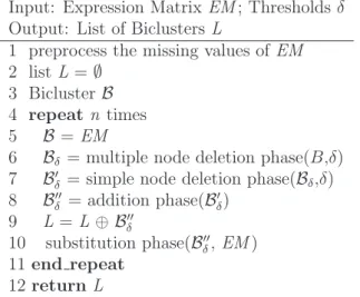
Fig. 1shows a scheme of CC. The algorithm takes as input the

expression matrix EMand the thresholddimposed on MSR.dis used to reject nond-biclusters. A listLofd-biclusters is returned as output. After preprocessing the missing values of the input data matrix by replacing them with random numbers, the bicluster dis-covering process is repeated as many times as biclusters are desired. In each iteration, the biclusterBis initialized to the whole matrix. Next, three different phases formultiple node deletion,single node deletion and node additionare applied. These phases itera-tively perform the removal and addition of rows and columns,

ensuring that the result is ad-bicluster. Finally, asubstitution phase

replaces the elements of the input matrix that are contained in the recently found bicluster with random values. This substitution is applied in order to prevent overlapping among biclusters, since it is very unlikely that elements covered by existing biclusters would contribute to any future bicluster. Although this strategy succeeds in avoiding the overlapping, CC presents several drawbacks due to this elements masking and also due to the use of a threshold for rejecting solutions, which is dependent on each dataset and must be computed before applying the algorithm.

3.1.3. SMSR-based biclustering (SMSR-CC)

A similar strategy to that of Cheng and Church has been adopted by Mukhopadhyay et al.[19]in order to incorporate their evalua-tion measure SMSR (Scaling MSR) into a search heuristics. SMSR is defined as follows: SMSRðBÞ ¼ 1 jIj jJj XjIj i¼1 XjJj j¼1 ðbiJbIjbijbIJÞ2 b2iJb 2 Ij ð3Þ

Note that SMSR is an adaptation of MSR able to recognize scal-ing patterns. Nevertheless, it is not capable to identify shiftscal-ing behaviors. As it is based on MSR, it also needs to initially set a limit value of SMSR for each dataset. Since SMSR is only able to recog-nize multiplicative models, the authors propose and adapted algo-rithm in which CC is applied twice, the fist time using MSR as evaluation measure and the second time using SMSR. Therefore, the strategy allows to independently find both types of patterns (shifting and scaling), but not simultaneously.

3.1.4. HARP algorithm

HARP (Hierarchical approach with Automatic Relevant dimension selection for Projected clustering) was presented by Yip et al.[20], and also introduced a new evaluation metric namedrelevance index

(RI). RI measures the quality of a bicluster as the sum of the rele-vance indices of the columns. Relerele-vance indexRIjfor columnj2J

is defined as: RIj¼1

r

2 Ij

r

2 j ð4Þ where

r

2

Ij(local variance) and

r

2j (global variance) are the variance

of the values in columnjfor the bicluster and the whole data set, respectively.

Iteratively, the biclusters are merged by choosing experimental conditions that satisfy a relevance index threshold. HARP maxi-mizes the quality when biclusters are constant, and its bottom-up merging strategy does not produce overlapped solutions.

3.1.5. Maximum Similarity Bicluster algorithm (MSB)

MSB was proposed by Liu and Wang[21]together with a simi-larity score for biclusters. The authors highlighted three different characteristics of their approach: (1) no discretization procedure is required, (2) MSB performs well for overlapping biclusters and (3) it works well for additive biclusters. This third property is a direct consequence of the use of the similarity score.

The algorithm starts with the whole matrix as the bicluster. Then a process of iteratively removing the row or column in the bicluster with the worst similarity score is performed, until there is one element left in the bicluster. During this process,nþm1 sub-matrices have been computed, wheren and mrefer to the number of rows and columns in the input matrix, respectively. MSB only outputs one bicluster, corresponding to the one in the

nþm1 sub-matrices with the maximum similarity score.

MSB works for the special case of approximately squared biclus-ters. In order to overcome this issue and also to speed up the pro-cess, an extension algorithm named RMSBE (Randomized MSB Extension algorithm) is also presented. RMSBE makes use of the average of the similarity scores between some pairs of genes in the bicluster, as well as of randomly selection to choose the refer-ence genes.

3.1.6. Weighted Fuzzy-Based Maximum Similarity Bicluster algorithm (WF-MSB)

Chen et al.[22]extended the MSB algorithm to propose a gen-eralized fuzzy-based approach, named WF-MSB (Weighted Fuzzy-based Maximum Similarity Biclustering), for extracting a query-driven bicluster based on the user-defined reference gene.

One of the advantages of this aproach is that WF-MSB discovers both of the most similar bicluster and the most dissimilar bicluster to the reference gene. Also, the expression values of the biclusters extracted by WF-MSB have high difference values compared to the baseline of all expression values, meaning that these biclusters are more significant.

3.1.7. Biclustering by Iteratively Sorting with Weighted Coefficients (BISWC)

In their approach, Teng and Chan [23] alternately sort and transpose the gene expression data, using weighted correlations at the same time to measure gene and condition similarities. The weighted correlation index is a variation ofPearson’s correlation coefficient, which was originally adapted by Bland and Altman

[24]in order to add weights when working with multiple observa-tions. In this work, Teng and Chan have redefined this index so that weights are assigned to the different features (genes or samples) according to their importance. This way, those features with more importance will have more impact than the others.

The algorithm is based on the dominant set approach of Pavan and Pelillo[25]. In order to find a bicluster, genes and conditions are iteratively sorted using weight vectors, which are also itera-tively refined using the sorting vector of the previous iteration. In each iteration the matrix is transposed and the process is repeated over the other dimension, thus alternating from genes to conditions. At the end of the process, the highly correlated bicluster is located at one corner of the rearranged gene expression data matrix, and is defined using a threshold for the correlation coefficients between adjacent rows and columns.

To find more than one bicluster, the authors use the weight vec-tors. This way, any time a bicluster is found, the weights of those features that have not been included in it are enhanced, at the same time as reducing the weights of those features included in it. Using this approach, overlapping among biclusters is permitted but controlled and penalized any time a gene or condition is included in a solution.

3.1.8. Biclustering by Correlated and Large Number of Individual Clustered seeds (BICLIC)

BICLIC[26]has been recently proposed as a biclustering algo-rithm based on the use ofPearson correlation coefficientfor biclus-ters evaluation. Regarding the search strategy, BICLIC is mainly made up of four different phases: finding biclusters seeds, expand-ing seeds, filterexpand-ing expansion products and checkexpand-ing and removexpand-ing duplicated biclusters.

The first phase produces an undetermined number of bicluster seeds by applying individual dimension-based clustering, where genes are labeled and merged according to their expression values in different conditions. These seeds are afterwards expanded in the second phase, where the expansion is performed in two ways: gene-wise and condition-wise, trying to merge each gene or condi-tion iteratively until a certain threshold over the average Pearson’s

correlation coefficient is exceeded. The products of the second phase are called candidate biclusters, and although not all genes may show correlated patterns over all conditions in a candidate bicluster matrix, it is ensured that all genes and conditions are cor-related with the seed bicluster. This way, in the third phase correlation-based biclusters are obtained by iteratively eliminating less correlated sets of genes and conditions. Nevertheless, different seed biclusters may converge to very overlapped correlation-based products. In order to eliminate duplicate already contained biclus-ters, a last phase is applied in which all biclusters are ordered in an increasing order of their sizes and compared. If every gene and condition in a certain bicluster is included in other bicluster, the smaller one is removed.

Although last phase of BICLIC checks for duplicated biclusters, no overlapping control strategy has been used in order to deter-mine or limit the amount of overlapped elements between biclusters.

3.1.9. Intensive Correlation Search (ICS)

Ahmed et al.[27]have more recently proposed a biclustering technique (ICS) together with a similarity measure for evaluating biclusters based on their shifting-and-scaling correlation (SSSim).

SSSim (Shifting and Scaling Similarity) is defined using local means of genes for a baseline (reference) condition pair, combined with and other condition pairs. The resulting score varies from 0 to 1 when evaluation pairs of genes, where a value of 1 indicates that both genes exhibit a perfect shifting-and-scaling correlation. In order to evaluate biclusters, two input parameter called

s

and

a

are used to consider correlations among genes and a partial or complete bicluster, respectively.

ICS (Intensive Correlation Search) strategy iteratively extract cor-related subspaces for different pairs of genes. These corcor-related sub-spaces correspond to maximal set of samples for which gene expressions are correlated by more than the user defined threshold

s

. Subspaces correspond to biclusters, which are initially formed by a pair of genes, being also iteratively extended to include more genes, until no more genes can be added to the bicluster. This extension phase is governed by the second user defined threshold,

a

. Initial gene pairs forming initial correlated subspaces must be formed by genes such that none of these are part of any bicluster that have been generated so far. Nevertheless, this constraint does not prevent genes to be part of several biclusters during the exten-sion phase, allowing thus overlapping among biclusters.

3.2. Stochastic iterative greedy search

Some authors have preferred using a stochastic strategy in order to add a random component to the iterative greedy search, rending thus the algorithm to be non-deterministic. Most impor-tant stochastic iterative greedy approaches are reviewed in this section.

3.2.1. Flexible Overlapped biClustering (FLOC)

Yang et al.[28]proposed a different heuristic for coping with the random masking of the values in the data matrix. To address this issue and to further accelerate the biclustering process, the authors presented a new model of bicluster to incorporate null val-ues. They also proposed an algorithm named FLOC (FLexible Overlapped biClustering) able to discover a set ofkpossibly overlap-ping biclusters simultaneously based on probabilistic moves.

The algorithm begins with the creation of k initial biclusters with rows and columns added to them according to a given prob-ability. After that, these biclusters are iteratively improved by the addition or removal of one row or column at a time, determining the action that better improves the average of the MSR values of the k biclusters. Bicluster volumes are also taken into account

within the possible actions, where bigger biclusters are preferred, and the variance is used to reject constant biclusters. The whole process ends when no action that improves the overall quality can be found.

3.2.2. Random Walk Biclustering (RWB)

Angiulli et al.[29]presented a biclustering algorithm based on a greedy technique enriched with a local search strategy to escape poor local minima. Their algorithm makes use of a gain function that combines three different objectives: MSR, gene variance and the size of the bicluster. These objectives are compensated by user-provided weights.

RWB produces one bicluster at a time. Starting with an initial random solution, it searches for a locally optimal solution by suc-cessive transformations that improve the gain function. A transfor-mation is done only if there is reduction of MSR or an increase either in the gene variance or the volume. In order to avoid getting trapped into poor local minima, the algorithm executes random moves according to a probability given by the user. To obtaink

biclusters RWB is executedk times by controlling the degree of overlapping among the solutions. This degree is controlled for genes and conditions independently by using two different fre-quency thresholds. This way, during any of the k executions of the algorithm, whenever a gene or condition exceeds the corre-sponding frequency threshold, it is removed from the matrix and therefore it will not be taken into account in the subsequent executions.

3.2.3. Reactive GRASP Biclustering (RGRASP-B)

GRASP is a multi-start meta-heuristics for combinatorial prob-lems, consisting of iterations made up of two phases: construction of a greedy randomized solution and local search in which its neighborhood is investigated until a local minimum is found. The best overall solution is kept as the result.Reactive GRASPis a vari-ant of GRASP in which the threshold parameter

a

associated to the candidate list of solutions is self-tuned, and its value is periodically modified according to the quality of the solutions recently obtained.

Dharan et al. [30] proposed a reactive GRASP biclustering method in which high quality bicluster seeds are generated using one-dimensionalk-means clustering. Afterwards, these seeds are further enlarged by adding more rows and columns to them, employing the reactive GRASP method, and also making use of ran-domized heuristics for escaping from local optima. The algorithm makes use of MSR score as the cost function to evaluate the quality of the obtained biclusters. In order to obtainkbiclusters,kseeds need to be generated in the first step, where their overlapping amount is controlled by the setting of the

a

values.

3.2.4. Pattern-Driven Neighborhood Search (PDNS)

Neighborhood search consists in iteratively improving an initial candidate solution by replacing it with a higher quality neighbor. It is usually obtained by performing little modifications on the for-mer one.

PDNS has been recently proposed by Ayadi et al. [31] as a

Pattern-Driven Neighborhood Searchapproach for the biclustering problem. Prior to the search, the method first applies a preprocess-ing step to transform the input data matrix into a behavior matrix

M00_{. Each row of this behavior matrix represents the trajectory}

pat-tern of a gene across all the combined conditions, while each col-umn represents the trajectory pattern of all the genes under a pair of particular conditions in the data matrix. M00 _{defines the}

problem search space as well as the neighborhoods used within the search process.

The initial bicluster is obtained by using two fast well-known greedy algorithms: CC and OPSM, and is encoded into its behavior matrix before being improved by PDNS. The algorithm alternates between two basic components: a descent-based improvement procedure and a perturbation operator. The descendent strategy is used to explore the neighborhood, moving to an improving solu-tion at each iterasolu-tion. This process is employed to discover locally optimal solutions. In order to displace the search to a new starting points, the perturbation operator is applied. It is carried out after the descent improvement stops according to one of two stopping criteria: the solution reaches a fixed quality threshold or a fixed number of iterations has been reached. A perturbed bicluster is then computed by a random replacement of 10 per cent of genes and conditions of the recorded best bicluster so far. This perturbed bicluster is used as a new starting point for the next round of the descent search, and the whole PDNS algorithm stops when the best bicluster is not updated for a fixed number of perturbations. For assessing the quality of two biclusters any time a replacement is taking place the ASR (Average Spearman’s Rho)[32], which is based on the use of theSpearman’s rank correlation.

The algorithm outputs one bicluster at a time. Therefore, in order to obtain several biclusters it must be run several times with different initial solutions. In this work, the authors use the output of two fast well-known algorithm as initial biclusters. Nevertheless, no overlapping control is carried out among the reported solutions.

3.3. Nature-inspired meta-heuristics

Nature-inspired meta-heuristics are characterized by reproduc-ing efficient behaviors observed in the nature. Examples of this kind of heuristics include evolutionary computation, artificial immune systems, ants colony optimization or swarm optimization, among others. All of them make use of algorithmic operators sim-ulating useful aspects of various natural phenomena and have been proven to be very effective for complex optimization problems. In this context, many biclustering approaches have been proposed based on the use of any of this kind of meta-heuristics, being evo-lutionary computation the most used. In the following, the most important biclustering approaches based on any nature-inspired meta-heuristics have been reviewed.

3.3.1. Simulated Annealing Biclustering (SA-B)

Simulated Annealing(SA) stochastic technique originally devel-oped to model the natural process of crystallization and has been adopted to solve optimization problems[33]. SA algorithm itera-tively replaces the current solution by a neighbor one if accepted, according to a probability that depends on both the fitness differ-ence and a global parameter called the temperature. This temper-ature is gradually decreased during the process, decreasing the probability of randomly choosing the new solution when it gets lower.

The specific behavior of any simulated annealing approach is mainly given by the fitness function an the depth of the search at each temperature. In Bryan et al.[34]approach, the fitness of each solution is given by its MSR value, and ten times the number of genes successes needed to be achieved before cooling. This number determines the depth of the search, being a success an improve-ment on the fitness function. The initial temperature of the system, as well as the rate at which it is lowered are also important, since both of them determine the number of total iterations and also affect the convergence. The authors set them experimentally.

The algorithm must be runktimes in order to obtaink biclus-ters. Solutions are masked in the original matrix in order to avoid overlap among them. In their work, Bryan et al. used the same method of Cheng and Church [12], replacing the original values

with random ones, in an attempt to prevent them to be part of any further bicluster.

3.3.2. Crowding distance based Multi-Objective Particle Swarm Optimization Biclustering (CMOPSOB)

Particle Swarm Optimization (PSO) technique simulates the social behavior of a flock of birds or school of fishes which aim to find food. The system is initialized with a population of random solutions and searches for optima by updating generations. Potential solutions are called particles and fly through the problem space by following the current optimum. Particles have memory for retaining part of their previous state, and decide the next move-ment influenced by randomly weighted factors affecting the best particle previous position and the best neighborhood previous position. The global optimal solution is the best location obtained so far by any particle in the population and the process ends when each particle reaches its local, neighborhood and global best positions.

Liu et al.[35]based their biclustering approach on the use of a PSO together with crowding distance as the nearest neighbor search strategy, which speeds up the convergence to the Pareto front and also guarantees diversity of solutions. Three different objectives are used in CMOPSOB: the bicluster size, gene variance and MSR, which have been incorporated into a multi-objective environment based on the individuals dominance. Being a popula-tional approach, several potential solutions are taken into account in each generation. Those non-dominated solutions in the last gen-eration will be reported as the output.

3.3.3. Multi-Objective Multi-population artificial immune Network (MOM-aiNet)

Inspired by biological immune systems, Artificial Immune Systems (AIS) have emerged as computational paradigms that apply immunological principles to problem solving in a wide range of areas. Coelho et al.[36] presented an immune-inspired algo-rithm for biclustering based on the concepts of clonal selection and immune network theories adopted in the original aiNet algorithm by Castro and Von Zuben[37]. It is basically con-stituted by sequences of cloning, mutation, selection and suppres-sion steps.

MOM-aiNet explores a multi-population aspect, by evolving several sub-populations that will be stimulated to explore distinct regions of the search space. After an initialization procedure con-sisting on random individuals made up of just one row and one col-umn, populations are evolved by cloning and mutating their individuals. The authors apply three different kind of mutations: insert one row, insert one column or remove one element, either row or column. They only consider two different objectives: MSR and the volume, using the dominance among individuals in order to replace individuals with higher quality ones. A suppression step is periodically performed for the removal of individuals with high affinity (overlap), causing thus fluctuations in the populations sizes. Nevertheless, this step is followed by an insertion one, in which new individuals are created, giving preference to those rows or columns that do not belong to any bicluster. After a predefined number of iterations, MOM-aiNet returns all the non-dominated individuals within each sub-population.

3.3.4. Evolutionary algorithms for biclustering

Evolutionary algorithmsare based on the theory of evolution and natural selection. Being the oldest of the nature-inspired meta-heuristics, they have been broadly applied to solve problems in many fields of engineering and science. Many biclustering approaches have been proposed based on evolutionary algorithms. Being a populational approach, a larger subset of the whole space of solutions is explored, at the same time that it helps them to

avoid becoming trapped at a local optimum. These reasons make evolutionary algorithms very suited to the biclustering problem.

Starting by an initial population, evolutionary algorithms select some individuals and recombine them to generate a new popula-tion of individuals. This process is repeated for a number of gener-ations until the algorithm converges or certain criterion is met. A general scheme of an EA is presented inFig. 2. Given a certain prob-lem that defines a search space (sets of possible biclusters in this context), the EA starts by generating the initial population, that is the initial set of candidate solutions (line 1). These individuals are evaluated (line 2) using problem-dependent metrics which provide a fitness (/) for each candidate solution. Subsequently, off-spring is produced by evolving the existing solutions, where fittest solutions often have a higher probability of being selected for reproduction. Thus, the population evolves in the iterative process (lines 3–9), by obtaining the new population based on the current population (P) and the intermediate population (P00_{) generated by}

applying the selection function and the genetic operators (cross-over and mutarion). Stopping criteria is usually related to a signif-icant improvement on the solutions through generations combined with a maximum number of iterations. Finally, the best solution or set of solutions of the las population are returned.

Next, we summarize the most relevant biclustering approaches based on evolutionary algorithms, both single or multi-objective. Although the majority of them aim at optimizing the popular met-ric residue (MSR), some of them are also based on correlation coefficients.

Bleuler et al.[38] (Bleuler-B) were the first in developing an evolutionary biclustering algorithm. They proposed the use of bin-ary strings for the individuals representation, and an initialization of random solutions uniformly distributed according to their sizes. Bit mutation and uniform crossover are used as reproduction oper-ators, and a fitness function that prioritises MSR. For those solu-tions with MSR below the thresholdd, bigger bicluster sizes are preferred. Tournament has been used as selection mechanism, where populations are completely replaced with new offspring. A diversity maintenance strategy is carried out which decreases the amount of overlapping among bicluster, and CC algorithm is also applied as a local search mainly to increase the size of the individ-uals. At the end, the whole population of individuals is returned as the set of quality biclusters.

SEBI was presented by Divina and Aguilar-Ruiz [14] as a

Sequential Evolutionary BIclusteringapproach. The term sequential refers the way in which bicluster are discovered, being only one bicluster obtained per each run of the evolutionary algorithm. In order to obtain several biclusters, a sequential strategy is adopted, invoking the evolutionary process several times. Furthermore, a

matrix of weights is used for the control of overlapped elements among the different solutions. This weight matrix is initialized with zero values and is updated every time a bicluster is returned. Individuals consists of bit strings, and are initialized randomly but containing just one element. Together with tournament selection, three different crossover and mutation operators are used with equal probability in reproduction: one-point, two-points and uni-form crossovers, and mutations that respectively add a row or a column to the bicluster or the standard mutation. Elitism is also applied in order to preserve the best individual through genera-tions. Individual evaluations are carried out by a single fitness function in which four different objectives have been put together: MSR, row variance, bicluster size and an overlapping penalty based on the weight matrix.

BiHEA (Biclustering via a Hybrid Evolutionary Algorithm) was pro-posed by Gallo et al. [39]and is very similar to the evolutionary biclustering algorithm of Bleuler et al. Both of them perform a local search based on CC algorithm, and return the set of individuals in the last population as the output. However, they differ in the cross-over operator (BiHEA uses two-point crosscross-over) and BiHEA also incorporates gene variance in the fitness function. Furthermore, two additional mechanisms are also added in order to improve the quality of the solutions. The first one is elitism, in which a pre-defined number of best biclusters are directly passed to next gen-eration, with the sole condition that they do not get over a certain amount of overlap. The second one makes use of an external archive to keep the best generated biclusters through the entire evolutionary process, trying to avoid the misplacement of good solutions through generations.

Huang et al.[40]have proposed a new biclustering algorithm based on the use of an EA together with hierarchical clustering. The authors argue that with such a huge search space, the EA itself should not be able to find optimal or approximately optimal solu-tions within a reasonable time. Therefore, they propose to separate the conditions into a number of conditions subsets, also called sub-spaces. The evolutionary algorithm is then applied to each subspace in parallel, and a expanding and merging phase is finally employed to combine the subspaces results into the output biclusters. As it is related only to the condition dimension, the EA is called CBEB, from

Condition-Based Evolutionary Biclustering, where the normalized geometric selection method is used as the selection function and the simple crossover and binary mutation methods are employed for reproducing the offspring. In both CBEB and the expanding and merging phase MSR score has been used for the evaluation of the potential solutions, always using the predefined threshold

das the upper limit.

More recently, Evo-Bexpa (Evolutionary Biclustering based in Expression Patterns)[41]has been presented as the first bicluster-ing algorithm in which it is possible to particularize several biclus-ter features in biclus-terms of different objectives. This way, if any previous information related to the microarray under study is available, the search can be guided towards the preferred types of biclusters (number of genes and conditions, overlapping amount or gene variance). These objectives have been put together by using a single Aggregate Objective Function (AOF). Furthermore, other objectives defined by the user can also be easily incorporated into the search, as well as any objective may be ignored. Furthermore, Evo-Bexpa bases the bicluster evaluation in the use of expression patterns, making use of the VEt_{metric, able to find}

shifting and scaling patterns in biclusters, even simultaneously.

3.3.5. Multi-objective evolutionary algorithms

Apart from the specific homogeneity measure for biclusters, many authors have also incorporated other objectives to the search, such as the bicluster volume or gene variance. These requirements are often conflicting. For example, the bigger a

bicluster is, the more probable to have a higher MSR value. Nevertheless, bigger biclusters with low MSR values are preferred. The four EA approaches review above make use of a single aggre-gate objective function which combines the different objectives. In this section we review those EA approaches that optimize the different objectives according to other multi-objectives schemes.

In the work of Mitra and Banka[42](M&B), the first approach that implements a Multi-Objective EA (MOEA) based on Pareto dominance is presented. The authors base their work on the NSGA-II [43], and look for biclusters with maximum size and MSR value, as long as it is smaller than the upper boundd. Also, a local search strategy based on thenode insertionandnode deletion

phases of CC algorithm is applied to all of the individuals at the beginning of every generational loop. Populations are ranked according to the dominance criterion, crowding tournament selec-tion is performed, the selected individuals are crossed and mutated, and the best individuals among the new and old popula-tions are selected to remain in the next generation.

In MOGAB (Multi-Objective GA-based Biclustering algorithm)[44], the authors propose the use of a new individual representation, encoded as strings made up of two parts: in the first one, indexes of genes acting as cluster centers of sets of genes are represented, while the second one keeps the indexes of the conditions acting as cluster centers of sets of conditions. This way, each individual does not represent a bicluster, but a set of biclusters, obtained with the different possible combinations of clusters of genes and conditions. The initial population contains randomly generated individuals, where each gene or condition is equally probable to become the center for a gene or a condition cluster, respectively. MOGAB is also based on the NSGA-II strategy, and performs crowded binary tour-nament selection, single-point crossover and standard mutation, although these two last operators are carried out on gene and con-dition centers strings independently, and invalid individuals are marked when appear in order not to let them reproduce in the next generation. Elitism has also been incorporated in MOGAB to track the non-dominated Pareto-optimal solutions. Within the evalua-tion, MSR and row variances are computed for all thedbiclusters denoted by each individual. A fitness vector is afterwards created with the mean of their fitness. From the non-dominated individu-als in the final population, all thedbiclusters are extracted and output as the final biclusters.

Since the boundaries of biclusters usually overlap, some authors believe the notion of fuzzy sets is useful for discovering such over-lapping biclusters. In this regard, a fuzzy version of MOGAB, named MOFB(Multi-Objective Fuzzy Biclustering algorithm) is proposed in

[45]. MOFB simultaneously optimizes fuzzy versions of MSR, row variance and volume and applies a interesting variable string length encoding scheme.

SMOB (Sequential Multi-Objective Biclustering) has been used together with different measures, such as MSR and VE (Virtual Error[46]) by Divina et al., adopting a sequential strategy similar to SEBI[14]. Unlike SEBI, where a single-objective EA was used, SMOB invokes a multi-objective evolutionary algorithm (MOEA) several times. Each time the MOEA is called, a bicluster is returned and stored in a list. The number of elements in the output list rep-resents the number of found solutions. In these works, biclusters with high volume, good quality (being quality measured by an appropriate metric such as VE, MSA or MSR) and relatively high gene variance are addressed. Thus, three objectives have been indi-viduated to be optimized, being in conflict with each other.

3.4. Clustering-based approaches

This section describes those biclustering algorithms which base their search on the use of a traditional one-dimension clustering

algorithm, together with an additional strategy providing the sec-ond dimention analysis.

3.4.1. SVD and clustering-based approaches

Possibilistic Spectral Biclustering (PSB). A biclustering approach based on the use of Singular Value Decomposition

(SVD) together with one-dimensional clustering named PSB was proposed by Cano et al.[47]. The use of SVD techniques enhances the clustering process by performing dimensionality reduction.

This algorithm consists of firstly applying SVD method on an eigenproblem formulated on the input matrix and get minðn;mÞsolution eigenvectors, wherenandmrefers to the number of genes and conditions in the input matrix. Using these eigenvectors several partition matrices are created. Two inde-pendent clustering algorithms are then executed on them: for those rows representing genes and for those representing con-ditions in the original matrix, respectively. Each combination of a cluster of genes and a cluster of conditions is a candidate bicluster, which will be post-processed in order to improve its quality when possible, or rejected if it is not considered a qual-ity solution. Finally, the whole process is repeated with a linear inversion of the input expression matrix, in order to also obtain under-expressed genes.

The clustering algorithm used in PSB is a variation of the

Improved Possibilistic Clustering(IPC) by Zhang and Leung[48], which mixes possibilistic and probabilistic approaches. MSR is used at both the clustering and the crisping of the possibilistic biclusters, though in this last step the volume is also taken into account. Possibilistic clustering allows a considerable amount of overlapping, so the authors have also added to the process an overlapping control, in which a bicluster is checked for its over-lapping amount before being added to the result set.

Biclustering with SVD and Hierarchical Clustering (SVD&HC-B).Yang et al.[49]have recently proposed a strategy similar to the one of Cano et al.[47], by usingSingular Value Decomposition(SVD) together with clustering and a final stage to merge and filter the clusters. In this approach, the authors make use of thesub-matrix correlation scorealso presented in their work. A upper bounddis used to defined adcorbicluster as a bicluster with a sub-matrix correlation score lower thand. In a first step, two different matrices namedRðlÞ_{(a group of basis}

genes) and CðlÞ _{(a group of basis conditions) are obtained by}

using SVD. Secondly, after centralizing the rows of these two matrices, clustering is applied to both of them by theMixed Clustering algorithm, based on agglomerative hierarchical clus-tering and on the use of the sub-matrix correlation score as dis-similarity measure. The number of clusters produced by this technique is not known beforehand. This way, a set ofmand

ngroups of clusters are obtained from both matrices. Every pair of these groups constructs a bicluster, obtainingmn biclus-ters in this way. Nevertheless, not every pair of groups may be adcorbicluster, and a final step is executed in order to obtain inclusion-maximal biclusters. This last step is carried out by the Lift algorithm, inspired in the node-deletion and

node-addition phases proposed by Cheng and Church, but according to the sub-matrix correlation score. Since the cluster-ing algorithm generates not mutually exclusive clusters, the biclusters obtained by this method are possible overlapped.

3.4.2. Biclustering based on Related Genes and Conditions Extraction (RGCE-B)

Yan et al. [50] have recently proposed a search strategy for obtaining biclusters with related genes and conditions of a given

bicluster type. They apply hierarchical clustering to different data matrices generated from the input one, according to genes/condi-tions stability and different bicluster types. Additionally, as a pre-processing step, missing data is estimated with the James–Stein method and Kernel estimation principle, where k means is used to obtain the estimation matrix.

Stable and unstable genes/conditions are first selected base on the cosine of the angle between the vector x¼ ð1;1;. . .;1Þand each row/column of the data matrix. This way, and using a prede-fined threshold, those vectors more similar toxare considered to be stable, and unstable otherwise. Using this criterion, the gene expression matrix can be partitioned to submatrices of stable and unstable ones in both the row and column directions.

On the other hand, five different types of biclusters previously defined in the literature have been used (see Section2.1): C (con-stant values), CR (con(con-stant values on rows), CC (con(con-stant values on conditions), ACV (additive coherent values) and MCV (multiplica-tive coherent values). Using these definitions it is possible to state that C and CR types exist in row-stable matrices, C and CC types exist in column-stable matrices, while ACV and MCV types exist in unstable matrices.

The process therefore consist in the creation of a sparse matrix with the same size as that of the original gene expression matrix for each type of biclusters, where the zero and non-zero entries correspond to the irrelative and related genes and conditions, respectively. After reducing the dimension of these matrices, biclusters of any type can be obtained based on the corresponding sparse matrix. In this approach, a hierarchical agglomerative single linkage method is used to perform clustering in both the row and column directions, for each sparse matrix. Biclusters are afterwards obtained by finding the overlapping parts between clusters in dif-ferent directions. As a final post-processsing step, bicluters are refined by deleting rows and columns according to a MSR threshold.

4. Non metric-based biclustering

In this section we review the most important biclustering approaches that exclude the use of any evaluation measure for guiding the search. We have classified them according to their most relevant aspects: specific algorithm, data structure represen-tation or the main important basis. Likewise that in Section3, it is important to note that different categories are not exclusive, that is, the algorithms have been grouped attending to what we have considered to be their most distinctive property, althougth some of them may as well be assigned to more than one group.

4.1. Graph-based approaches

This section reviews four different biclustering approaches based on the use of graph theory. Some of them use nodes for bicluster elements representation, either genes, samples or both genes and samples, while some other make use of nodes for repre-senting whole biclusters.

4.1.1. SAMBA

Tanay et al.[13]based their approach on graph theoretic cou-pled with statistical modeling of the data, where SAMBA stands for Statistical-Algorithmic Method for Bicluster Analysis. In their work, they model the input expression data as a bipartite graph whose two parts correspond to conditions and genes, respectively, and edges refer to significant expression changes. The vertex pairs in the graph are assigned weights according to a probabilistic model, so that heavy sub-graphs correspond to biclusters with high likelihood. Furthermore, they present two statistical models of the

resulting graph, the second one being a refined version of the first in order to include the direction of expression change, allowing thus to detect either up or down regulation. Weights are assigned to the vertex pairs according to each model so that heavy sub-graphs correspond to significant biclusters. This way, discover-ing the most significant biclusters means finddiscover-ing the heaviest sub-graphs in the bipartite graph model, where the weight of a sub-graph is the sum of the weights of the gene-condition pairs in it. In order to cope with noisy data, Tanay et al. searched for sub-graphs that are not necessarily complete, assigning negative weights to non-edges.

In order to reduce the complexity of the problem, high-degree genes are filtered out, depending on a pre-defined threshold. According to the authors, the number of genes is reduced by around 20 per cent, considering it to be a modest reduction. The proposed algorithm is an iterative polynomial approach based on the procedure for solving the maximum bounded bi-clique prob-lem, where a hash-table is used for the identification the heaviest bi-clique. A generalization of this method is applied in order to give the k heaviest non-redundant sub-graphs, where k is an input parameter. Before applying the algorithm, the graph structure may be created, using the signed or unsigned model depending on the input data.

4.1.2. MicroCluster

MicroCluster was developed by Zhao and Zaki[51]as a biclus-tering method for mining maximal biclusters satisfying certain homogeneity criteria, with possible overlapped regions. Biclusters with shifting patterns are detected by using exponential transfor-mations. Furthermore, by means of these kind of transformations, scaling patterns may also be detected.

MicroCluster uses an enumeration method consisting of three steps. Firstly, a weighted, directed range multi-graph is created for representing the possible valid ratio ranges among experimen-tal conditions and the genes that meet those ranges. A valid ratio range is an interval of ratio values satisfying several constraints on expression values. In this graph, vertices correspond to samples and each edge has an associated gene set corresponding to the range on that edge. The construction of this range multi-graph fil-ters out most unrelated data. Once the multi-graph is created, a second step is applied for mining the maximal clusters from it, based on a recursive depth-first search. Although the output of this step is the final set of biclusters, a final step is optionally executed in order to delete or merge those biclusters according to several overlap conditions. This last step is also applied to deal with noise in data, controlling the noise tolerance.

4.1.3. QUBIC

QUBIC has been presented as aQUalitative BIClustering algorithm

[52], in which the input data matrix is first represented as a matrix of integer values, either in a qualitative or semi-qualitative man-ner. In this representation, two genes are considered to be corre-lated under a subset of conditions if the corresponding integer values along the two corresponding rows of the matrix are identi-cal. The qualitative (or semi-qualitative) representation is such that allows the algorithm to detect different kind of biclusters, also including scaling patterns. It is also suitable for finding both posi-tively and negaposi-tively correlated expression patterns, where nega-tive correlations will be represented by opposite signs across the entire row. The biclustering problem consist now in finding all the optimal correlated sub-matrices.

The first step of the algorithm correspond to the construction of a weighted graph from the qualitative or semi-qualitative matrix, with genes represented as vertices, and edges connecting every pair of genes. Edge weights are computed in the base of the simi-larity level between the two corresponding rows. After the graph

has been created, biclusters are identified one by one, starting for each bicluster with the heaviest unused edge as a seed. This seed is used to build an initial bicluster and the algorithm iteratively adds additional genes into the current solution. The consistency level marks the end of the search for a bicluster, since it determines the minimum ratio between the number of identical non-zero inte-gers in a column and the total number of rows in the sub-matrix.

4.1.4. CoBi

CoBi (Pattern-based Co-Regulated Biclustering of Gene Expression Data)[53]makes use of a tree to group, expand and merge genes according to their expression patterns. In order to group genes in the tree, a pattern similarity between two genes is defined given their degrees of fluctuation and regulation patterns. While the first is used to represent the expression levels variations among condi-tions,the regulation pattern represents the up, down and no regu-lation. this way, CoBi is able to find biclusters exhibing both positive and negative regulation among genes.

The process consist of generating biclusters by means of a tree with a single pass of the dataset. After preprocessing the input data, computing both the degrees of fluctuation and the regulation patterns, CoBi starts by creating an initial BiClust tree. This tree will containM1 initial nodes, whereMis the number of exper-imental conditions in the datasets. The first step corresponds to the creating of leaf nodes for each branch of the tree, by forming clus-ters of genes based on the previously defined similarity. To main-tain a moderate number of gene clusters a pruning step is performed, where a cluster is removed if its size is below a certain threshold. Next, in the second phase, the tree is iteratively expanded and merged to produce higher order biclusters. The merging is carried out in two different ways: at a non-leaf level and at a cluster level. Since this merging phase might produce clus-ters already contained in the same branch, they will be identified and removed from the tree. Once the tree reaches the end of expansion so that no further merging is possible, CoBi returns the list of all non-redundant obtained biclusters.

4.2. One-way clustering-based approaches

Similar to Section3.4regarding non metric-based biclustering approaches, this section describes those biclustering algorithms which base their search on the use of a traditional one-dimension clustering algorithm, together with an additional strategy providing the second dimention analysis. In this case, the algorithms reviews do not make use of any bicluster evaluation measures within the search.

4.2.1. Coupled Two-way Clustering (CTWC)

Coupled Two-Way clustering(CTWC), introduced by Getz et al.

[54] defines a generic scheme for transforming a one-dimensional clustering algorithm into a biclustering algorithm. They define a bicluster as a pair of subsets of genes and conditions, or a pair of gene and conditions clusters. They also define a stable cluster as a cluster that is statistically significant according to some criterion (such as stability, critical size, or the criterion used by Hartigan[55]). Getz et al. also applied a normalization step based on euclidean distance as a previous step to the application of the algorithm.

The heuristics provided by CTWC consists in an iterative pro-cess restricting the possible candidates for the subsets of genes and samples, only considering and testing those genes and samples clusters previously identified as stable clusters. The iterative pro-cess is initialized with the full matrix. Both sets of genes and sam-ples are used to perform two-way clustering, storing the resulting stable clusters in one of two registers of stable clusters (for genes or samples). Pointers that identify parent clusters are also stored,

consisting thus in a hierarchical approach. These steps are iterated further, using pairs of all previously found clusters, and making sure that every pair is treated only once. The process is finished when no new clusters that satisfy the criteria are found.

The success of this strategy depends on the performance of the one-dimensional clustering algorithm. According to the authors, CTWC can be performed with any clustering algorithm. Nevertheless, many popular clustering algorithms (e.g. K-means, Hierarchical, SOM) cannot be used in this approach, since they do not readily distinguish significant clusters from non-significant clusters or make a priori assumption on the number of clusters [13]. Getz et al. [54] recommend the use of the SPC (superparamagnetic clustering algorithm)[56], which is especially suitable for gene microarray data analysis due to its robustness against noise and its ability to identify stable clusters.

4.2.2. Interrelated Two-way Clustering (ITWC)

Interrelated Two-Way Clustering(ITWC) developed by Tang and Zhang[57]is an algorithm similar to CTWC, combining the results of one-way clustering on both dimensions separately. A pre-processing step based on row normalization is also applied, where rows with little variation are removed from the input matrix. Although correlation coefficient is used as similarity mea-sure to meamea-sure the strength of the linear relationship between two rows or two columns in the process, Tang and Zhang do not propose any quality metric for the evaluation of a sub-matrix as a whole. For this reason we have categorized this approach as a non-metric based.

The idea behind ITWC is to discover the relationships between gene and sample clusters while iteratively clustering through both dimensions to extract important genes and classify samples simul-taneously. Within each iteration there are five main steps. First step performs clustering on rows, while in the second step cluster-ing is performed in the column dimension, for each group of genes from step one. In this second step, only two clusters are obtained for each gene group. Third step combines the former steps results by computing diverse sets intersections for the sample groups, resulting in 2k _{sample groups, where k is the number of gene}

clusters obtained in step one. Fourth step aims at finding heteroge-neous groups of conditions (which do not share rows used for clus-tering), being the result of this step a set of highly disjoint biclusters. Last step of ITWC sorts the rows in descending order of the cosine distance between each row and a row representative of each bicluster. After that, only the first one third of rows is kept, reducing thus the row set for each heterogeneous group. A likeli-hood based on the correlation coefficient is calculated for each heterogeneous group, being the reduced genes of the group with the higher likelihood value the selected for the next iteration. These genes and the entire samples then form a new gene expres-sion matrix from which a new iteration starts. Iterations will be terminated when a stable and significant pattern of samples has emerged. For this purpose, the authors use a criterion based on a coefficient of variation to measure how internally-similar and well-separated the partition is.

Biclusters identified by ITWC have no elements in common, due to the search strategy. This way, overlapping among biclusters is not allowed in this approach.

4.3. Probabilistic models

A probabilistic model is a model created using statistical analysis to describe data based on the use of probability theory. In this section, we review those algorithms which look for biclus-ters in a dataset making use of different types of probabilistic models.