Neural Network Methods for Nonparametric Probabilistic Forecasting

(1)

Lehigh University

Lehigh Preserve

Theses and Dissertations

2019

Neural Network Methods for Nonparametric

Probabilistic Forecasting

Konstantinos Miltiadis Hatalis

Lehigh University

Follow this and additional works at:https://preserve.lehigh.edu/etd Part of theElectrical and Computer Engineering Commons

This Dissertation is brought to you for free and open access by Lehigh Preserve. It has been accepted for inclusion in Theses and Dissertations by an

Recommended Citation

Hatalis, Konstantinos Miltiadis, "Neural Network Methods for Nonparametric Probabilistic Forecasting" (2019).Theses and Dissertations. 5563.

(2)

NEURAL NETWORK METHODS FOR

NONPARAMETRIC PROBABILISTIC

FORECASTING

by

KONSTANTINOS MILTIADIS HATALIS

Presented to the Graduate and Research Committee of Lehigh University

in Candidacy for the Degree of Doctor of Philosophy

in

Electrical Engineering

Lehigh University May, 2019

(3)

c

(4)

Approved and recommended for acceptance as a dissertation in partial fulfill-ment of the requirefulfill-ments for the degree of Doctor of Philosophy.

Date

Accepted Date

Dissertation Advisor

Committee Members:

Prof. Shalinee Kishore (Committee Chair)

Prof. Parv Venkitasubramaniam

Prof. Wenxin Liu

(5)

Acknowledgments

The completion of this Ph.D. is the culmination of immense hard work. Not only from myself, but also from everyone around me in my life in pushing and inspiring me to complete it. Although I just mention a few individuals here, I am deeply appreciative of everyone who has helped me along the way.

Firstly, I would like to express my enormous gratitude to my advisor Prof. Sha-linee Kishore for the continuous support of my Ph.D. research, for her patience, motivation, and immense knowledge. I am grateful to her for giving me the chance to join her lab group and for allowing me to pursue my research passion in machine learning. I could not have imagined having a better advisor and mentor for my Ph.D. study. Along with my advisor, I would like to thank the rest of my dissertation com-mittee: Prof. Parv Venkitasubramaniam, Prof. Wenxin Liu, and Prof. Alberto J. Lamadrid, for their insightful comments, reviews of my papers, and remarks. Most importantly they all pushed me with hard questions which motivated me to widen my research from various perspectives. I also want to give special thanks to all the anonymous reviewers, editors, and publishers of all my papers.

My sincere gratitude also goes to Prof. Rick S. Blum, Prof. Larry Snyder, Prof. Arindam Banerjee, and Prof. Katya Scheinberg, who at different times of my Ph.D. provided me with valuable feedback on my research. Thanks also go to the staff of Lehigh: Ruby Scott, Diane Hubinsky, Brie Lisk, and David Morrisette. I thank my fellow labmates, in Prof. Kishore’s group, Dr. Parth Pradhan and Dr. Kwami Senam Sedzro. In all the years we spent together, in our shared office space in PA 401, I very much enjoyed our stimulating discussions and all the fun we had together. Kwami, your life stories continue to inspire me, and Parth your comradeship working

(6)

together side by side was remarkable. I want to give big thanks to my fellow doctoral student, and one of my closest friends, Dr. Dustin Dannenhauer. I’ll never forget our amazing discussions and ideas on AI, our epic Go and Starcraft game nights, and all the veggie burgers we ate together.

I give the biggest thanks to my family who all have given me unconditional support. To my sisters Maria and Amalia, they have been my life long friends. To my mother, whom I am so gracious for everything you have done for me. And to my fianc´ee, future wife, best friend, and soulmate Radhika. Your understanding, encouragement, and love have kept me going through all the late nights and long hours. Finally, I would like to dedicate this dissertation to my father, Prof. Miltiadis Hatalis. My father is the sole inspiration to go into graduate school and pursue a Ph.D. in engineering. His guidance throughout high school, college, and graduate school have elevated me to success.

(7)

List of Tables

2.1 Table of error statistics with minor noisy data. . . 34

2.2 Table of error statistics with higher noisy data. . . 35

3.1 Simulation parameters used in case studies. . . 56

3.2 Evaluation metrics for attack detection. . . 71

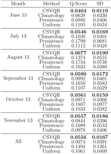
4.1 Results of prediction interval reliability in different months. . . 86

4.2 Summary of the mean Q-score across all quantiles for a given method and month and their standard deviation. . . 87

6.1 Datasets used in the experiments. . . 131

6.2 Hyperparameters estimated by grid search for ARIMA and SARIMA for each case study. The seasonal term S is estimated using the ACF plot. . . 132

6.3 Quantiles scores from QFNN and benchmark methods. . . 132

(12)

List of Figures

1.1 Reading order of the dissertation. . . 14

2.1 Example of a NARX network. . . 19

2.2 NAR network series mode. . . 22

2.3 NAX network parallel mode. . . 22

2.4 The scheme for value of the inertia weight w. . . 24

2.5 PSONAR learning algorithm. . . 27

2.6 3D plot of spatial distribution of simulated ocean waves. . . 28

2.7 Training data window sample of 30 seconds. . . 28

2.8 10 second lookahead (20 steps) PSONAR prediction example. . . 29

2.9 10 second lookahead (20 steps) NARNET prediction example. . . 31

2.10 Convergence plot of PSONAR in Fig. 2.8. . . 33

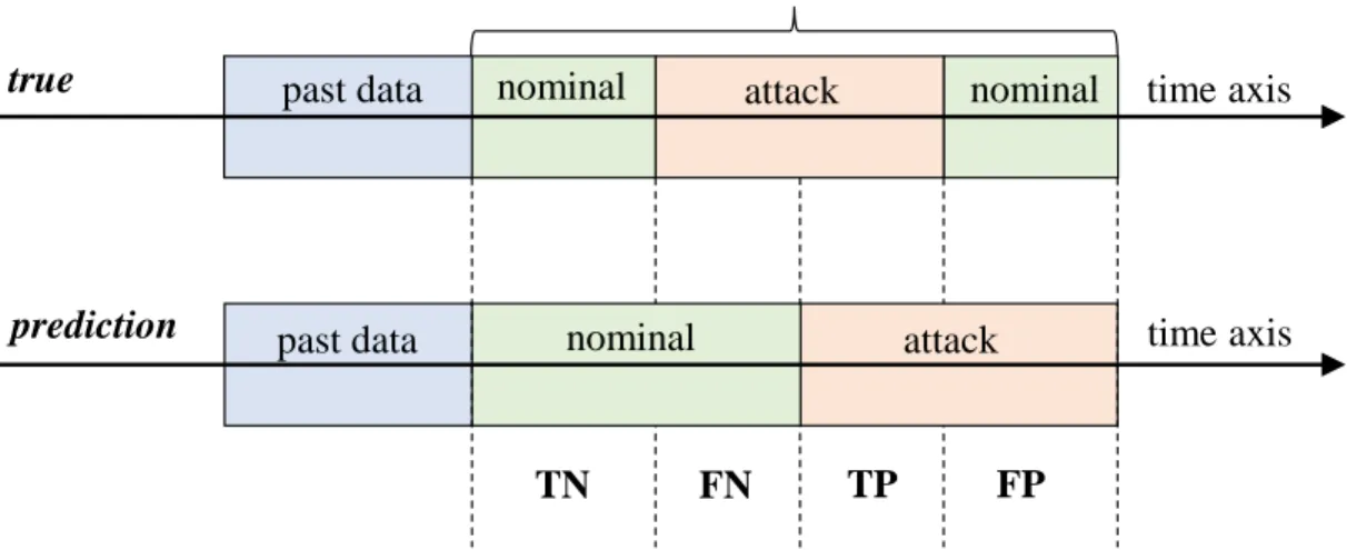
3.1 Feedback effect between price and DSM demand. As prices go up, demand decreases. But if prices are hijacked and false prices are fed to DSM systems then a false low price increases demand, and a false high price can decrease demand. The same is true if demand was altered by an attack. If load usage is increased by an attacker then prices would increase and vice versa. . . 40

3.2 Various demand side management goals. . . 43

3.3 Process of block bootstrap simulation of a new home power usage (bottom) from a template home (top). Example simulation samples are taken from four days from the template series with replacement. . 49

(13)

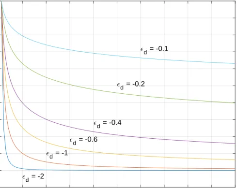
3.4 Load as a function of price with arbitrary price range $1-100, α = 10,000, and d= -0.1,-0.2,-0.4,-0.6,-1, -2. . . 51

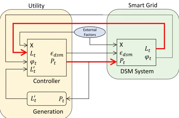
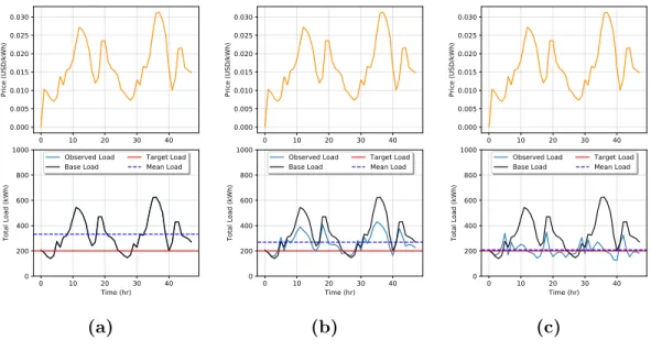
3.5 Block diagram highlighting the feedback between the utility and grid. 55 3.6 Simulation of price-load interaction with Goal 1 with DSM when

κi = 0,∀i (a), κi = 0.5,∀i (b), and κi = 0.99,∀i in (c). . . 56

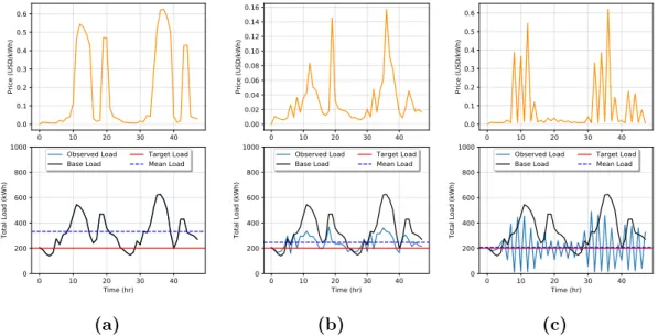
3.7 Simulation of price-load interaction with Goal 2 with DSM when

κi = 0,∀i (a), κi = 0.5,∀i (b), and κi = 0.99,∀i in (c). . . 57

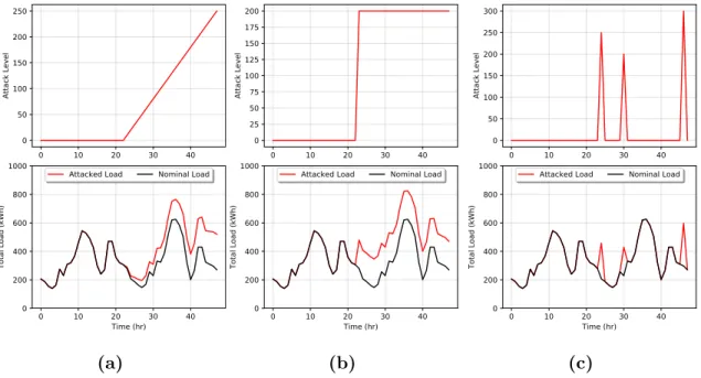
3.8 Examples of different type of DSM attacks: (a) ramp attack, (b) sudden attack, and (c) point attack. . . 59 3.9 Confusion matrix imposed on a time axis of attack predictions vs true

observations. . . 60 3.10 ACF and PACF fplots of the residual series between the SARIMA fit

tp training data. From the plots we observe that the residuals are stationary. . . 62 3.11 Q-Q plot of the residual series between the SARIMA fit tp

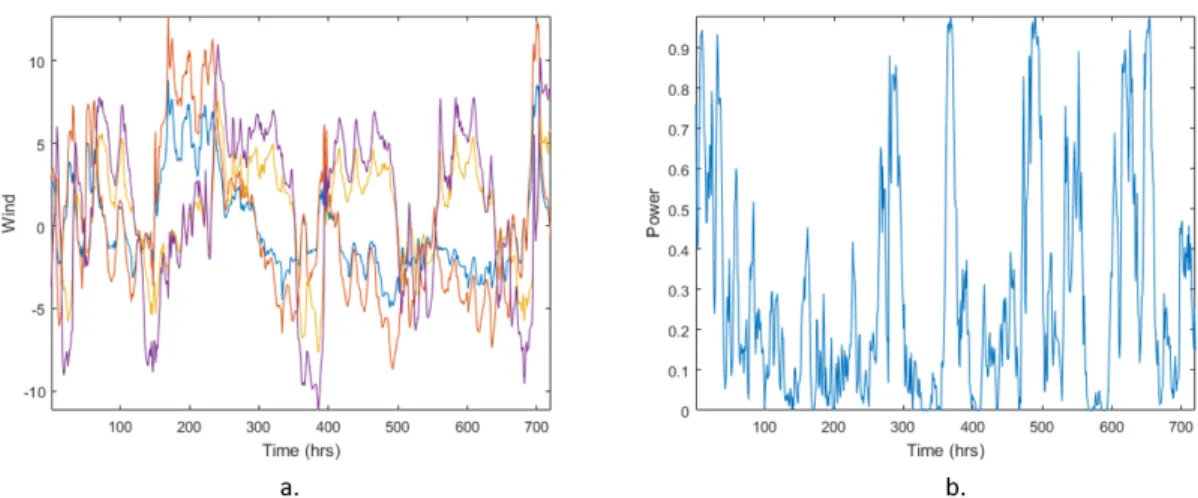
train-ing data. From the plot we observe that for extreme quantiles the distribution is not Gaussian. . . 63 4.1 (a) Example plot of numerical wind predictions at 10m and 100m

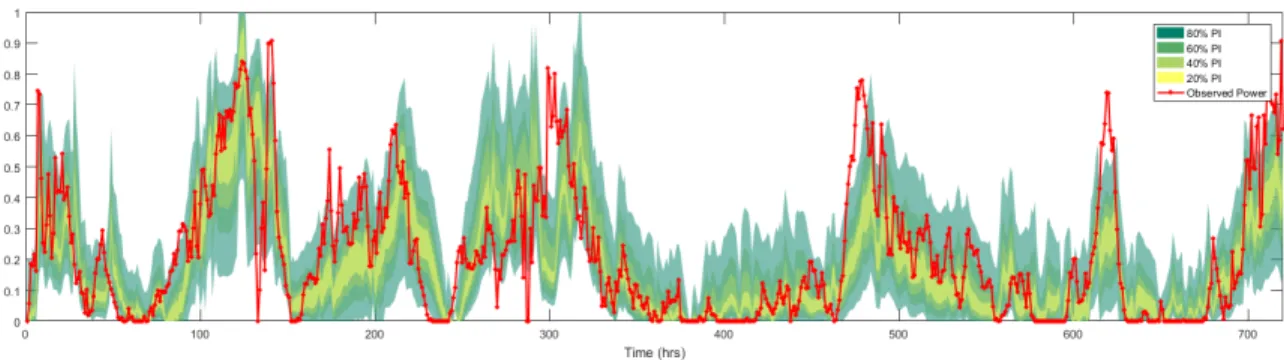
for U and V directions used as inputs to forecast wind power. (b) Observed wind power corresponding to the same time stamps. . . 83 4.2 Example plot of estimated 80%, 60%, 40%, and 20% prediction

in-tervals along with observed wind power in red for the month of July 2013. . . 84 5.1 Schematic diagram of the smooth pinball neural network. . . 93 5.2 Pinball ball function versus the smooth pinball neural network with

smoothing parameter α= 0.2. . . 94 5.3 Flowchart of the steps taken when conducting a probabilistic forecast

(14)

5.4 Reliability of prediction intervals from Zone 1 measured by the fre-quency of observation falling with each interval. . . 102 5.5 Sharpness of prediction intervals for Zone 1 measured by the interval

mean size. . . 103 5.6 QVSS measured relative performance of SPNN2, SPNN1, and SVQR

to QR on Zone 1 dataset. . . 104 5.7 Reliability of prediction intervals from Zone 2 measured by the

fre-quency of observation falling with each interval. . . 105 5.8 Sharpness of prediction intervals for Zone 2 measured by the interval

mean size. . . 106 5.9 QVSS measured relative performance of SPNN2, SPNN1, and SVQR

to QR on Zone 1 dataset. . . 107 5.10 Box plot of quantile score evaluation across all datasets. . . 108 5.11 Box plot of average coverage error evaluation across all datasets. . . . 109 5.12 Box plot of interval score evaluation across all datasets. . . 110 5.13 Box plot of sharpness evaluation across all datasets. . . 111 5.14 Bar plot of SPNN2 and SPNN1 mean quantile score across all wind

data compared to the performance of the top teams in GEFCom2014 Wind Track. . . 112 6.1 Pinball ball function versus the smooth pinball neural network with

smoothing parameter α= 0.2. . . 131 6.2 Architecture of the quantile Fourier neural network. . . 132 6.3 Flowchart of proposed methodology using QFNN. . . 133

(15)

6.4 Forecast comparison of the median quantile for the Sunspots time series (red dots) by QFNN (shown in black), SVQR (shown in blue), SARIMA (shown in green), and ETS (shown in purple). SVQR fails to capture any meaningful pattern in its prediction. SRIMA captures a seasonal pattern that is out of phase with the sunspot test series, and ETS shots off in the test set with a positive trend. QFNN cap-tured a seasonal pattern that is a bit more in phase with the number of sunspots over the years and is also able to learn multiple seasons of sunspots thus providing the most accurate quantile forecast of all the methods. . . 134 6.5 Forecast comparison of the median quantile for the Apple Closing

Stock Price time series (red dots) by QFNN (shown in black), SVQR (shown in blue), SARIMA (shown in green), and ETS (shown in pur-ple). SVQR can learn the linear trend of the stock series but nothing else. ETS learns a non-existing seasonal pattern, and SARIMA does not seem to capture any meaningful pattern. While QFNN does not have the highest accuracy regarding the QS and IS metrics we can see in the plot that it learns a cyclic trend of the stock price which follows the test set better than any other method. . . 135 6.6 Forecast comparison of the median quantile for the Load Demand

time series (red dots) by QFNN (shown in black), SVQR (shown in blue), SARIMA (shown in green), and ETS (shown in purple). SVQR captures a poor and small seasonal pattern. SRIMA captures the seasonality but fails to capture any cycles in the test set, and ETS shots off in the test set with a positive trend. QFNN learns both the seasonal and cyclical pattern of the load demand. . . 136

(16)

6.7 Forecast comparison of the median quantile for the Solar Power time series (red dots) by QFNN (shown in black), SVQR (shown in blue), SARIMA (shown in green), and ETS (shown in purple). SVQR is barely able to estimate the seasonality. SRIMA has a seasonal pat-tern reducing overtime in the test set, and while ETS captures the seasonality we see a negative trend. QFNN learns a constant seasonal quantile pattern that can be attributed to sunny days. . . 136 6.8 Forecast comparison of the median quantile for the Air Passengers

time series (red dots) by QFNN (shown in black), SVQR (shown in blue), SARIMA (shown in green), and ETS (shown in purple). SVQR estimates the trend but not the seasonality so well. ETS and SARIMA estimate both trend and seasonality well, but the median forecasts fall below and above the test data. QFNN learns the shape of the data better and appropriately captures the median. . . 137 6.9 Probabilistic forecasting of 50 prediction intervals for the Air

Passen-gers series. . . 137 6.10 Probabilistic forecasting of 50 prediction intervals for the Internet

Traffic series. . . 138 6.11 Probabilistic forecasting of 50 prediction intervals for the Load

De-mand series. . . 138 6.12 Probabilistic forecasting of 50 prediction intervals for the Solar Power

series. . . 139 6.13 Probabilistic forecasting of 50 prediction intervals for the Apple

Clos-ing Stock Prices time series. . . 139 6.14 Probabilistic forecasting of 50 prediction intervals for the Sunspots

time series. . . 140 6.15 Probabilistic forecasting of 50 prediction intervals for the simulated

Ocean Wave Elevation time series. . . 140 6.16 Probabilistic forecasting of 50 prediction intervals for the wind power

(17)

7.1 Example multi-step forecast from proposed QARNET model for load demand. Anomalous data is flagged when above or below the predic-tion intervals with a certain nominal coverage rate. . . 147 7.2 Example architecture of a convolutional neural network for regression. 148

(18)

Abstract

The presented research investigates the use of neural networks for probabilistic fore-casting in selected application areas. The topic of neural networks, also known as deep learning, has exploded as a research field, showing incredible results in image analysis and classification. But the application of neural networks to time series or regression-based forecasting is lesser known. Forecasting is the backbone of many industries and academic research areas. From predicting weather patterns to the stock market, to healthcare and energy, forecasting is vital to many operations of todays modern society. In the of evolution of the study of forecasting, the field of probabilistic forecasting has recently emerged. Unlike a deterministic forecast which only provides a single expected value, a probabilistic forecast provides information on the uncertainty of a prediction. We investigate how neural networks, which can automatically extract features via hidden layers, can be used to generate reliable and sharp probabilistic forecasts in the form of quantiles, prediction intervals, and full predictive densities. More specifically, we look at nonparametric probabilistic forecasting where we do not assume the underlying distribution of the forecasts. Our work seeks to evaluate these new methods in the application domains of renewable energies. In chapter 1 we provide a brief overview of probabilistic forecasting theory. In our first study (chapter 2) of this thesis, we overview the basic theory of how neural networks can be used for deterministic forecasting. This presents as a foun-dation for our later work for probabilistic prediction. In this study, we propose the development of an adaptive particle swarm optimization (APSO) learning algorithm to train a non-linear autoregressive (NAR) neural network, which we call PSONAR, for short term time series prediction of ocean wave elevations. We also introduce

(19)

a new stochastic inertial weight to the APSO learning algorithm. Our work is mo-tivated by the expected need for such predictions by wave energy farms. As such, we simulated noisy ocean wave heights for training and testing. We utilized our PSONAR to get results for 5, 10, 30, and 60-second multi-step predictions. Results show APSO can outperform backpropagation in training a NAR neural network.

In our second study (chapter 3) we study cyber-enabled demand-side manage-ment systems. DSM is a vital tool that can be used to ensure power system reliability and stability. In future smart grids, certain portions of a customers load usage could be under automatic control with a cyber-enabled DSM program which selectively schedules loads as a function of electricity prices to improve power balance and grid stability. In such a future, security of DSM cyberinfrastructure will be critical as advanced metering infrastructure, and communication systems are susceptible to hacking, cyber attacks. Such attacks, in the form of data injection, can manipulate customer load profiles and cause metering chaos and energy losses in the grid. These attacks are also exacerbated by the feedback mechanism between load management on the consumer side and dynamic price schemes by independent system operators. This work provides a novel methodology for modeling and simulating the nonlinear relationship between load management and real-time pricing. We then investigate the behavior of such a feedback loop under intentional cyber attacks using our feed-back model. We simulate and examine load-price data under different levels of DSM participation with three types of additive attacks: ramp, sudden, and point attacks. We applied change point and supervised learning methods for the detection of DSM attacks.

Results conclude that higher amounts of DSM participation can exacerbate at-tacks but also lead to better detection of such atat-tacks, point atat-tacks are the hardest to detect, and supervised learning methods produce results on par or better than sequential detectors. This chapter serves as an example of how linear methods can often yield better results then nonlinear such as neural networks. The need for deep learning or advanced probabilistic forecasting is not warranted in this DSM domain when generation is constant. However, we hypothesize that when renewable energy

(20)

more difficult. Due to the chaotic nature of renewable energies, there is a need to quantify the uncertainty in forecasting their power generation. As motivation and a prerequisite for future work to study DSM systems under renewable generation, in the next chapters we propose several new and advanced forecasting methods.

In our third study (chapter 4), we propose our first method to produce full pre-dictive densities by examining how support vector machines (SVMs) can be used for quantile estimation. SVMs are one of the most efficient machine learning al-gorithms, which is mostly used for pattern recognition since its introduction in the 1990s. Uncertainty analysis in the form of probabilistic forecasting can pro-vide significant improvements in decision-making processes in the smart power grid for better integrating renewable energies, particularly wind. This chapter analyzes the effectiveness of an approach for nonparametric probabilistic forecasting of wind power that combines support vector machines and nonlinear quantile regression with non-crossing constraints. A numerical case study is conducted using publicly available wind data from the Global Energy Forecasting Competition 2014. Mul-tiple quantiles are estimated to form 20%, 40%, 60% and 80% prediction intervals which are evaluated using the pinball loss function and reliability measures. Three benchmark models are used for comparison where results demonstrate the proposed approach leads to significantly better performance while preventing the problem of overlapping quantile estimates.

In our fourth study (chapter 5) we analyze the effectiveness of a novel approach for nonparametric probabilistic forecasting of wind power that combines a smooth approximation of a pinball loss function with a deep neural network architecture and a smooth penalty scheme to prevent the quantile crossover problem. We call our model the smooth pinball neural network (SPNN). A numerical case study is conducted using publicly available wind data from the Global Energy Forecasting Competition 2014. Multiple quantiles are estimated to form 10%, to 90% predic-tion intervals which are evaluated using a quantile score and reliability measures. Benchmark models such as the persistence and climatology distributions, multiple quantile regression, and support vector quantile regression are used for comparison where results demonstrate the proposed approach leads to improved performance

(21)

while preventing the problem of overlapping quantile estimates.

In our fifth study (chapter 6) we radically extend SPNN to forecast time se-ries. Point forecasting of univariate time series is a challenging problem with exten-sive work having been conducted. However, nonparametric probabilistic forecasting of time series, such as in the form of quantiles or prediction intervals is an even more challenging problem. To expand the possible forecasting paradigms we devise and explore an extrapolation-based approach that has not been applied before for probabilistic forecasting. We present a novel quantile Fourier neural network is for nonparametric probabilistic forecasting of univariate time series. Multi-step predic-tions are provided in the form of composite quantiles using time as the only input to the model. This effectively is a form of extrapolation based nonlinear quantile regression applied for forecasting. Experiments are conducted on eight real-world datasets that demonstrate a variety of periodic and aperiodic patterns. Nine simple and advanced methods are used as benchmarks including quantile regression neural network, support vector quantile regression, SARIMA, and exponential smoothing. The obtained empirical results validate the effectiveness of the proposed method of providing high quality and accurate probabilistic predictions. We then provide conclusions in our final chapter (chapter 7) as well as specific direction for future work.

(22)

Chapter 1

Introduction

In the last decade there have been two rising fields that have shown a lot of promise, unique results, and immense academic and industry attention. These are deep learning [1] and probabilistic forecasting [2]. Part of the success of deep learning, also known as the study of neural networks, is due to its ability to conduct automatic feature extraction at different levels of abstraction. Such feature extraction promotes by passes the need to provide manual feature engineering that is common among machine learning pipelines. Moreover, neural networks allow the representation of the nonlinearities in data, often associated with complex and real-world problems. Deep learning models have been used to achieve state-of-the art results in the field of computer vision [3] and have also been applied to the problem of forecasting [4]. However, the study of neural networks, and related methods, is limited when it comes to probabilistic forecasting. Thus, motivation for the presented research is to explore how neural networks could contribute to providing better probabilistic forecasts. Further motivation is provided by the new class of big data in regression and time series, which are vital in areas such as in the smart grid and renewable energy which are both used as application domains for our proposed forecasting frameworks.

(23)

Neural Networks

The study of neural networks has grown tremendously in the past decade. Neural networks are a set of algorithms, modeled very loosely after the human brain, that are designed to recognize patterns. They take in input data, which may come in different forms such as text, images, or time series, and they output either a class label for classification or a numeric value for regression. The layers of a network are made of computational nodes, again loosely modeled on a neuron in the human brain. These nodes take in data and perform some computation utilizing coefficients or weights which assign significance to inputs with regard to the task the algorithm is trying to learn. The weights can increase or decrease the significance of each data point. The input-weight products are fed into the node’s activation function, usually some nonlinear function, which then determines to what extent that signal should progress further through the network. Through utilizing a finite amount of nodes a neural network can approximate any continuous function, this is also known as the universal approximation theorem.

There are many types of neural networks including feedfward networks, recurrent networks, convolutional networks, deep belief networks and autoencoders. Due to the popularity of neural networks in both academic research and industrial applica-tion, there is already a large body of work reviewing the algorithms, mathematics, methods, approaches and issues. We therefore refer to the following references on the background of deep learning [1, 5–7], and in the next section we review in depth the field of probabilistic forecasting which has less literature.

Probabilistic Forecasting

Over the last several years there has been a large body of work conducted in nonparametric probabilistic forecasting. Recently the Global Energy Forecasting Competition in 2014 [8] and in 2017 [9] are further proof of the rising interest in probabilistic forecasting. Probabilistic forecasting is especially of large interest

(24)

to applications in renewable power such as wind. As such, the domain of wind forecasting is also part of the main focus of this dissertation. Wind forecasting models are either meteorological ensembles that are obtained by a weather model [10] or are statistical methods [11]. Under the statistical approach, we can estimate full predictive distributions in the form of quantiles or prediction intervals (PIs).

Some recent forecasting methods include extreme learning machines [13] where a direct quantile regression approach was presented to efficiently generate nonparamet-ric probabilistic forecasting of wind power generation combining extreme learning machine and quantile regression. Hybrid intelligent methods have also been ex-plored in [14] by feeding deterministic wind power forecasts made by a combination of wavelet transform and fuzzy ARTMAP network, optimized by using firefly opti-mization algorithm, in quantile regression. A PI estimation scheme is shown in [12] which uses a radial basis function neural network.Another approach to forecast the density of wind power is to take an ensemble of point forecasts and calculate the mean and variance of the combined forecasts. This has been studied in [15] where a wavelet transform and a convolutional neural network are used for ensemble point forecasting. Another ensemble approach can be seen in [16] where time series mod-els such as ARMA and GARCH are combined to form density forecasts. One of the most prevalent approaches to probabilistic forecasting of wind power is to ap-ply quantile regression (QR) which can be used to estimate different wind power quantiles [17].

Another alternative to nonparametric probabilistic wind forecasting is the ap-plication of the Lower Upper Bound Estimation (LUBE) method [18]. The LUBE method constructs a neural network with two outputs for estimating the prediction interval bounds. The coverage width-based criterion is used as the loss function for estimating PIs, and simulated annealing or particle swarm optimization [19] can be used to minimize that loss function. A complete review on probabilistic forecast-ing of wind power can be found in [17]. Other reviews on probabilistic forecastforecast-ing methods can be found in [20] for solar power, [8] for load forecasting, and [21] for electricity price forecasting.

(25)

forecasting, overview linear quantile regression, and summarize the main evaluation metrics for density forecasts. Given a random variableYtsuch as wind power at time t, its probability density function is defined asftand its the cumulative distribution

function asFt. IfFtis strictly increasing, the quantileq

(τ)

t of the random variableYt

with nominal proportionτ is uniquely defined on the value xsuch thatP(Yt < x) = τ. It can also be defined as the inverse of the distribution function q(_tτ) = F_t−1(τ). A quantile forecast ˆq(_t₊τ)_z is an estimate of the true quantile q(_t₊τ)_z for the lead time

t+z, given a predictor values (such as numerical wind speed forecasts). Prediction intervals are another type of probabilistic forecast and give a range of possible values within which an observed value is expected to lie with a certain probabilityβ ∈[0,1]. A prediction interval ˆI_t(₊β)_z is defined by its lower and upper bounds, which are the quantile forecasts ˆI_t(₊β)_z =hqˆ(τl)

t+z,qˆ

(τu)

t+z

i

=hl(_tβ), u_t(β)iwhose nominal proportionsτland τu are such that τu−τl = 1−β.

In probabilistic forecasting, we are trying to predict one of two classes of density functions, either parametric or nonparametric. When the future density function is assumed to take a certain distribution, such as the Normal distribution, then this is called parametric probabilistic forecasting. For a nonlinear and bounded process such as wind generation, probability distributions of future wind power, for instance, may be skewed and heavy-tailed distributed [22]. Else if no assumption is made about the shape of the distribution, a nonparametric probabilistic forecast

ˆ

ft+z [23] can be made of the density function by gathering a set of M quantiles

forecasts such that ˆft+z =

n ˆ q(τm) t+z , m= 1, ..., M|0≤τ1 < ... < τM ≤1 o with chosen nominal proportions spread on the unit interval. As mentioned before, renewable power forecasting can be quite stochastic, thus making nonparametric forecasting more ideal then fitting a parametric density [17].

1.0.1

Quantile Regression

Quantile regression is a popular approach for nonparametric probabilistic forecast-ing. Koenker and Bassett [24] introduce it for estimating conditional quantiles and is closely related to models for the conditional median [25]. Minimizing the mean

(26)

absolute function leads to an estimate of the conditional median of a prediction. By applying asymmetric weights to errors through a tilted transformation of the absolute value function, we can compute the conditional quantiles of a predictive distribution. The selected transformation function is the pinball loss function as defined by

ρτ(u) =

(

τ u if u≥0

(τ−1)u if u <0 , (1.1)

where 0 < τ < 1 is the tilting parameter. To better understand the pinball loss, we look at an example for estimating a single quantile. If an estimate falls above a reported quantile, such as the 0.05-quantile, the loss is its distance from the estimate multiplied by its probability of 0.05. Otherwise, the loss is its distance from the realization multiplied by one minus its probability (0.95 in the case of the 0.05-quantile). The pinball loss function penalizes low-probability quantiles more for overestimation than for underestimation and vice versa in the case of high-probability quantiles. Given a vector of predictorsXtwheret = 1, ..., N, a vector of

weightsW and intercept b coefficient in a linear regression fashion, the conditional

τ quantile ˆqτ is given by ˆq

(τ)

t =W>Xt+b. To determine estimates for the weights

and intercept we solve the following minimization problem

min W,b 1 N N X t=1 ρτ(yt−qˆ (τ) t ), (1.2)

whereytis the observed value of the predictand. The formulation above in Eq. (1.2)

can be minimized by a linear program.

There are many variations of QR which are traditionally solved using linear pro-gramming algorithms. In [26] local QR is applied to estimate different quantiles, while in [27] a spline-based QR is used to estimate quantiles of wind power. In [28] quantile loss gradient boosted machines are used to estimate many quantiles and in [29] multiple quantile regression is used to predict a full distribution with opti-mization achieved by using the alternating direction method of multipliers. Quantile regression forests [30] are another approach in forecasting which are an extension of regression forests based on classification and regression trees.

(27)

Due to their flexibility in modeling elaborate nonlinear data sets, artificial neural networks are another dominant class of machine learning algorithms that can be used to enhance QR. Taylor [31] is the first to propose a quantile regression neural network (QRNN) method, combining the advantages of both QR and a neural network. This method can reveal the conditional distribution of the response variable and can also model the nonlinearity of different systems. The author applies this method to estimate the conditional distribution of multi-period returns in financial systems, which avoids the need to specify the explanatory variables explicitly. However, the paper does not address how the network was optimized. The same QRNN was later used by [32] for credit portfolio data analysis where results showed that QRNN is more robust in fitting outliers compared to both local linear regression and spline regression. In [33] an autoregressive version of QRNN is used for applications to evaluating value at risk, and [34] implements the QRNN model in R as a statistical package.

1.0.2

Evaluation Metrics

In probabilistic forecasting it is essential to evaluate the quantile estimates and if desired also evaluate derived predictive intervals. Therefore, we reviews several im-portant evaluation metrics here. To evaluate quantile estimates, one can use the pinball function directly as an assessment called the quantile score (QS). We choose QS as our main evaluation measure for most of our studies for the following reasons. When averaged across many quantiles it can evaluate full predictive densities; it is found to be a proper scoring rule [35]; it is related to the continuous rank probability score; and it is also the main evaluation criteria in the 2014 Global Energy Forecast-ing Competition (GEFCOM 2014), the source of our testForecast-ing data. QS calculated overall N test observations and M quantiles is defined as

QS = N X t=1 M X m=1 ρτm(yt−qˆ (τm) t )

(28)

ob-quantiles for all look ahead time steps using equal weights. A lower QS indicates a better forecast.

With the QS calculated we can then also see what the relative performance of a proposed method is with respect to some benchmark method. We can assess relative performance between methods using the quantile verification skill score (QVSS) [36]

QV SS = 1− QS

f or QSref

where QSf or is QS for the forecast method of interest, and QSref is the QS value for the reference forecast of a benchmark method, which we will assume to be linear quantile regression. If QVSS is positive then forecast of interest performs better than the reference forecast, and a QVSS = 1 means a perfect forecast. Negative QVSS values indicate that forecast of interest performs worse than the reference forecast.

In some applications, it may be needed to have wind forecasts in the form of pre-diction intervals (PIs) and as such, we look at two secondary evaluation measures: reliability and sharpness. Reliability is a measure which states that over an evalua-tion set the observed and nominal probabilities should be as close as possible, and the empirical coverage should ideally equal the preassigned probability. Sharpness is a measure of the width of prediction intervals, defined as the difference between the upper uβi

t and lowerl βi

t interval values. For interval reliability we use the average

coverage error (ACE) metric [17] and for measuring interval sharpness we use the interval score (IS) which can also be used to evaluate the overall skill of PIs [37]. For measuring reliability, PIs show where future wind power observations are expected to lie, with an assigned probability termed as the PI nominal confidence (PINC) 100(1−βi)%. Here i = 1...M/2 indicates a specific coverage level. The coverage

probability of estimated PIs is expected to eventually reach a nominal level of con-fidence over the test data. A measure of reliability which shows target coverage of the PIs is the PI coverage probability (PICP), which is defined by

P ICPi = 1 N N X t=1 1{yt ∈Itβi(xt)}.

(29)

For reliable PIs, the examined PICP should be close to its corresponding PINC. A related and easier to visualize assessment index is the average coverage error (ACE), which is defined by

ACE =

M/2

X

i=1

|P ICPi−100(1−βi)|.

This assumes calculation across all test data and coverage levels. To ensure PIs have high reliability, the ACE should be as close to zero as possible. A high reliability can be easily achieved by increasing or decreasing the distance between lower and upper interval bounds. Thus, the width of a PI can also influence its quality. For measuring the effective width of PIs we use the sharpness score proposed by [23] which measures how wide PIs are by focusing on the mean size of the intervals only. We define ˆqu

t −qˆlt as the size of the central interval forecast with nominal coverage

rate (1−β). For lead times t = 1...Ntest, a measure of sharpness for PIs is then

given by the mean size of the intervals

Sharpness= 1 Ntest Ntest X t=1 (ˆq_tu−qˆl_t).

A lower sharpness score is considered more ideal, but too small and the PIs would not cover enough of the observed data. Thus sharpness is typically a measure to be considered along with reliability and a skill score. QS is a score that measures the skill of individual quantiles; to measure the skill of individual PIs we apply the interval score (IS) [37]. The IS - when evaluated with all test data and coverage levels - is defined by IS = 2 N M N X t=1 M/2 X i=1 (uβi t −l βi t )+ 2 βi (lβi t −yt)1{yt < ltβi}+ 2 βi (yt−uβti)1{yt> uβti} .

The prediction model is rewarded for narrow PIs and is penalized if the observation misses the interval. The size of the penalty depends on βi. Including all aspects

(30)

interval forecasts. However, IS cannot identify the contributions of reliability and sharpness to the overall skill. Thus, ACE and sharpness are both used for evaluation of PIs along with QS for evaluation of quantile estimation.

Outline of the Dissertation

The rest of this dissertation is organized as follows. Chapter 2 showcases our work in a recurrent neural network trained by particle swarm optimization for multi-step deterministic forecasting. This work highlights the background theory of deep networks for prediction and provides a base for building probabilistic forecasting neural networks in later chapters. In chapter 3 we present our work on modeling and detecting cyber demand side management attacks. This problem domain shows how nonlinear methods are not always better than linear ones. However, we propose that the incorporation of renewable generation such as wind, solar, and wave energy can complicate the attack problem. Thus, we are motivated to provide solutions that can forecast renewables and other nonstationary time series. In chapter 4 we propose a shallow neural network called constrained support vector quantile regression method for providing probabilistic forecasts of wind power. Next, in chapter 5, we expand to deeper neural networks trained by stochastic gradient descent and introduce a novel loss function and architecture for composite quantile estimation. In chapter 6, we extend our neural network models from ideas in signal processing and propose a novel multiple quantile Fourier neural network that applies to probabilistic forecasting of nonstationary univariate time series data. We evaluate this model on multiple domains. Finally, Chapter 8 concludes the dissertation, and we provide a number of extensions for future work in quantile neural networks. Fig. 1.1 outlines the reading order for this dissertation. Chapter 3 in detecting cyber-DSM attacks, deterministic forecasting methods are used. As such, chapters 1 and 2 should be read first. Chapters 4 to 7 describe neural network methods for probabilistic forecasting which should be read in that order. But before reading these chapters, chapters 1 and 2 should be read first which lay the foundations for neural network based prediction.

(31)

(32)

Chapter 2

Time Delayed Recurrent Neural

Network for Multi-Step Prediction

Introduction

Time-series prediction is an active area of research and an important practical problem in a variety of disciplines such as in energy forecasting, economics, finance, signal processing, and many other fields [38]. In the last two decades, artificial neural networks (ANNs) have been extensively applied for complex time series pro-cessing tasks [39]. This is due to their strength in handling nonlinear functional dependencies between past time series values and the estimate of the value to be forecasted.

Our main motivating factor in developing an accurate non-linear time series prediction method is for use in short term forecasting of renewable energy sources (RES). Such predictions are vital for integrating RES into existing power grids. Because of the variability in the generation of power from renewables gaps are left in the supply which must be filled by dispatchable resources and this is where prediction plays a key role. This is especially true in the new and active research area of controlling ocean wave farms and individual wave energy converters (WECs). In a wave farm sensors are located near WECs to measure ocean waveforms and relay

(33)

the information to the WECs, resulting in enhanced control and better interactions with the grid and markets.

In this work, we focus on using an ANN for the prediction of future wave el-evations at the measurement location. While waves are considered to be more predictable than other renewable energy sources such as wind or solar, the inter-mittency of wave energy is a big challenge in employing this resource as a reliable source of electric power in a generation portfolio. A demanding problem is the pre-diction of future levels of wave heights for operational scheduling and control in wave energy farms. The presented work is motivated by the fact that these predictions could allow new control methods to increase the efficiency of wave energy converter devices [40–42].

We have previously studied the use of a non-linear autoregressive (NAR) neural network trained using backpropagation which we called NARNET [43], to conduct multistep forecasts of wave power directly from observed wave heights. Long term predictions were made for several look ahead hours such as 3h, 6h, 12h, and 24h. The data used was significant wave height (SWH) which is the mean wave height of the highest third of the observed waves. This presents a challenge in testing accuracy of very short term predictions on the order of seconds. So in our current study we focus on shorter range forecasts which are obtained from simulated ocean wave height data rather than observed SWH data.

In this study we develop, test, and discuss a new method for nonlinear time series prediction. In enhancing the accuracy of our previous NARNET model while also using less memory in the training period, we used particle swarm optimization (PSO) for learning. We call this new model of using PSO to train a NAR neural network PSONAR. Since it is parametric it has all the advantages concerning estimation and testing connected with similar parametric methods. In addition, our neural network fulfills the requirements for the universal approximation theorem of neural networks [44] so it should be able to approximate any unknown nonlinear process. Further contribution comes in the form of our new stochastic inertia weight, a parameter used in our PSO learning algorithm, that emphasizes exploration more than exploitation

(34)

Background

A variety of different prediction approaches have been applied to forecast signals vital to reliably integrating RES into the power grid. Such diverse domains include weather, wave characteristics, wind speed, and electric load. Looking specifically at ocean waves, it has been traditional to apply physical models to predict wave heights [45] but there is a recent effort to utilize machine learning algorithms to train on past time series data to predict future forms. Various learning methods being tested range from regression to neural network models. Prediction of wave elevation levels has been done before for real time control of wave energy converters where the wave elevation is treated as a univariate time series and it is predicted only on the basis of its past history [46].

Predictive time series models like the auto-regressive (AR), auto-regressive mov-ing average (ARMA), and auto-regressive integrated movmov-ing average (ARIMA) have been found suitable for forecasting in a number of different domains. AR and ARMA models specifically are appropriate for stationary time series, while ARIMA and other models such as Kalman filters are aimed at non-stationary data and long-term series. These models therefore have also found widespread use in the simulation and estimation of the wave characteristics based on historical data [39]. Alternatively, artificial neural networks (ANN) have been found equally useful and even shown to outperform ARMA models [47]. Due to their high performance, we chose ANNs for prediction. In an ANN, forecasting is done by feeding a sequence of previous observations to the model as input so that it can recognize hidden patterns in the series and consequently estimate future values. Neural networks have been applied to study aspects of waves such as predicting the height of a wave at the time of its breaking and the depth of water at which it breaks [48].

An ANN can be trained by any number of learning algorithms, the most well known one being gradient descent backpropagation. Another lesser known alterna-tive is particle swarm optimization (PSO). In 1995, Dr. Eberhart and Dr. Kennedy

(35)

developed PSO which is a population based stochastic optimization strategy, in-spired by the social behavior of a flock of birds [49]. PSO is similar to Genetic Algorithms (GA) in terms of population initialization with random solutions and searching for global optima in successive generations [50]. But unlike GA, PSO does not undergo crossover and mutation, instead the particles move through the problem space following the current optimum particles. When using PSO, a possible solution to an underlying numeric optimization problem is represented by the position of a particle in the search space. PSO is suggested to be a powerful training algorithm for ANNs [51–54].

PSO is a powerful global optimization algorithm which has been successfully hybridized with genetic algorithms [55], fuzzy logic [56], and support vector machines [57] for application in various domains. In related work, using PSO to train ANNs for prediction has also been used in the past such as [58–62]. However, most of these cases only looked at single time step prediction and did not consider predicting hundreds of future data points instantaneously. Some of these papers also did not consider the effect of training using an adaptive inertial weight in the PSO algorithm which could dynamically change the velocity of a particle. Our contributions look at these factors.

Neural Network Model

In predicting a time series which exhibits volatile behavior, a number of different ANNs have been found particularly useful [63]. A popular ANN model for time series prediction is the Nonlinear Auto Regressive model with eXogenous inputs (NARX) neural network [64]. This is a network with tapped time delay inputs and has recurrent dynamic feedback connections enclosing the layers. The output of the network is fed back into the input of the model. It is a combination of a multilayered perceptron, a simple recurrent network, a time delayed network, and a feedfoward backpropagation network. Fig. 2.1 shows a NARX network with the feedback element and one hidden layer. Below we first describe the structure of the

(36)

Figure 2.1: Example of a NARX network. NARX model y(n) = f(x(n−1), x(n−2), . . . , x(n−mx), . . . ,xˆ(n−1), ˆ x(n−2), . . .xˆ(n−mˆx))

where x(n) and ˆx(n) symbolize, respectively, the input and output functions of the neural network at time n, while mx and mˆx represent the input and output

memory order, and f is a nonlinear function. The function f is approximated by a multilayered perceptron. The output at time-step n is dependent on its past

mxˆ values and the past mx input values. The network uses a time-delayed (TDL)

architecture with a feedback connection from the output layer to the input layer of the network. States in the NARX network are updated as

(37)

xi(n+ 1) =        u(n) i=mx y(n) i=mx+my xi+1(n) 1≤i < mx OR mx < i < mx+my

so that at time n the tap delays correspond to the values

x(n) =

{u(n−mx), . . . , u(n−1), y(n−my), . . . , y(n−1)}

The MLP approximation of the function f consists of a set of nodes organized into two layers. There arei= 1...N inputs andh= 1...q nodes in the hidden layer. Each hidden node performs the following function

zh(n) =σ N X i=1 wihxi(n) +bh ! ,

whereσ is the nonlinear transfer function

σ = 1

1 +e−x

andwih∈WH are the weights between the input and output layer andbh ∈BH are

the weights of the bias term in the network, given by

WH =     wH₁_,₁ · · · w₁H_,i .. . . .. ... wH q,1 · · · wq,iH     , BH     bH₁ .. . bH q     .

The output layer consists of a single linear node

y(n) =

q

X

h=1

whzh(n) +θo,

(38)

WO =     wO₁ .. . wO q     .

An advantage of the NARX architecture is that it can converge faster and gen-eralize better than other networks [63]. In our experiments we specifically use a derivative of the NARX network known as the non-linear autoregressive (NAR) neural network where we do not have exogenous inputs. During testing, predicted values at each time step are the only inputs fed to the network. Diving deeper into the training and testing of our network, we differentiate between two modes of operation similarly based on the NARX network modes of operation from [65].

We call the first one series mode, shown in Fig. 2.2; this is used during training. Here the network has a purely feedforward architecture and a learning algorithm such as backpropagation can be used for training. The second one is called parallel mode in which the output is fed back to the input of the feedforward neural network as part of the standard NARX architecture, as shown in Fig. 2.3, with the DELAY being the tapped delay line. The series mode NAR network is converted to the parallel mode to perform the prediction during testing. Our NAR network has an input layer of neurons, an output layer, and one hidden layer. We previously used the Lavenberg-Marquardt backpropagation algorithm as a training function to update the weight and bias values of the NAR model [43], we call this neural network NARNET.

Particle Swarm Optimization

PSO is a stochastic global optimization algorithm which is based on the sim-ulation of the social behavior of a swarm. It exploits a popsim-ulation of candidate solutions in a search space. The particles in the swarm are initialized with a pop-ulation of random solutions which will move through the N-dimensional problem space to search for new potential solutions. A fitness, f, is then calculated as a

(39)

Figure 2.2: NAR network series mode.

Figure 2.3: NAX network parallel mode.

certain measure of quality in reaching a target value. Each particle i is associated with two vectors, the velocity vector Vi = [vi1, vi2, ..., xNi ] and the position vector

Xi = [x1i, x2i, ..., xNi ] and are updated as follows

− →_v i(t+ 1) = − →_v i(t) +c1φ1(→−pi(t)− −→xi(t)) +c2φ2(−→pg(t)− −→xi(t)) − →_x i(t+ 1) =−→xi(t) + ∆t−→vi(t+ 1).

(40)

The first equation updates a particle’s velocity which is a vector value with multiple components. The term−→vi(t+ 1) is the new velocity at timet+ 1. The new velocity

depends on three terms. The first term is−→v i(t), the current velocity at time t. The

second part is c1φ1(−→pi(t)− −→xi(t)). The c1 term is a positive constant called the

coefficient of the self-recognition component. The φ1 and φ2 factors are uniformly

distributed random numbers in [0,1]. The −→pi(t) vector value is the particle’s best

position found so far. The −→xi(t) vector value is the particle’s current position. The

third term in the velocity update equation is c2φ2(−→pg(t)− −→xi(t)). Thec2 factor is

a constant called the coefficient of the social component. The −→pg(t) vector value is

the best known position found by any particle in the swarm so far. Once the new velocity, −→v i(t+ 1), has been determined, it is used to compute the new particle

position −→xi(t + 1). The term −→v i is limited to the range ±−→vmax. ∆t is a time

delay in updating a particles position, which is usually set to 1. The personal best position of a particle is calculated as:

− →_p i(t+ 1) = ( −→ pi(t) if f(−→xi(t+ 1))≥f(−→pi(t)) − →_x i(t+ 1) if f(−→xi(t+ 1))< f(−→pi(t)),

wheref is the fitness function. PSO does not require a large number of parameters to be initialized. But the choice of PSO parameters can have a large impact on optimization performance and has been the subject of much research [66]. For most practical applications, a typical choice of the number of particles is in the range from 10 to 40. Usually, 20 particles is sufficient to get good results. In the case of more difficult problems, the choice can be increased to 100 - 200 particles. Parametersc1

and c2, (the coefficients of self-recognition and social components respectively) are

not critical for the convergence of the PSO algorithm, but fine-tuning these learning vectors aids in faster convergence and alleviation of local minima. It is suggested to set these parameters to c1 =c2 = 2 [49]. An alternative could be to choose a larger

self-recognition component, c1, than the social component, c2, such that it satisfies

conditions such as c1+c2 = 4 [67].

The particle dimension and range is determined based on the problem to be optimized. Various ranges can be chosen for different dimension of particles. Usually

(41)

Figure 2.4: The scheme for value of the inertia weight w.

the range of particles is set as the maximum velocity. For instance, if a particle belongs to the numeric range -5 to 5, then the maximum velocity is 10. The stopping criteria may be any one of the following: the process can be terminated after a fixed number of training epochs or iterations such as 1000, or the process may be terminated when the error between the obtained objective function value and the best fitness value is less than a specified threshold.

2.0.1

Adaptive PSO

The adaptive particle swarm optimization (APSO) algorithm is based on the original PSO algorithm and is described below:

− →_v

i(t+ 1) =

(42)

Theω factor is called the inertia weight. The inertia weight plays an important role in the convergence behavior of the PSO algorithm. The inertia weight is employed to control the impact of the previous history of velocities on the current one. Ac-cordingly, the parameter ω regulates the trade-off between the global exploration and local exploitation abilities of the swarm. A large inertia weight aids in global exploration (searching wide ranging areas), while a small inertia weight aids in local exploitation (searching within the nearby areas). To obtain a balance between the global and local searches the number of iterations required to locate the optimum solution are reduced. The inertia weight is usually set as a constant initially and in order to promote global exploration of the search space, the parameter is gradually decreased to get more optimal solutions.

There are several variants of using an inertia weight. The inertia weight proposed by Shi and Eberhart [68] decreases with iterative generations as:

ω=ωmax−(ωmax−ωmin) g G

where g is the current iteration index, G is the predefined maximum number of training epochs, and ωmax and ωmin are the maximal and minimal weights. From

empirical experimentation we have devised a slight variation of the inertia weight which we call a stochastic initial weight:

ω=ωmin+φ(ωmax−ωmin) g G

whereφ is a normally distributed random number at each iteration. Our measure is contradictory to the idea of having the inertia weight decrease over time. However, we believe the increased exploration allows the particles to search more broadly over time for new solutions in order to minimize the fitness function. Fig. 2.4 shows the change inω over iteration where it increases stochastically over time.

PSO for Training of Neural Networks

In the case of training a neural network through PSO, a particle’s position repre-sents the values for the network’s weights and biases. The goal is to find a position

(43)

so that the network generates computed outputs that match the outputs of the training data. PSO is initialized with a group of random particles. In one epoch or iteration, each particle is updated by following two best values. The first one is the best weight solution achieved so far by each individual particle’s best position. An-other best value tracked by the particle swarm optimizer, are the global best weight values, obtained by any particle in the population; so, the velocity and position of the obtained optimum solution is updated during an iterative process. The stop criteria are reaching the maximum iteration number or satisfaction of the minimum error condition.

Fig. 2.5 illustrates the flowchart of training a NAR neural network with PSO which we call our PSONAR network. The first step is initialization. The network is first constructed by choosing the number of input, hidden, and output node parameters. Then all the PSO variables such asc1, c2, dt, Vmax,etc, and termination

conditions are chosen. These parameters have a very important effect to promote the networks efficiency. The position vectors Xt and velocity vectors Vt are initialized

randomly between 0 and 1. Here the training data can also be preprocessed. In the training algorithm, the search space is N-dimensional where N is set by the total number of weights and biases in the network between the input and hidden layer, and the hidden and output layer. The position coordinates of each particle

xi(t) in the search space is then the following weights:

xi(t) = ( w1 ih, w2ih, ..., wnih, w1 ho, w2ho, ..., whom ) ,

where wIHn represents all the weights between the input and hidden nodes and wHOmrepresents all the weights between the hidden layered nodes and output node.

During training, weights and biases of the NAR network are set to the calculated positions of the given particle. Then all training data is fed into the network for a given particle’s weights to get the network’s outputs. We then use the mean squared error (MSE) as our fitness function. If the MSE is below a threshold then training ends. If not then the pBest score of the given particle’s best position pi(t)

(44)

(45)

Figure 2.6: 3D plot of spatial distribution of simulated ocean waves.

(46)

Figure 2.8: 10 second lookahead (20 steps) PSONAR prediction example.

is set to the MSE andpi(t) is set to the current positionxi(t). The global best of all

the particles is compared to the fitness MSE. If it is greater, then the gBest score is set to the MSE andPg(t) is set to the current positionxi(t). Next the position and

velocity vectors of the current particle are updated. If at this point the maximum number of epochs has been reached then training stops. Otherwise the next particle in the swarm is evaluated in the network. While we use one hidden layer in our PSONAR, the training algorithm can easily be scaled to include multiple hidden layers.

(47)

Experimental Setup

2.0.2

Data Source

For our analysis, we use the well accepted standard wave equation model from [69] where we assume the ocean is an ideal incompressible fluid with no loss of mechanical energy. We also adopt the common assumptions that the fluid motion is irrotational and that the wave amplitudes are small enough so that linear theory is applicable. Moreover, the deployment area in the ocean is assumed to be of sufficient depth such that finite depth effects, other than dispersion, are small. Finally, we assume that the waves were created by forcing functions, distant storms for example, that were applied at sufficient distances away resulting in the observation of fully developed ocean waves. Under the assumptions just described, the solutions for the simplified differential wave equation are plane waves consisting of a sum of sinusoids with different amplitudes, frequencies, directions, and phases. Therefore, we assume that wave elevations under a local wave field are described by plane waves having, in total, M directions and frequencies. Then, for all two dimensional sensor locations (x, y)T _{on the surface, all times} _t _{of interest, the exact phase-resolved}

(wave-by-wave) wave elevation η(x, y, t) which would be observed at a particular location in the deployment area is described by

η(x, y, t) = M X i=1 Aicos (w 2 i g )(xcos(βi) +ysin(βi))−twi+φi ,

whereAi is the amplitude in meters, ωi is the frequency in radians per second,βi is

the angular direction in radians measured relative to the x-axis, φi is the phase in

radians, andg is the acceleration due to gravity in m_s2.

Using the just described model for the wave elevation, we assumed a local wave field that is described by five component plane waves, each having its own amplitude, frequency, direction, and phase. The sets used to describe the wave field were A=

(48)

Figure 2.9: 10 second lookahead (20 steps) NARNET prediction example.

φ = {2,1,3,0.3,0} where Ai, wi, βi, φi are the amplitude, frequency, direction, and

phase of the ith component wave, where i = 1,2, . . . ,5. These values are chosen based on typical values reported in experiments and observations found in [69–71]. A snapshot of the assumed wave field is given in Fig. 2.6.

The training data is then taken to be the wave elevation measurements taken at the origin for 250 seconds, starting at time equal to zero, sampled at 2 Hz or one sample every half a second observed under independent additive white Gaussian noise with zero mean and 0.01 variance (minor noise) and second set with zero mean and 0.25 variance (some noise). A sample window of 30s of data with noise is shown in Fig. 2.7.

(49)

2.0.3

Error Measurements

Error measurement statistics play a critical role in analyzing forecast accuracy, ob-serving exceptions, and benchmarking methods. In our results we use five error statistics, so that we can prove a broad comparison metrics for future studies, and we provide confidence intervals for predicted values. We first use the mean absolute percentage error (MAPE) which measures the size of the error in percentage terms and is a common estimate of error in forecasting problems. MAPE is defined as

M AP E = 1 N N X i=1 xi−yi xi ,

where N, is the total number of predicted values, xi is the actual observed value,

and yi is the forecasted value by the neural network. We also calculate the mean

square error (MSE) and root mean squared error (RMSE) to evaluate accuracy

M SE = 1 N N X i=1 (xi −yi)2, RM SE = √ M SE.

We then use the mean absolute deviation (MAD) which measures the size of the error in units. MAD takes the absolute value of forecast errors and averages them over the entirety of the forecast time periods. It is calculated as the mean of the unsigned errors M AD= 1 N N X i=1 |xi−yi|.

Lastly we use the Pearson’s correlation coefficient (CC) which is a measure of the linear dependency between two variables, in our case the observed and forecasted values, and is calculated as

CC = PN i=1(xi−x)(yi−y) q PN i=1(xi−x) 2PN i=1(yi −y) 2 .

A confidence bound for a model or variable is an interval of values within which we expect the true value of the population parameter to be contained. For calculating

(50)

Figure 2.10: Convergence plot of PSONAR in Fig. 2.8.

bounds for our model we use the bootstrapping method [72] which resamples resid-uals for estimating the variance of forecasted values at each time step. The upper and lower endpoints are specified as

Y ±z√σ n,

withY representing the sample mean (center of the confidence interval),σ/√nbeing the standard deviation of the sampling distribution, andz is a constant multiplier set at 1.96 for a 95% confidence interval.

Results

The PSONAR neural network is used to predict results of up to 5, 10, 30, and 60 second forecasts where each forecast is composed of 10, 20, 60, and 120 prediction steps. The max number of training epochs was set to 1000. The NAR

(51)

network for both PSONAR and NARNET has 1 hidden layer and empirically we chose them to have 10 input nodes and 14 hidden node each. For the PSONAR network we chose the coefficient of self-recognition to have a weight of 2.5 and the social component to have a weight of 1.5. For the stochastic inertial weight we set ωmax = 0.9 and ωmin = 0.4. Fig. 2.10 shows an MSE convergence plot for an

example prediction using PSONAR whose results are showcased in Fig. 2.8. Fig. 2.9 shows the same sample experiment run with the NARNET. Error statistics of the plots are summarized in Table II.

Table 2.1: Table of error statistics with minor noisy data.

PSONAR 5s 10s 30s 60s MSE 0.1626 0.7284 6.3961 9.8831 RMSE 0.4033 0.8535 2.5290 3.1437 MAPE 0.3428 0.4302 1.5131 4.5228 MAD 0.3437 0.7399 2.0099 2.5102 CC 0.9972 0.9643 0.4944 0.0103 NARNET 5s 10s 30s 60s MSE 0.1531 1.3392 7.2867 11.4703 RMSE 0.3912 1.1572 2.6993 3.3867 MAPE 0.2033 0.7033 1.3948 3.4318 MAD 0.3161 0.8971 2.0568 2.6227 CC 0.9971 0.9332 0.4980 0.2076

Table I shows the error statistics for multistep prediction on data with minor additive white Gaussian noise. Table II shows the error statistics for data with more noise. As seen in the two tables, for 5s lookahead prediction the NARNET using gradient descent backpropagation for learning performed better. Looking further into the future PSONAR outperformed the NARNET network to a small extent.

(52)

Table 2.2: Table of error statistics with higher noisy data. PSONAR 5s 10s 30s 60s MSE 0.2097 0.9153 8.9066 13.4073 RMSE 0.4579 0.9567 2.9843 3.6615 MAPE 0.1734 0.2964 2.0758 3.2429 MAD 0.3470 0.6783 2.4161 2.8644 CC 0.9974 0.9693 0.3743 0.0902 NARNET 5s 10s 30s 60s MSE 0.1603 1.4119 10.8491 14.0818 RMSE 0.4003 1.1882 3.2937 3.7525 MAPE 0.2531 0.7421 1.3229 4.7647 MAD 0.3698 0.8938 2.0769 3.0842 CC 0.9971 0.9165 0.31433 0.12301

Conclusion

This work proposed a method for using particle swarm optimization to train a non-linear autoregressive neural network. The accuracy of our proposed PSONAR is tested using ocean wave heights for the purpose of aiding the integration of wave energy into the power grid. As such, we believe our scheme will be helpful in multi-step prediction as needed in integrating other stochastic renewable resources, such as wind or solar. Moreover, compared to existing methodologies, the PSONAR can be applied to other applications where predictions are needed for multiple time steps. Our method of using a stochastic inertial weight in the PSO learning algorithm to train our NAR neural network with simulated data showed successful results in predicting short term ocean wave levels. Results show PSO can outperform backpropagation.

In this study we ran experiments on one test set and used only a single set of parameters for initializing the neural networks and the PSO learning algorithm. Further work is planned to compare results of the stochastic inertia weight with a decreasing inertia weight, expand the number of testing sets, test the effect of varying the number of neural nodes and hidden layers, and provide a deeper computational

(53)

analysis such as usage of memory and error analysis. We plan to also test a number of PSO variants such as Clan PSO [58, 73], Trelea PSO [74], hybrid backpropagation PSO [51], and other swarm methods such as ant colony optimization [75]. We would then evaluate their effectiveness as training algorithms for training a NAR network for time series prediction by running a Monte Carlo method to obtain a distribution of multiple runs with each comparative method. In these studies we plan to incorporate both simulated data and actual data from buoy sensors for wave height elevations for studies in wave energy farm and wind speeds for studies in wind energy farms.

(54)

Chapter 3

Detection of Cyber-DSM Attacks

using Forecasting and Supervised

Learning

Introduction

In this chapter we examine a new domain of cyber enabled demand side manage-ment (DSM). We study this domain in depth, provide a mathematical framework for it, and showcase it’s vulnerabilities to attacks with the main goal to detect such attacks. We introduce this problem to determine if its structure requires the need of deep learning and forecasting. A number of statistical and machine learning meth-ods are used for the detection of attacks and we provide an analysis if linear or nonlinear methods in this ca