CU Scholar
Civil Engineering Graduate Theses & Dissertations
Civil Engineering
Spring 1-1-2012
Stochastic Weather Generator Based Ensemble
Streamflow Forecasting
Nina Marie Caraway
University of Colorado at Boulder
Follow this and additional works at:
http://scholar.colorado.edu/cven_gradetds
Part of the
Civil Engineering Commons
,
Environmental Engineering Commons
, and the
Hydrology Commons
This Thesis is brought to you for free and open access by Civil Engineering at CU Scholar. It has been accepted for inclusion in Civil Engineering
Graduate Theses & Dissertations by an authorized administrator of CU Scholar. For more information, please contact
[email protected]
.
Recommended Citation
Caraway, Nina Marie, "Stochastic Weather Generator Based Ensemble Streamflow Forecasting" (2012).
Civil Engineering Graduate
Stochastic Weather Generator Based Ensemble Streamflow
Forecasting
by
Nina Marie Caraway
B.E., Vanderbilt University, 2010
A thesis submitted to the
Faculty of the Graduate School of the
University of Colorado in partial fulfillment
of the requirements for the degree of
Master’s of Science
Department of Civil Engineering
2012
Stochastic Weather Generator Based Ensemble Streamflow Forecasting
written by Nina Marie Caraway
has been approved for the Department of Civil Engineering
Balaji Rajagopalan
Edith Zagona
Date
The final copy of this thesis has been examined by the signatories, and we find that both the
content and the form meet acceptable presentation standards of scholarly work in the above
iii
Caraway, Nina Marie (M.S., Civil Engineering)
Stochastic Weather Generator Based Ensemble Streamflow Forecasting
Thesis directed by Prof. Balaji Rajagopalan
On a seasonal time scale, forecast centers of National Weather Service produce streamflow
forecasts via a method called Ensemble Streamflow Prediction (ESP). In conjunction with the
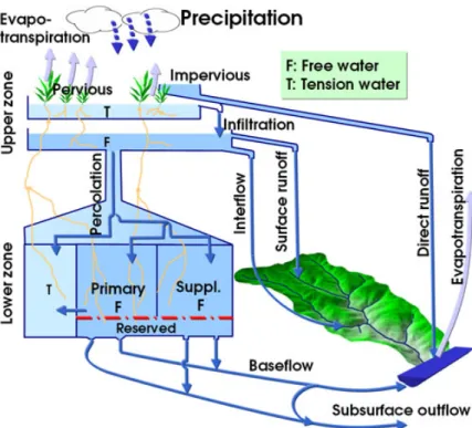
physically-based Sacramento Soil Moisture Accounting model (SAC-SMA), ESP uses historical
weather sequences for the forecasting period starting from model’s current initial conditions, to
produce ensemble streamflow. There are two major drawbacks of this method—(i) the ensembles are
limited to the length of historical record thereby producing limited variability and (ii) incorporating
seasonal climate forecasts such as El Ni˜
no Southern Oscillation (ENSO) is done by selecting a subset
of historical sequences which further reduces the variability of streamflow forecasts. The need for
alleviating these drawbacks motivates the proposed research. To this end, this research effort has
two components (i) an improved multi-site stochastic weather generator and (ii) coupling it to the
SAC-SMA model for ensemble streamflow forecasting.
We enhanced the traditional K-nearest neighbor semi-parametric stochastic weather
gener-ator (SWG). In SWG the daily precipitation state (wet or dry) is modeled as a Markov Chain
and the weather vector on a given day is simulated conditioned on the previous day’s precipitation
state and weather vector and current day’s precipitation state. A K-nearest neighbor resampling
approach is used to simulate from the conditional probability density function. Our improvements
to this stochastic generator include (i) clustering the locations into climatologically homogeneous
regions and applying the weather generator separately for each region and jointly to better capture
the spatial heterogeneity and, (ii) modifying the resampling approach to incorporate
probabilis-tic seasonal climate forecast. We tested this enhanced weather generator by applying it to daily
weather sequences at 66 locations in the San Juan River Basin. The proposed method generates a
rich variety of weather sequences capturing the distributional properties at all the locations and the
spatial dependence. It also simulates consistent weather sequences conditioned on seasonal climate
forecasts.
The multi-site stochastic weather generator was coupled with the SAC-SMA model
(WG-ESP) within NWS’s new Community Hydrologic Prediction System (CHPS) to produce ensemble
streamflow forecast. Spring season ensemble forecasts at several lead times from Nov through Apr
for the period 1981–2010 were made from WG-ESP and the traditional ESP for the San Juan River
Basin. We show that the weather generator based ensemble produces a rich variability in the flows
including extremes and a higher skill at long lead times. Especially, skill in wet year forecast was
found to be higher than dry years.
The flexible and robust framework provides many opportunities to further improve the ESP
system in enabling increased skills at longer lead times that will be of immense help to water
resources managers.
Dedication
Acknowledgements
Firstly I would like to thank my advisor Balaji for his guidance on this project and for
exposing me to the fascinating world of data analysis. I would like to thank my second member
Andy for all of his invaluable help in sending data, explaining NWS methodologies, and helping
the set-up and subsequent running of CHPS. Also, I would like to thank Edie for serving as the
third member of my committee and for hosting me and providing computational resources for me
at CADSWES.
A special thanks goes to Cameron for helping me develop my programming skills and for
dealing with my now painfully-dumb sounding coding questions. Jason gets a thanks for converting
the weather generator codes from FORTRAN to R. Thank you James for helping me set up an
account on your group’s NASA machine. Additionally, thanks for introducing me to a bevy of
R techniques, for all of your help developing cluster methods for the weather generator, and for
helping write the weather generator paper.
Thank you Lisa for being a great office mate and thanks to all in my research group for our
incredibly-helpful meetings (and happy hours).
Finally, I would like to thank Kevin and others at the CBRFC for their help and NOAA for
their funding of this project.
vii
Contents
Chapter
1
Introduction
1
1.1
Background . . . .
1
1.2
Study area and context . . . .
3
1.3
Thesis outline . . . .
4
2
Multisite Stochastic Weather Generation Using Cluster Analysis and K-nearest neighbor
Time Series Resampling
5
2.1
Introduction . . . .
5
2.2
Study Region, Application Context and Data . . . .
8
2.3
Methodology . . . 10
2.3.1
Cluster Analysis . . . 10
2.3.2
Spatial Precipitation Occurrence Model . . . 11
2.3.3
K-NN Resampling . . . 12
2.4
Results . . . 16
2.4.1
Clusters . . . 18
2.4.2
Unconditional Simulation . . . 21
2.4.3
Conditional Simulation . . . 36
3
Advancing Ensemble Streamflow Prediction with Stochastic Meteorological Forcings for
Hy-drologic Modeling
49
3.1
Introduction . . . 49
3.2
Proposed Framework . . . 52
3.2.1
Current Methodology . . . 52
3.2.2
Proposed Improvement
. . . 55
3.3
Application Region and Data . . . 56
3.3.1
Basin Characteristics . . . 56
3.3.2
Data . . . 57
3.4
Results . . . 59
3.4.1
Forecast Skill Evaluation . . . 61
3.4.2
Unconditional Forecasts . . . 64
3.4.3
Conditional Forecasts . . . 77
3.5
Summary and Discussion . . . 86
4
Conclusion
89
4.1
Summary and Conclusions . . . 89
4.2
Recommendations for Future Work . . . 90
Bibliography
92
Appendix
A
Additional CHPS Figures
98
A.1 Unconditional . . . 98
A.2 Conditional . . . 125
ix
Tables
Table
2.1
K
-nearest neighbors for ordinal day of December 9th: unconditional simulation . . . 15
2.2
Same as Table 2.1, but for wet simulation with ANB of 65:25:10 . . . 16
2.3
Number of stations falling within each cluster . . . 18
3.1
Characteristics of representative locations (gages) . . . 59
3.2
P-values from two-sided t-tests of April to July runoff . . . 76
3.3
P-values from Wilcoxon rank sum test for 2005 and 2006 April to July runoff . . . . 83
A.1 P-values from two-sided t-tests of April to May runoff . . . 123
A.2 P-values from two-sided t-tests of June to July runoff
. . . 124
A.3 P-values from Wilcoxon rank sum test for 2005 and 2006 April to May runoff . . . . 140
Figures
Figure
2.1
San Juan Watershed: the four corners of Utah, Colorado, New Mexico, and Arizona
is just above the center of the figure . . . .
9
2.2
Uncertainty in the within sum of squares (WSS) as a function of
k
th for 50
indepen-dent clusterings of total seasonal precipitation over 66 stations in 29 years. . . 17
2.3
DJF geographical clustering of observation locations by seasonal total precipitation . 19
2.4
Same as Figure 2.3 for JJA . . . 20
2.5
Histograms of between-cluster correlations in the observed data for all stations in
each pair of clusters . . . 22
2.6
Smoothed probability densities of basin-total seasonal precipitation for all methods . 23
2.7
Average number of wet day occurrences per season plotted against observed for each
approach . . . 24
2.8
Smoothed probability densities of cluster-total seasonal precipitation for all methods
25
2.9
Simulated and observed distributions of between-cluster correlations . . . 27
2.10 Root mean square error over all locations and simulations . . . 28
2.11 Simulated versus observed lag-1 autocorrelations . . . 29
2.12 Distribution (over all simulations) of differences between observed and simulated
statistics of precipitation . . . 31
2.13 Same as Figure 2.12 for max temperature . . . 32
2.14 Same as Figure 2.12 for min temperature . . . 33
xi
2.15 DJF cumulative probability density of temperature spells at three individual sites.
Spell thresholds corresponding to quantile are shown with the location name in the
individual titles. The median simulation at each site is shown. . . 34
2.16 Same as Figure 2.15 for JJA . . . 35
2.17 Cumulative probabilities of conditional, within-cluster seasonal precipitation totals
for DJF, with black being historical
. . . 38
2.18 Same as Figure 2.17 for MAM . . . 39
2.19 Same as Figure 2.17 for JJA . . . 40
2.20 Same as Figure 2.17 for SON . . . 41
2.21 Shifts in exceedance risk for conditional within-cluster DJF seasonal totals . . . 42
2.22 Same as Figure 2.21 for MAM . . . 43
2.23 Same as Figure 2.21 for JJA . . . 44
2.24 Same as Figure 2.21 for SON . . . 45
3.1
Sacremento soil moisture accounting model schematic (Werner, 2011a) . . . 54
3.2
ESP flow chart . . . 54
3.3
ESP flow chart with weather generator input . . . 55
3.4
San Juan Watershed . . . 58
3.5
Historical April–July runoff volumes for representative locations with averages shown
by dotted lines . . . 60
3.6
BFFU1 ESP April to July reforecasts for November to April lead times . . . 65
3.7
DRGC2 ESP April to July reforecasts for November to April lead times . . . 66
3.8
April to July BFFU1 WG ESP vs ESP moments . . . 68
3.9
April to July DRGC2 WG ESP vs ESP moments . . . 69
3.10 April to July median and mean RPSS . . . 70
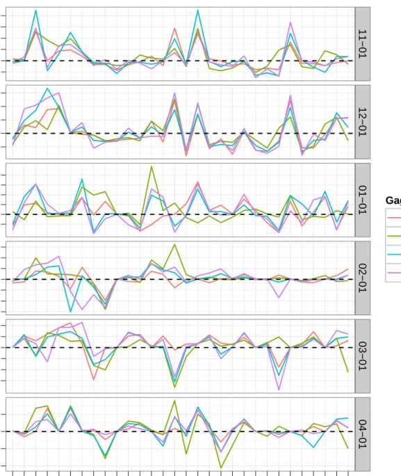
3.11 Yearly RPSS differences: positive values demonstrate improvement over ESP with
WG ESP and vice versa for negative . . . 72
3.12 Reliability diagram of April to July runoff above 10th percentile . . . 73
3.13 Reliability diagram of April to July runoff above 50th percentile . . . 74
3.14 Reliability diagram of April to July runoff above 90th percentile . . . 75
3.15 PDFs for 2005 runoff with vertical line showing 2005 value . . . 78
3.16 Same as Figure 3.15, but for 2006 . . . 79
3.17 RPSS for the conditional years . . . 81
3.18 Shifts in 2005 exceedance probabilities . . . 84
3.19 Same as Figure 3.18, but for 2006 . . . 85
A.1 Historical runoff volumes for sub-seasons . . . 100
A.2 April to July FRMN5 WG ESP vs ESP moments . . . 101
A.3 April to July NVRN5L WG ESP vs ESP moments . . . 102
A.4 April to May BFFU1 WG ESP vs ESP moments . . . 103
A.5 June to July BFFU1 WG ESP vs ESP moments . . . 104
A.6 April to May DRGC2 WG ESP vs ESP moments . . . 105
A.7 June to July DRGC2 WG ESP vs ESP moments . . . 106
A.8 April to May median and mean RPSS . . . 107
A.9 June to July median and mean RPSS . . . 108
A.10 April to May yearly RPSS differences (WG ESP - ESP) . . . 109
A.11 June to July yearly RPSS differences (WG ESP - ESP) . . . 110
A.12 RPSS of the two methods against observed April–July runoff, with unconditional
RPSS of the select years highlighted . . . 111
A.13 RPSS differences of the two methods (WG ESP - ESP) against observed April–July
runoff, with unconditional RPSS of the select years highlighted . . . 112
A.14 Correlations between ensemble mean and median values with historical April to July
runoff . . . 113
xiii
A.16 Reliability diagram of June to July runoff above 10th percentile . . . 115
A.17 Reliability diagram of April to May runoff above 50th percentile . . . 116
A.18 Reliability diagram of June to July runoff above 50th percentile . . . 117
A.19 Reliability diagram of April to May runoff above 90th percentile . . . 118
A.20 Reliability diagram of June to July runoff above 90th percentile . . . 119
A.21 April to July quantile-quantile plot for testing normality . . . 120
A.22 Same as Figure A.21 for April to May . . . 121
A.23 Same as Figure A.21 for June to July
. . . 122
A.24 April to May PDFs for 2005 runoff with vertical line showing 2005 value . . . 126
A.25 June to July PDFs for 2005 runoff with vertical line showing 2005 value . . . 127
A.26 Same as Figure A.24, but for 2006 . . . 128
A.27 Same as Figure A.25, but for 2006 . . . 129
A.28 April to July PDFs for 2005 runoff, not separated by lead time . . . 130
A.29 Same as Figure A.28, but for 2006 . . . 131
A.30 April to May RPSS for the conditional years . . . 132
A.31 June to July RPSS for the conditional years . . . 133
A.32 April to July 2005 QQ . . . 134
A.33 April to May 2005 QQ . . . 135
A.34 June to July 2005 QQ . . . 136
A.35 April to July 2006 QQ . . . 137
A.36 April to May 2006 QQ . . . 138
A.37 June to July 2006 QQ . . . 139
A.38 Shifts in 2005 exceedance probabilities (April to May) . . . 142
A.39 Same as Figure A.38, but for 2006 . . . 143
A.40 Shifts in 2005 exceedance probabilities (June to July) . . . 144
B.1 2005 IRI winter precipitation forecast . . . 147
B.2 2006 IRI winter precipitation forecast . . . 148
B.3 Distributional statistics of daily weather variables for ANB of 40:35:25 . . . 149
Chapter 1
Introduction
1.1
Background
Balancing competing demands of various water users in the western United States has proven
to be an ever-increasing challenge for water managers. Not only does the region have projected
population and economic growth, but the 2000’s drought,
1
climate variability, and climate change
further complicate planning and management. McCabe and Wolock (2009) (and references therein),
among others, have shown trends in warming since 1980 and general decrease in spring snowpack
throughout the western U.S. Rajagopalan et al. (2009) highlight the risk of reservoir depletion given
population growth and climate change, and suggest that flexibility be added to water management
practices. Studies referenced therein also predict that average annual flow will decline as a result
of climate change.
A majority of streamflow in the western U.S. originates from snowmelt. Whereas April 1st
snow water equivalent (SWE) as a predictor provides skillful predictions of late spring/early
sum-mer runoff, many critical management decisions are made months beforehand, even in November or
earlier. In the seven-state Colorado River Basin (CRB), the Colorado Basin River Forecast Center
(CBRFC) is the primary official provider of streamflow forecasts to water managing agencies such
as the U.S. Bureau of Reclamation and others. Currently the CBRFC and the Natural Resource
Conservation Service (NRCS) work together to create water supply outlooks in the CRB. Forecasts
are generated by each agency and subjectively combined into a joint, official-forecast (Hartmann
et al., 2002). NRCS uses a principle components regression (PCR) technique that primarily
re-lies on current snowpack and proxies of soil moisture such as antecedent streamflow and autumn
precipitation (Garen, 1992). At the seasonal time scale, CBRFC implements two techniques:
Sta-tistical Water Supply (SWS), a regression-based method that relates observed data (e.g., snow,
streamflow, precipitation) with future streamflow, and the model-based Ensemble Streamflow
Pre-diction (ESP). In conjunction with a physically based watershed model, ESP relies on historical
meteorological data as possible representations of the future; each historical year is then used to
simulate a streamflow trace (Day, 1985).
Ensemble forecasts have gained momentum in preference over deterministic forecasts, as
prob-abilistic forecasts have been found to be more “appropriate and articulate” (Pagano and Garen,
2005) and offer more skill and relative economic value than deterministic forecasts (Roulin, 2007;
Boucher et al., 2012). Ensemble forecasting is especially promising as the U.S. Bureau of
Recla-mation has developed the Mid-Term Operations Model (MTOM) (outlined in Grantz (2011) and
described in detail in Bracken (2011)). MTOM is an objective, ensemble-based operations model
where reservoir operations planning is engaged in a probabilistic mode. Having started running
in experimental mode in 2010, it is an upgrade of their “24-month study”, which helps anticipate
monthly inflow volumes to the major Reclamation-operated reservoirs in the Colorado Basin.
The ESP methodology has shortcomings in that the ensembles created are hindered by limited
historical data, which becomes even more limited with the addition of climatological forecasts
(forecast based on region). Improvements over ESP have been developed for short-to-medium
range (days-to-weeks) forecasting with the incorporation of ensemble weather forecasts (see Cloke
and Pappenberger (2009) for a review). As these weather forecasts come from numerical weather
models, their weather-scale reliability deteriorates after a medium-range, while their climate-scale
signals may still reduce uncertainty in ESP.
To improve upon ESP limitations, we propose the incorporation of climate-scale probabilistic
precipitation and temperature forecasts via the use of a hybrid nonparametric weather generator
to create a variety of weather sequences that are more skillful and comprehensive than those found
3
in a historical climatology. The approach is a multi-site, multi-variable generator based on
Api-pattanavis et al. (2007) and further developed as described in Chapter 2. Precipitation occurrence
is modeled with a two-state Markov chain and weather variables are selected using a k-nearest
neighbor (k-NN) resampling algorithm. The resulting weather sequences are run through a
water-shed model using the ESP framework to produce streamflow forecast ensembles (Chapter 3). This
weather generator can produce weather sequences that are unconditional or else conditioned on
climate forecasts from an arbitrary source. Unlike ESP, there is no limit to the number of traces
(i.e., size of ensemble) than can be generated to produce streamflow forecasts.
1.2
Study area and context
Our study was performed on the San Juan River Basin. With a drainage area of
approxi-mately 25,000 miles
2
, the San Juan River is the second largest tributary of the Colorado River and
runs a distance of 355 miles. The river flows from Colorado into New Mexico, then west to the
Colorado River and Lake Powell in Utah. Having an area near in size to West Virginia, drainage
areas are 39, 23, 20, and 17 percents in New Mexico, Colorado, Arizona, and Utah, respectively.
The San Juan river basin includes a wide range of elevations, from roughly 4000 ft before confluence
with the Colorado River, to above 14,000 ft in the San Juan Mountains. Climate zones range from
desert plateau to mountain forests. Winter snow and rain due to frontal storms and modest rains
from convective storms in summer are the main moisture input to the basin. Precipitation can vary
from above 60 inches annually in the mountain peaks, to below 10 inches in the desert plateau
2
.
Completed in 1962, the Navajo Reservoir dramatically altered the natural hydrograph of the
San Juan River. When filled, it occupies 15,610 acres, with a total capacity of 1.7 million acre-feet
(MaF) and an active capacity of 1.0 MaF.
3
Major tributaries above the dam are the Navajo,
Piedra, and Los Pinos Rivers. Of these only the Los Pinos is dammed (for agricultural purposes).
The Animas River is the major tributary below the Navajo Dam and is free flowing. A majority
2
http://www.usbr.gov/uc/wcao/rm/sjrip/
3
of the reservoir inflow occurs during the April-July runoff when an average of 0.66 MaF enter the
reservoir. Before damn construction, the gage at Bluff saw approximately 72% of the total annual
discharge occurring during that period (USBR, 2008).
Protecting natural ecology plays an important role in managing the San Juan. Tourism is
especially important to the basin economy as many anglers visit each year for the famous
abun-dance of rainbow trout. Fish such as the Colorado pikeminnow
(Ptychocheilus lucius)
and the
razorback sucker
(Xyrauchen texanus)
declined to endangered levels in the years after the Navajo
Reservoir was completed. Based on the recommended flows from joint research study of multiple
agencies (Holden, 1999), spring releases from the Navajo Reservoir must be a minimum of 250 cfs
and maximum controlled releases must be about 5000 cfs. Reservoir management must also take
into account other needs such as storing water for consumptive use, irrigation, flood control, and
generation of hydroelectric power. Finally, management of the San Juan River and the Navajo
Reservoir must meet agreed-upon flows as defined in the Upper Colorado River Basin Compact
and the Colorado River Compact.
1.3
Thesis outline
This thesis is written in manuscript form for the middle two chapters, which are self contained
sections in a format that is acceptable for submission to an academic journal. After this introductory
chapter, Chapter 2 describes the multisite stochastic weather generator. Then, Chapter 3 presents
the linkage of the weather generator with a physical model to produce streamflow forecasts. Chapter
4 provides overall conclusions and discussion for future work.
Chapter 2
Multisite Stochastic Weather Generation Using Cluster Analysis and K-nearest
neighbor Time Series Resampling
2.1
Introduction
Generation of synthetic weather sequences has been a topic of great interest in recent decades.
Since historical data is limited, these sequences are needed to drive process models of hydrology,
agriculture, erosion, ecology, construction delay, etc. (Wallis and Griffiths, 1997; Friend et al., 1997;
Eberle et al., 2002; Mountain and Jones, 2006; Leander et al., 2006, 2007; Caron et al., 2008), to
provide robust estimates of risks of decision variables, to enable better management of resources.
The generation is based on stochastic models fit to historic data hence commonly referred to as
stochastic weather generation. There is a rich literature on stochastic weather generators and the
traditional generators trace their origin to the Weather Generator Model (WGEN) of Richardson
(1981); Richardson and Wright (1984). In this, precipitation occurrence is modeled using Markov
chains (Richardson, 1981; Katz, 1977; Stern and Coe, 1984; Woolhiser, 1992) or as Poisson process
(Foufoula-Georgiou and Georgakakos, 1991; Furrer and Katz, 2008) and the amounts using
proba-bility density functions, such as two-parameter gamma (Katz, 1977; Buishand, 1978; Yang et al.,
2005; Furrer and Katz, 2007). Bivariate autoregressive models of first order lag are fit to model
maximum and minimum temperatures (Richardson, 1981). The models are fit for each month
to capture the seasonality. This method is also referred as parametric weather generators, given
the number of parameters of the various components. Generalized Linear Model (GLM) based
weather generators offer an alternative parametric approach to modeling daily weather (Chandler
and Wheater, 2002; Chandler, 2005; Furrer and Katz, 2007; Yang et al., 2005). In this the
precipita-tion and temperature are modeled as a series of GLMs with several covariates to capture seasonality,
lagged dependence etc. The flexible nature of GLMs enable the modeling of binary (precipitation
state) and continuous (precipitation intensity, maximum and minimum temperatures) variables
with mixed covariates. We refer the reader to Wilks and Wilby (1999) for a comprehensive review
of traditional parametric stochastic weather generators.
The above WGEN-based weather generators can be easily fit to daily weather at single
locations, but many applications, such as hydrologic, require daily weather at multiple locations
simultaneously. However, extending parametric models to multiple sites is not trivial. A major
disadvantage is that model parameters grow exponentially with number of locations and spatial
dependency also needs to be captured (Smith, 1994; Mehrotra et al., 2006). One such design (Wilks,
1998) involved a two-state, first-order Markov chain for precipitation occurrence and a mixed
exponential distribution for precipitation generation. Serially independent but spatially correlated
transformed normal variables enabled multisite generation; this was extended to additional weather
variables in Wilks (1999). Many subsequent parametric multisite rainfall generators have been
adaptations of the Wilks (1998) technique (Mehrotra et al., 2006; Brissette et al., 2007; Srikanthan
and Pegram, 2009) with further additional variations for temperature simulation (Qian et al., 2002;
Baigorria and Jones, 2010). Other multivariable methods involve disaggregating to individual
locations from a regionally developed model like a statistical downscaling model (Segond et al., 2006;
Mezghani and Hingray, 2009). Spatial models for rainfall occurrence and amounts using GLM for
individual sites and Latent Gaussian process to spatially interpolate the GLM parameters and thus
generate precipitation process in space, were developed by Kleiber et al. (2012). This approach has
the ability to incorporate maximum and minimum temperature to result in a parsimonious spatial
weather generator.
Nonparametric weather generators are an attractive alternative. Being data-driven, they can
capture deviations from standard probability distributions, as well as nonlinearities between
vari-ables. Past methods include kernel density estimators (Rajagopalan et al., 1997; Harrold et al.,
7
2003; Mehrotra and Sharma, 2007) and k-nearest neighbor (K-NN) bootstrapping (Brandsma and
Buishand, 1998; Rajagopalan and Lall, 1999; Buishand and Brandsma, 2001; Yates et al., 2003;
Beersma and Buishand, 2003; Sharif and Burn, 2007). The K-NN approach is increasing in
popu-larity due to its ease of implementation and effectiveness. In this, k-nearest neighbors are identified
to the weather vector on a current day ‘
t
’, from the historical data. Then one of these days is
resampled using a weight metric that gives most weight to the nearest neighbor and least to the
farthest. The uniformly distributed random number then resamples from these weighted days,
sim-ulating weather on day ‘
t
+ 1’. This is akin to simulating from the conditional probability density
function (PDF)
f
(
x
t
|
x
t
−
1
) with the PDF estimated locally in phase space. This method was first
introduced by Lall and Sharma (1996) and adopted for weather generation by Rajagopalan and
Lall (1999) and applied to different situations such as generating weather sequences conditioned on
climate change projections, for hydrologic forecasting etc. This approach was modified by
Apipat-tanavis et al. (2007) to a hybrid nonparametric model, where precipitation occurrence is modeled
with a two-state Markov chain and weather variables are selected using a K-NN resampling
algo-rithm. They also extended this to simulating weather sequences at multiple locations by applying
the K-NN bootstrap weather generator on the daily average weather time series over these
loca-tions. In this domain-aggregated, ‘da’, approach, the weather at all the locations is simulated by
resampling from the historical record at all locations on the same day, thereby maintaining spatial
correlations. Apipattanavis et al. (2007) demonstrated this with application to four locations in a
climatologically homogeneous region in northern Argentina.
Our motivation in this research comes from the need to generate daily weather sequences
at a large number of locations sprinkled over a heterogeneous watershed, to subsequently drive a
hydrologic modeling system to produce streamflow forecasts. The methodology of Apipattanavis
et al. (2007), based on resampling from a spatially averaged daily weather time series, may not
adequately capture the spatial nonhomogeneity. We propose a new adaptation to this approach
where the sites are (i) first clustered into homogeneous sub-regions based on historical seasonal
precipitation (or any other suite of attributes); (ii) a Markov chain is fit to cluster-averaged
pre-cipitation time series over the joint two-state, three-cluster (2
3
= 8 state) system to capture the
spatial correlation in the precipitation occurrence between the clusters; (iii) the K-NN bootstrap
is then applied to generate daily weather sequences conditioned on the precipitation state, for each
cluster. Thus, generating daily weather sequences at all the desired locations.
This weather generator has an additional feature where it can serve as a downscaling link
between probabilistic climate forecasts and hydrologic modeling. We investigate the proposed
methodology in the context of large-scale seasonal precipitation forecasts. With this option, the
conditioned generated weather sequences reflect prediction of wet or dry climate, which will then
result in wet or dry streamflow forecasts.
The paper is organized as follows. The application region and context are described along
with the data sets. The methodology is then described with the implementation. After
present-ing the results, we conclude with discussion of the methodology and potential applications and
improvements.
2.2
Study Region, Application Context and Data
With a drainage area of approximately 25,000 sq. miles, the San Juan River is the second
largest tributary of the Colorado River. Its area, nearly that of West Virginia, is approximately
split between New Mexico (39%), Colorado (23%), Arizona (20%), and Utah (17%). The San Juan
river basin includes a wide range of elevations, from roughly 4000-14,000 ft above sea level, and
climate zones, including desert and forest. DJF snow and rain due to frontal storms and modest
rains from convective storms in summer are the main moisture input to the basin. Precipitation
can vary from above 60 inches annually in the mountain peaks, to below 10 inches in the desert
plateau.
1
Prior to construction of the Navajo Dam, flows were snowmelt dominated, but with
reservoir operations, MAM runoff is stored and released during summer and later months (Holden,
1999).
1
9
Figure 2.1: San Juan Watershed: the four corners of Utah, Colorado, New Mexico, and Arizona is
just above the center of the figure
The Colorado Basin River Forecasting Center (CBRFC) provides ensemble seasonal
stream-flow forecasts at several lead times at multiple locations on the San Juan River. They use the
historic daily weather sequences to drive a physically based watershed model (Sacramento Soil
Moisture model, SAC-SMA). This generates as many ensemble members for the current forecast
season as the number of times the season appears in the historical record (Day, 1985). The historic
weather sequence thus provides a very limited set of ensembles. Ensembles are further reduced
when a seasonal forecast condition (e.g. “wet”) is imposed. Our proposed stochastic weather
gen-erator aims to solve this problem by simulating a rich variety of weather sequences over the study
domain.
The CBRFC divides the San Juan river basin in to 24 sub-basins (Figure 3.4) which are
further divided by elevation bands into two to three zones each, resulting in a total of 66 spatial
zones, or subcatchments. Based on observed historical data at weather stations scattered across
the basin, the CBRFC has created mean areal precipitation (MAP) and mean areal temperature
(MAT) for each zone at 6-hourly time steps.
2
These start in October of 1980 through September of
2010. From the 29 complete years, we calculate daily precipitation totals as well as daily minimum
and maximum temperatures which serve as inputs to our stochastic weather generator. We generate
100 ensemble members of daily weather sequences for all 66 zones over the 29 year period. These
weather ensembles will be applied in future studies to drive a watershed model and to robustly
estimate streamflow probabilities at various points in the basin as well as management risks. In
this study, we evaluate our weather generator approach against the observed, seasonal statistics of
daily MAP and MAT timeseries.
2.3
Methodology
2.3.1
Cluster Analysis
To parse spatial inhomogeneity of weather over our domain, we employ K-means cluster
analysis (Everitt, 1979), with clustering on seasonal precipitation totals. The objective is to classify
M
= 66 points in
N
= 29 years dimensions into
k
clusters such that the within sum of squares
(WSS) over all clusters is minimized without over-fitting the clustering (i.e., using too high a
k
).
The Hartigan-Wong approach algorithm is employed (Hartigan and Wong, 1979). Because
initial centroids are selected at random, clustering is repeated 50 times to investigate uncertainty
in WSS for each choice of
k
. Our ‘kink plot’ (Figure 2.2) shows WWS and its 50% (boxes) and
90% (whiskers) uncertainty over 50 clustering trials as a function of k, the number of clusters. The
kink, or decrease in the reduction of WSS with increasing number of clusters, indicates the optimal
number of clusters (e.g. Hastie et al. (2009)).
2
11
2.3.2
Spatial Precipitation Occurrence Model
The domain-aggregate (‘da’) weather generation approach of Apipattanavis et al. (2007)
models temporal precipitation occurrence via a 2-state Markov chain with states “wet” and “dry.”
The region is wet (dry) if its domain average precipitation is above (below) 0.1 inches. The 2
2
elements (
p
dd
, p
dw
, p
wd
, p
ww
) of the transition probability matrix (TPM) are estimated using
maxi-mum likelihood. In the domain aggregate approach, Markov transition probabilities are calculated
on domain averaged weather at each time step. We compute the Markov transition probabilities
for each month separately within each season.
Described in the following section, the Markov modeled state conditions selection of a
his-torical weather observation under K-NN resampling. The problem with this method is that daily
precipitation and temperature over multiple locations become more heterogeneous as the domain
size grows. The use of domain average precipitation becomes inappropriate for estimating the
domain-wide precipitation state and thus for both calculation of state transition probabilities and
for selecting nearest neighbors from the historical record. Domain-averaged weather is also used in
the K-NN resampling scheme described below. By clustering simulations by total seasonal
precip-itation within the domain, we aim to resolve the large-scale, spatial heterogeneity problem of the
‘da’ approach.
After identifying
k
clusters based on seasonal precipitation totals within the spatial domain,
the simplest approach is to directly model the clusters individually and independently using the
‘da’ approach in each cluster separately. We term this approach ‘ca’ for cluster-aggregate. Because
our application is hydrologic response, with future consideration of the basin outlet, ‘ca’ has the
obvious shortcoming that the upstream weather inputs are not coordinated.
We explore two solutions to this problem. First, in order to coordinate (or correlate)
basin-wide response, we propose generating the precipitation state over the full domain as in the ‘da’
approach and then using this global state within each cluster to condition selection of observed
weather from the within-cluster historical record. Deemed ‘caShared’, this approach may suffer
from the obvious deficiency that gross heterogeneities over the domain at the cluster level will not
be appropriately modeled. For example, if it tends to rain in one cluster while others are dry, then
this situation will be undersimulated.
Second, we take a more nuanced approach to the problem of spatial coordination of cluster
states by modeling Markov transition probabilities between all possible states of the three cluster
system. If
N
s
is number of precipitation states and
k
the number of clusters, then say for
k
= 3
clusters there are 8 possible states.
N
s
k
= 8 =
ddd, ddw, dwd, dww, wdd, wdw, wwd, www
(2.1)
We term this approach ‘caJoint’. The probability of transitioning to any joint state can be
com-puted using cluster-average precipitation and the established threshold of 0.1 inches to determine
“wet”. Calculating the joint transition probability begins with cluster-average precipitation and
the previous, two-state threshold of 0.1 inches to distinguish wet from dry. We compute the Markov
transition probabilities for each month separately based on the historical transitions between the
resulting 8 states of the system. For our simple,
k
-cluster system, the transition probability matrix
is 8 x 8 when
k
= 3 (though all transitions may not actually occur in the data). Note that even for
a two state, four cluster system the number of distinct transition probabilities is already 16 x 16.
One may employ any number of states and clusters, but the complexity can rapidly increase when
modeling the joint states of the system as proposed here.
2.3.3
K-NN Resampling
For all of the above approaches (‘da’, ‘ca’, ‘caShared’, and ‘caJoint’), daily weather sequences
at all locations are generated using the algorithm of Apipattanavis et al. (2007). The basic idea
is, for a given day
t
, to sample areal-averaged weather vectors from the conditional PDF,
f
(
x
t
|
DOY, x
t
−
1
, S
t
−
1
, S
t
), of areal-averaged weather vectors,
x
t
, given the day of year, DOY, yesterday’s
simulated weather,
x
t
−
1
, yesterday’s precipitation state,
S
t
−
1
, and today’s precipitation state,
S
t
.
13
at each location in the region is used in the simulation. The cluster-based approaches have three
regions, and so three potentially different days will be selected from the record, corresponding to
each region, to simulate the locations in each.
Given an initial area-average weather vector, the historical areal-average weather vectors,
and the previously generated sequence of areal-averaged precipitation states for some area, the
following algorithm applies to all approaches (‘da’ and cluster based):
(1) A 7-day window centered on the day of year for time
t
in the simulated sequence filters out
the remainder of the historical record (
|
DOY
).
(2) Days within this window with matching, areal-averaged state transitions to simulated day
t
−
1 are extracted (
|
S
t
−
1
, S
t
).
(3) Each areal-averaged weather variable within the selected days is scaled by the reciprocal
of its historical standard deviation on day
t
−
1 to provide equal weight over all variables
in the next step.
(4) Euclidean distances are calculated between all candidate weather vectors over the region
and the previously simulated weather vector on day
t
−
1.
(5) The most similar (closest) weather vectors are limited to a neighborhood of size
K
=
√
N
,
where
N
is the length of the dataset (Lall and Sharma, 1996).
(6) These
K
nearest neighbors are assigned a probability using a discrete decreasing kernel
p
(
i
) =
P
K
1
/i
j
=1
1
/j
(2.2)
(Lall and Sharma, 1996; Rajagopalan and Lall, 1999), where
p
(
i
) is the probability that
the
i
th neighbor will be selected, thus giving the
k
th neighbor the lowest probability.
(7) A neighbor (i.e., a historical day) is randomly resampled according to these weights.
(8) Its
successive
day in the historical record is selected as the weather on day
t
and represents
all locations in the modeled area.
This algorithm is repeated for each day in the desired simulation period. Table 2.1
demon-strates the selection of nearest neighbors for a window centered on December 9th.
2.3.3.1
Conditional Resampling
Synthetic weather sequences are often required that are consistent with large-scale, seasonal
climate forecasts. We incorporate the seasonal precipitation forecasts issued by the International
Research Institute for Climate and Society
3
into our methodology. These give the probability of
each seasonal precipitation tercile, above:normal:below (ANB). The approaches of Apipattanavis
et al. (2007) and Yates et al. (2003) to conditional resampling based on climate forecasts is to
modify the weights in step 6 of the K-NN resampling algorithm. Because we found this approach
to only mildly modify the outcome, we propose a new strategy here.
(1) Calculate seasonal precipitation totals in each year and associate it with each day in a given
season.
(2) Follow the K-NN algorithm through step 2: find all historical days in the 7-day moving
window which match the simulated transitions, which we will call
T
.
(3) Now the neighborhood of size
K
=
√
N
is no longer determined by euclidean distances
(replacing steps 3 through 5).
(4) Then for a wet (dry) ANB
(a) Sort the matching days,
T
, based on decreasing (increasing) seasonal totals.
(b) The nearest (farthest) neighbors are
A
×
K
of head (tail) of
T
.
(c) The farthest (nearest) neighbors are
B
×
K
of tail (head) of
T
.
(d) What remains is filled by
N
×
K/
2 on either side of the median seasonal total of
T
.
(5) Resume step 6 from the algorithm above.
3
15
This method ensures preferential treatment of seasons that have desirable characteristics.
Since daily precipitation intensities are not necessarily sorted in order of highest or lowest,
resam-pling is not too severely modified and a variety of weather scenarios is still maintained. Table
2.2 demonstrates how the
K
neighbors are determined for an ANB of 65:25:10. With
K
= 14,
0
.
65
×
K
= 9, thus the neighborhood from 1 to 9 is filled from the 9 highest totals according to the
sorted
T
. As 0
.
1
×
K
= 1, the last member of the neighborhood is filled by the day corresponding
to the lowest value in sorted
T
. The remaining values are filled by days falling on either side of
the median. In the unconditional simulation example (Table 2.1), the weather on December 12,
2007 was determined as the 8th nearest neighbor. For the wet simulation (Table 2.2), it became
the nearest neighbor because of its corresponding seasonal totals, and thus is more likely to be
sampled.
Table 2.1:
K
-nearest neighbors for ordinal day of December 9th: unconditional simulation
year
month
day
p
tmin
tmax
seq
state
trans
total
1
2000
12
9
0.12
-3.63
2.36
7278
w
w2d
6.58
2
1996
12
11
0.39
-1.20
3.58
5820
w
w2d
8.80
3
1991
12
11
0.71
-7.10
1.05
3995
w
w2d
5.37
4
1997
12
8
0.38
-6.76
-0.85
6182
w
w2d
5.02
5
1993
12
12
0.44
-6.49
0.02
4726
w
w2d
4.91
6
1996
12
7
0.14
-9.89
3.46
5816
w
w2d
8.80
7
1998
12
6
0.15
-11.62
-4.44
6545
w
w2d
3.08
8
2007
12
11
0.37
-7.12
-1.18
9835
w
w2d
14.77
9
2006
12
11
0.24
-8.11
-0.17
9470
w
w2d
5.19
10
2003
12
8
0.30
-5.75
0.91
8372
w
w2d
6.71
11
1982
12
9
0.51
-4.41
2.84
708
w
w2d
6.33
12
1982
12
11
0.11
-3.94
1.00
710
w
w2d
6.33
13
1985
12
10
0.21
-14.11
-4.86
1804
w
w2d
4.29
14
1984
12
8
0.43
-7.64
3.11
1437
w
w2d
7.76
Table 2.2: Same as Table 2.1, but for wet simulation with ANB of 65:25:10
year
month
day
p
tmin
tmax
seq
state
trans
total
1
2007
12
11
0.37
-7.12
-1.18
9835
w
w2d
14.77
2
1996
12
7
0.14
-9.89
3.46
5816
w
w2d
8.80
3
1996
12
11
0.39
-1.20
3.58
5820
w
w2d
8.80
4
2008
12
8
0.26
-3.05
1.79
10197
w
w2d
8.68
5
1984
12
8
0.43
-7.64
3.11
1437
w
w2d
7.76
6
1994
12
6
0.88
-2.51
2.06
5085
w
w2d
7.00
7
2003
12
8
0.30
-5.75
0.91
8372
w
w2d
6.71
8
1986
12
6
0.70
-3.75
3.06
2165
w
w2d
6.68
9
2000
12
9
0.12
-3.63
2.36
7278
w
w2d
6.58
10
1982
12
9
0.51
-4.41
2.84
708
w
w2d
6.33
11
1982
12
11
0.11
-3.94
1.00
710
w
w2d
6.33
12
2009
12
8
0.83
-13.20
-3.25
10562
w
w2d
6.28
13
1991
12
11
0.71
-7.10
1.05
3995
w
w2d
5.37
14
2001
12
11
0.11
-10.68
-1.42
7645
w
w2d
1.91
2.4
Results
Cluster analysis was performed on seasonal precipitation totals, separately for each three
month season, Dec–Feb (DJF), Mar–May (MAM), Jun–Aug (JJA) and Sep–Nov (SON). Based on
the kink plot for DJF (Figure 2.2) three clusters were chosen to be the optimal number, similarly
for other seasons. Boxplots of elevations of the locations falling in each cluster are shown in Figures
2.3 and 2.4 — it can be seen that the clusters fall quite well along the elevations. In that, all the
high elevation locations are together in cluster ‘a’, the middle elevations in cluster ‘b’ and the lower
in ‘c’. This is consistent in that the DJF precipitation has a distinct elevation signal, with higher
elevation regions receiving more snow and vice-versa. This is found to be the case in all the seasons
except for summer where the precipitation is less organized by elevation, as would be the case with
17
convective nature of precipitation in this season. The number of locations in each cluster in each
season is shown in Table 2.3. The spatial state simulation and K-NN resampling are applied to
locations in each cluster to generate daily weather sequences.
●
●
●
●
●
●
●
●
●
●
●
●
●
●
●
●
●
●
●
●
●
●
●
●
●
●
●
●
●
●
●
●
●
●
●
●
●
●
●
●
●
●
●
●
●
●
●
●
●
●
●
●
●
●
●
●
●
●
●
●
●
●
●
●
●
●
●
●
●
●
●
●
●
●
●
●
●
●
●
●
●
●
●
●
●
●
●
●
●
●
●
●
●
●
●
●
●
●
●
●
●
●
●
●
●
●
DJF
JJA
MAM
SON
5000
10000
15000
20000
5000
10000
15000
20000
1
2
3
4
5
6
7
8
9 10
1
2
3
4
5
6
7
8
9 10
K
Within cluster sum of squares
Figure 2.2: Uncertainty in the within sum of squares (WSS) as a function of
k
th for 50 independent
clusterings of total seasonal precipitation over 66 stations in 29 years.
2.4.1
Clusters
Classification of ‘a’, ‘b’, or ‘c’ correspond to cluster groupings with highest, middle, and
lowest median elevations, respectively in each season. Assignment of subcatchments within groups
will change with each analysis due to the heuristic nature of the algorithm. However, as very little
change in WSS is seen in Figure 2.2 for
k
= 3, the results are assumed as stable.
Table 2.3: Number of stations falling within each cluster
a
b
c
DJF
17
26
23
MAM
19
25
22
JJA
22
22
22
SON
17
26
23
Boxplots in Figures 2.3a and 2.4a depict elevations of subcatchment centroids organized by
cluster groups. Though clustering was performed on precipitation, this shows there is a heavy
correlation with elevation as well. DJF is more organized by elevation while summer has more
influence from spatial proximity. Figures 2.3b and 2.4b show cluster ‘a’ predominantly falls within
forested, mountainous areas while ‘c’ falls in low-lying arid regions. Cluster ‘b’ has a mix of
characteristics from the other two groups. Cluster medians change appreciable with season. Cluster
‘c’ is the most stable of the groupings—its member population remains relatively consistent between
the seasons and its median elevation stays near 6500 ft. Conversely ‘a’ and ‘b’ have more variable
member numbers and the median elevations can change up to 1000 ft between seasons.
Figure 2.5 displays between-cluster correlations in the observed record and illuminates the
motivation behind the ‘caShared’ and ‘caJoint’ methodologies. From these figures it is evident that
each cluster cannot be assumed as independent from others, thus they should not be simulated
independently, as in the ‘ca’ approach shown below.
19
6000
7000
8000
9000
10000
11000
●
●
●
●
●
●
●
●
●
●
●
●
●
●
●
●
●
●
●
●
●
●
●
●
●
●
●
●
●
●
●
●
●
●
●
●
●
●
●
●
●
●
●
●
a
b
c
Cluster
Ele
v
ation (f
eet)
Elevation
●
●
●
●
●
●
●
11500
10500
9500
8500
7500
6500
5500
Cluster
●
●
a
b
c
(a)
35.5
36.0
36.5
37.0
37.5
●
●
●
●
●
●
●
●
●
●
●
●
●
●
●
●
●
−110.0
−109.5
−109.0
−108.5
−108.0
−107.5
−107.0
−106.5
Longitude
Latitude
Elevation
●
●
●
●
●
●
●
11500
10500
9500
8500
7500
6500
5500
Cluster
●
a
b
c
(b)
6000
7000
8000
9000
10000
11000
●
●
●
●
●
●
●
●
●
●
●
●
●
●
●
●
●
●
●
●
●
●
●
●
●
●
●
●
●
●
●
●
●
●
●
●
●
●
●
●
●
●
●
●
●
●
●
●
●
●
●
●
●
●
a
b
c
Cluster
Ele
v
ation (f
eet)
Elevation
●
●
●
●
●
●
●
11500
10500
9500
8500
7500
6500
5500
Cluster
●
●
a
b
c
(a)
35.5
36.0
36.5
37.0
37.5
●
●
●
●
●
●
●
●
●
●
●
●
●
●
●
●
●
●
●
●
●
●
−110.0
−109.5
−109.0
−108.5
−108.0
−107.5
−107.0
−106.5
Longitude
Latitude
Elevation
●
●
●
●
●
●
●
11500
10500
9500
8500
7500
6500
5500
Cluster
●
a
b
c
(b)
21
2.4.2
Unconditional Simulation
We first evaluate characteristics of the four methodologies against the observed statistics of
the seasonal precipitation. Figure 2.6 compares probability density functions (PDF) of basin total
seasonal precipitation for the four methods along with the historical PDF. With a lack of
inter-cluster dependency in the ‘ca’ method, its PDF tends towards the mean with a thin tail behavior
in all seasons. In DJF and MAM, the other three methods are similar to each other and closer to
the historical distribution. All four seasons reinforce the conclusion drawn from Figure 2.5 that
independence cannot be assumed between clusters.
Figure 2.7 shows simulated versus observed average number of wet day occurrences per season.
It is evident that forcing the same precipitation state across the clusters in the ‘caShared’ method
oversimulates the number of wet days in the lower elevation clusters and undersimulates in the
higher elevation for all seasons. Thus ‘caShared’ does not appear like a viable option. The other
three methods are near-similar in their performance and have
R
2
values of 0.99 with the observed.
Figure 2.8 divides Figure 2.6 into within-cluster total seasonal precipitation, showing the
PDFs for each cluster. The cluster division, ‘ca’ now has a strong performance as it simulates
each cluster independently thus reproducing individual cluster distributions, whereas it performed
poorly on the basin-wide precipitation (Figure 2.6). The ‘caShared’ method seems to oversimulate
in the lower elevation clusters (b and c) and undersimulates in the high elevation cluster (a),
similar to the behavior in Figure 2.7. With the exception of summer, ‘da’ and ‘caJoint’ exhibit
good performances in terms of capturing the observed PDF.
ab
bc
ac
0
20
40
60
80
100
0
20
40
60
80
100
0
20
40
60
80
100
0
20
40
60
80
100
DJF
MAM
JJ
A
SON
0.0 0.2 0.4 0.6 0.8 1.0
0.0 0.2 0.4 0.6 0.8 1.0
0.0 0.2 0.4 0.6 0.8 1.0
Pearson correlation coefficient
Count
(a) Precipitation
ab
bc
ac
0
50
100
150
200
0
50
100
150
200
0
50
100
150
200
0
50
100
150
200
DJF
MAM
JJ
A
SON
0.6 0.7 0.8 0.9 1.0
0.6 0.7 0.8 0.9 1.0
0.6 0.7 0.8 0.9 1.0
Pearson correlation coefficient
Count
(b) Max temperature
ab
bc
ac
0
50
100
150
0
50
100
150
0
50
100
150
0
50
100
150
DJF
MAM
JJ
A
SON
0.5 0.6 0.7 0.8 0.9 1.0
0.5 0.6 0.7 0.8 0.9 1.0
0.5 0.6 0.7 0.8 0.9 1.0
Pearson correlation coefficient
Count
(c) Min temperature
Figure 2.5: Histograms of between-cluster correlations in the observed data for all stations in each
pair of clusters
23
DJF
MAM
JJA
SON
0.001
0.002
0.003
0.004
0.001
0.002
0.003
0.004
0.001
0.002
0.003
0.004
0.005
0.0005
0.0010
0.0015
0.0020
0.0025
0.0030
0
200
400
600
800
1000
0
200
400
600
800
200
400
600
800
0
200
400
600
800
Precipitation total (inches)
Probability density
Method
da
ca
caShared
caJoint
observations
●
●
●●
●
●
●
●
●
●
●
●●
●
●
●●
●
●
●
●
●
●
●
●
●
●
●
●
●
●
●
●
●
●
●
●
●
●
●
●
●
●
●
●
●
●
●
●
●
●
●
●
●
●
●
●
●
●
●
●
●
●
●
●
●
●
●
●●
●
●
●
●
●
●
●
●●
●
●
●●
●
●
●
●
●
●
●
●
●
●
●
●
●
●
●
●
●
●
●
●
●
●
●
●
●
●
●
●
●
●
●
●
●
●
●
●
●
●
●
●
●
●
●
●
●
●
●●
●
●
●
●●
●
●
●
●
●
●
●
●●
●
●
●●
●
●
●
●
●
●
●
●
●
●
●
●
●
●
●
●
●
●
●
●
●
●
●
●
●
●
●
●
●
●
●
●
●
●
●
●
●
●
●
●
●
●
●
●
●
●
●●
●
●
●
●●
●
●
●
●
●
●
●
●●
●
●
●●
●
●
●
●
●
●
●
●
●
●
●
●
●
●
●
●
●
●
●
●
●
●
●
●
●
●
●
●
●
●
●
●
●
●
●
●
●
●
●
●
●
●
●
●
●
●
●
●
●
da
ca
caShared
caJoint
10
15
20
25
10
15
20
25
10
15
20
25
10
15
20
25
Observed average wet days per season
Sim
ulated a
v
er
age w
et da
ys per season
Cluster
●
●
●
a
b
c
(a) DJF
●
●
●
●●
●
●
●
●
●
●
●
●
●
●
●
●
●
●
●
●
●
●
●
●
●
●
●
●
●
●
●
●
●
●
●
●
●
●
●
●
●●
●
●
●
●
●
●
●
●
●
●
●
●
●
●
●
●
●
●
●
●
●
●
●
●
●
●
●
●
●
●
●
●
●
●
●
●
●
●
●
●
●
●
●
●
●
●
●
●
●
●
●
●
●
●
●
●
●
●
●
●
●
●
●
●
●●
●
●
●
●
●
●
●
●
●
●
●
●
●
●
●
●
●
●
●
●
●
●
●
●
●
●
●●
●
●
●
●
●
●
●
●
●
●
●
●
●
●
●
●
●
●
● ●
●
●
●
●
●
●
●
●
●
●
●
●
●
●
●
●
●●
●
●
●
●
●
●
●
●
●
●
●
●
●
●
●
●●
●
●
●
●
●
●
●
●
●
●
●
●
●
●
●
●
●
●
●
●
●
●
●
●
●
●
●
●
●
● ●
●
●
●
●
●
●
●
●
●
●
●
●
●
●
●
●
●●
●
●
●
●
●
●
●
●
●
●
●
●
●
●
●
●
●
●
●
●
●
●
●
da
ca
caShared
caJoint
5
10
15
20
25
5
10
15
20
25
10
15
20
25
10
15
20
25
Observed average wet days per season
Sim
ulated a
v
er
age w
et da
ys per season
Cluster
●
●
●
a
b
c
(b) MAM
●
●
●
●
●
●
●
●
●
●
●
●
●
●
●
●●●
●
●
●●
●
●
●
●
●
●
●
●
●●
●
●
●
●
●
●
●
●
●
●
●
●
●
●
●
●
●
●
●
●
●
●
●
●
●
●
●
●
●
●
●
●
●
●
●
●
●
●
●●
●
●
●
●
●
●
●
●
●
●●●
●
●
●●
●
●
●
●
●
●
●
●
●
●
●
●
●
●
●
●
●
●
●
●
●
●
●
●
●
●
●
●
●
●
●
●
●
●
●
●
●
●
●
●
●
●
●
●
●
●
●
●
●●
●
●
●
●
●
●
●
●
●
●●●
●
●
●●
●
●
●
●
●
●
●
●
●
●
●
●
●
●
●
●
●
●
●
●
●
●
●
●
●
●
●
●
●
●
●
●
●