International Journal of Business,Economics and Management Works
Kambohwell Publisher EnterprisesISSN: 2410-3500 Vol. 4, Issue 11, PP. 1-5, November 2017 www.kwpublisher.com
Selection of Best ARIMA Modeling Approach for Forecasting Time
Series Patterns; A Case Study on Colombo Stock Exchange
Madushani M.L.P*, Erandi M.W.A*, Madurangi L.H.L.S*, Sivaraj L.B.M*,
Weerasinghe W.D .D*, R.M KapilaTharangaRathnayaka
Abstract—Stock market indexes provide a yardstick with which investors can compare the performance of their individual stock portfolios. The propose of this paper is to examine a suitable model for forecasting stock prices under the volatility in the Colombo Stock Exchange (CSE), Sri Lanka.
Since the data has a non-seasonal linear trend, an autoregressive integrated moving average model has used for modeling and forecasting. The results suggested that ARIMA model is more suitable for forecasting ASPI index under the volatility.
Keywords—Modeling, Stock exchange, ARIMA
I. BACKGROUND TO THE STUDY
A stock market is a place where facilitate exchange of securities between buyers and sellers (virtual or real) in a single platform. Generally, the movements of the stock prices are highly volatile and make much more dynamics. So, day by day the large number of companies has been listed on stock exchanges across the world.
In a trading manner, the forecasting and analyzing is the most significant process that helps to judge the market risk and grab scarce opportunities; especially, forecasting the direction of the index or stock price for the next day is much more important for speculators and investors. So this study mainly focuses to propose a suitable methodology for forecasting stock prices under the volatility.
According to the literature, different type of methodologies can be seen for forecasting stock price indices. Jinchuan et.al (2008) and Rathnayaka et.al (2014 and 2015) were carried out different type of studies to forecast Stock Market Volatility using different type of ARCH methodologies; especially, GARCH-M model was used to test the long-term volatility
self-similarity and the correlation between risk and return;
TGARCH model was introduced to test the volatility leverage effect; EGARCH model was applied to verify the asymmetry heteroscedasticity of stock price fluctuation. Based on the empirical findings, Jinchuan et.al (2008) has suggested that the China bull market implies a high uncertainty and risk in upcoming two years.
According to the Ayodele et.al (2014), ARIMA models can be compete reasonably well with emerging forecasting techniques in short-term predictions. Based on the published stock data was obtained from New York Stock Exchange (NYSE) and Nigeria Stock Exchange (NSE), Ayodele et.al (2014) have done price predictive model development for stock forecasting’s. According to the performances comparisons based on the their Duane model and ARIMA models, ARIMA model is a viable alternative that gives satisfactory results in terms of its predictive performances.
The current study was carried out based on Colombo Stock Exchange (CSE), Sri Lanka. The CSE is a mutual exchange and has 15 full members and 13 trading members licensed to trade both equity and debt securities. As of 31 July 2014, 295 companies are listed on the CSE, representing twenty business sectors with a market capitalization over 2.4 trillion rupees (over US$18.5 billion), which corresponds to approximately 1/3 of the Gross Domestic Product of the country. ("Colombo Stock Exchange (CSE) | Colombo Stock Watch", 2016)
Generally, the two Price indices are mainly running under the CSE. They are; the All Share Price Index (ASPI) and the S&P Sri Lanka 20 Index (S&P SL20). ASPI measures the movement of share prices of all listed companies. It is based on market capitalization where, the weighting of shares is conducted in proportion to the issued ordinary capital of the listed companies, valued at current market capitalization.
The propose of this study is to examine a suitable model for forecasting stock prices under the volatility in the Colombo Stock Exchange (CSE), Sri Lanka. The rest of the paper is organized as follows. Section II develops the hypothesis and explains the methodology used in our study. Section III briefly presents the experimental results including results and ends up with the conclusion and future work in Section V.
Madushani M.L.P*, Erandi M.W.A*, Madurangi L.H.L.S*, Sivaraj L.B.M*, Weerasinghe W.D .D*: Department of Statistics & Computer Science, Faculty of Science, University of Kelaniya, Sri Lanka.
R.M KapilaTharangaRathnayaka: Faculty of Sciences, Sabaragamuwa University of Sri Lanka,Sri Lanka, [email protected]
II. METHODOLY
There are several different approaches have been seen in time series modeling and forecasting. Traditional statistical models include moving average, exponential smoothing, and ARIMA which are constrained to be linear functions to use predictions based on past observations. Because of their relative simplicity in understanding and implementation, linear models have been the main research focuses and applied tools during the past few decades.
In this section, we focus on the basic principles and modeling process of the ARIMA model under the three different steps as follows.
A. Step -1; Test of Stationary
First, confirm Generally, the financial data are non-seasonal and highly fluctuate over the time. Hence, test for the stationary and non-stationary conditions is the initial step to be carryout. The concept of stationary of a stochastic process can be visualized as a form of statistical equilibrium. The statistical properties such as mean and variance of a stationary process do not depend upon time. It is a necessary condition for building a time series model that is useful for future forecasting. Further, the mathematical complexity of the fitted model reduces with this assumption.
There are two types of stationary processes which have defined in literature. A process { Y(t),t = 0,1, 2,...} is strongly Stationary or Strictly Stationary if the joint probability distribution function of {Yt−s,Yt−s+1,...,Yt,...Yt+s−1,Yt+s} is independent of t for all s. Thus for a strong stationary process the joint distribution of any possible set of random variables from the process is independent of time. However, for practical applications, the assumption of strong stationary is not always needed (Tsay, 2005).
It is important to note that neither strong nor weak stationarity implies the other. However, a weakly stationary process following normal distribution is also strongly stationary. Some mathematical tests like the one given by Dickey and Fuller are generally used to detect stationarity in a time series data (Tsay, 2005).
According to the past studies Augmented Dickey-Fuller test (ADF) and Phillips-Perron test (PP) are the widely used techniques for the identification of the presence of unit roots. If the null hypothesis (dataset has a unit root) not being rejected for the original dataset then we take the differenced data and do the same procedure. According to at which differenced the dataset being stationary, determine the value of parameter d in the ARIMA model. However for relatively short time span, one can reasonably model the series using a stationary stochastic process. Usually time series, showing trend or seasonal patterns are non-stationary in nature. In such cases, differencing and power transformations are often used to remove the trend and to make the series stationary.
.
B. Step 2: Fitting suitable ARIMA (p, d, q) model
In an autoregressive integrated moving average model, the future value of a variable is assumed to be a linear function of several past observations and random errors. That is, the underlying process that generate the time series has the form. 𝒚𝒕= 𝜽𝟎+ ∅𝟏𝒚𝒕−𝟏+ ⋯ ∅𝒑𝒚𝒕−𝒑+ 𝜺𝒕− Ɵ𝟏ɛ𝒕−𝟏… − Ɵ𝒒ɛ𝒕−𝒒(1) where yt and ɛt are the actual value and random error at time
period t, respectively; ϕi (i = 1,2,…p) and θj (j = 0,1,2,...q) are
model parameters. p and q are integers and often referred to as orders of the model. Random errors, ɛt, are assumed to be
independently and identically distributed with a mean of zerand a constant variance of σ2.
Above equation (1) entails several important special cases of the ARIMA family of models. If q = 0, then (1) becomes an AR model of order p. When p = 0, the model reduces to an MA model of order q.
Based on the earlier work of Yule and Wold, Box and Jenkins developed a practical approach to building ARIMA models, which has the fundamental impact on the time series analysis and forecasting applications. This three-step model building process is typically repeated several times until a satisfactory model is selected. The final selected model can then be used for prediction purposes. The Box-Jenkins forecast method is schematically being shown below.
Figure 1: Model Approach Process
Finally, Forecasting performance of the various types of ARIMA models would be compared by computing statistics like Akaike Information Criteria (AIC), Schwartz Bayesian Criterion (SBC) and Hannan-Quinn Criterion (HQC). On the basis of these aforementioned selection and evaluation criteria concluding remarks have been drawn.
III. RESULTS AND DISCUSSION
A. Case study: CSE
The current study was carried on secondary data which were used to demonstrate the behavior of the Colombo Stock Exchange, Sri Lanka. Monthly trading data of two main price indices namely All Share Price Index (ASPI) and S&P Sri Lanka 20 Price Index (SL20) from January 2005 to September 2016 and June 2012 to August 2016 were used respectively.
Since the stock exchange depends on time, the researchers tend to fit time series models to examine the behavior of the stock exchange. Figure 2 and Figure 3 represent the time series plot for ASPI and SL20 respectively. According to both plots of time series, significant trend can be seen for ASPI and SL20 respectively.
Figure 2: Time series plot of ASPI values from January 2005 to September 2016
B. Abbreviations and Acronyms
As an initial step, two stationary mathematical methods namely Augmented Dickey Fuller (ADF) test and Phillips–Perron (PP) test were used to test the following hypothesis.
H0: Time series has a unit root H1: Time series has not a unit root
According to the summarized results in Table 1, both tests clarified that the observable time series are not stationary. So, as a next step, data transformation has to be done to make the time series stationary. Therefor 1st differenced of both indices were considered and carried out same study again. Both test results confirmed that the 1st differenced time series of ASPI and SL20 are stationary under the 0.05 level of significance.
Figure 3: Time series plot of SL20 values from June 2012 to August 2016
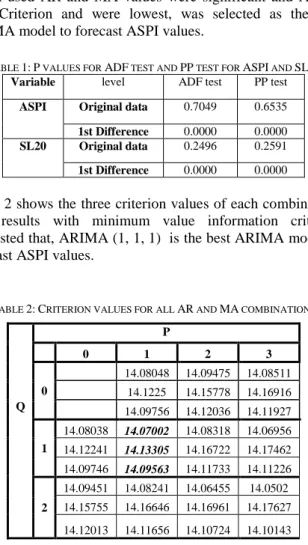
C. Possible parameter values for ARIMA (PIQ) model According to the tails off position of PACF plot of AR and MA values from 0 to 3 would be most significant. Model in which used AR and MA values were significant and Akaike Info Criterion and were lowest, was selected as the best ARIMA model to forecast ASPI values.
TABLE 1:P VALUES FOR ADF TEST AND PP TEST FOR ASPI AND SL20
Variable level ADF test PP test
ASPI Original data 0.7049 0.6535
1st Difference 0.0000 0.0000
SL20 Original data 0.2496 0.2591
1st Difference 0.0000 0.0000
Table 2 shows the three criterion values of each combination. The results with minimum value information criterion suggested that, ARIMA (1, 1, 1) is the best ARIMA model to forecast ASPI values.
TABLE 2:CRITERION VALUES FOR ALL AR AND MA COMBINATIONS
Q P 0 1 2 3 0 14.08048 14.09475 14.08511 14.1225 14.15778 14.16916 14.09756 14.12036 14.11927 1 14.08038 14.07002 14.08318 14.06956 14.12241 14.13305 14.16722 14.17462 14.09746 14.09563 14.11733 14.11226 2 14.09451 14.08241 14.06455 14.0502 14.15755 14.16646 14.16961 14.17627 14.12013 14.11656 14.10724 14.10143
Below Table 3 shows the three criterion values of each combination and combinations in which AR and MA values for SL 20 data. None of the combination had the all significant AR and MA values. Therefore, data doesn’t fit any ARIMA model.
TABLE 3:CRITERION VALUES FOR ALL AR AND MA COMBINATIONS
Q P 0 1 2 0 12.9291 12.96776 13.00486 13.0814 12.95805 13.01118 1 12.93091 12.96809 12.98598 13.00666 13.08173 13.1375 12.95986 13.01152 13.04388 2 12.96484 12.98598 12.88394
13.07847 13.1375 13.07333 13.00826 13.04388 12.95631
Since ARIMA model was fitted only for ASPI values then it is needed to check the model diagnostics.
D. Diagnostic checking for the selected ARIMA model for ASPI values
According to the results of Jarque-Bera test don’t have enough evidence to say that residuals are normally distributed at 0.05 level of Significance (0.000<0.05). The results of White test also showed that there was evidence for presence of heteroscedasticity(0.000<0.05). Further ARCH effect was considered. Since p-value (0.02) is less than 0.05 of the ARCH test, then under 5% level of significance there was evidence for presence of ARCH effect.
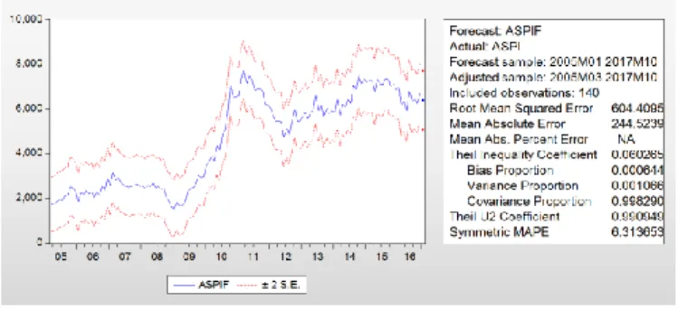
E. Forecasting
The forecasting value of October 2016 is 6367.313 with forecasting error 244.5239.
Figure 1: Plot of forecasting ASPI values
IV. CONCLUSION
The time series analysis is a useful methodology which comprises the tools for analyzing the time series data to identify the characteristics for making future adjudgements, especially for decision making in economic and finance.
This research focuses on building a model for Colombo stock market indices using this time series methodology. Monthly data of ASPI and SL20 for the period ranging from January 2005 to September 2016 and from June 2012 to August 2016 were used respectively. The most appropriate obtained for ASPI is the ARIMA (1, 1, 1).
REFERENCES
[1] Akuffo, B., & Ampaw, E. M. (2013). An Autoregressive Integrated Moving Average (ARIMA) Model For Ghana's Inflation(1985 - 2011). Mathematical Theory and Modeling, 3, 213 - 216. Retrieved 2016 [2] RM Kapila Tharanga Rathnayaka, DMKN Seneviratna, Wei Jianguo,
“Grey system based novel forecasting and portfolio mechanism on CSE”, Grey Systems: Theory and Application, 6(2), 126-142, 2016, Emerald Group Publishing Limited; http://dx.doi.org/10.1108/GS-02-2016-0004
[3] Ho, S. L., & XIE, M. (1998). THE USE OF ARIMA MODELS FOR RELIABILITY FORECASTING AND ANALYSIS. 23rd International Conference on Computers and Industrial Engineering (pp. 213 - 216). Great Britain: Elsevier Science Ltd.
[4] RM Kapila Tharanga Rathnayaka, DMKN Seneviratna, Wei Jianguo, “Grey system based novel approach for stock market forecasting”, Grey Systems: Theory and Application, 5(2), 178-193, 2015, Emerald Group Publishing Limited ; http://dx.doi.org/10.1108/GS-04-2015-0014 [5] Arumawadu, H.I., Rathnayaka, R.M.K.T. & Seneviratna, D.M.K.N.,
“New Proposed Mobile Telecommunication Customer Call Center Roster Scheduling Under the Graph Coloring Approach” , International Journal of Computer Applications Technology and Research, 5(4), pp.234–237, 2016, www.ijcat.com.
[6] Hasitha Indika Arumawadu, RM Kapila Tharanga Rathnayaka, SK Illangarathne, “K-Means Clustering For Segment Web Search Results”, International Journal of Engineering Works, 2(8), 79-83, 2015, kwpublisher.com.
[7] R.M. Kapila Tharanga Rathnayaka and D.M.K.N Seneviratne, “G M (1, 1) Analysis and Forecasting for Efficient Energy Production and Consumption”, International Journal of Business, Economics and Managment works, Kambohwell Publisher Enterprises, 1 (1), 6-11, 2014, www.kwpublisher.com
[8] Hasitha Indika Arumawadu, RM Kapila Tharanga Rathnayaka, SK Illangarathne, “Mining Profitability of Telecommunication Customers Using K-Means Clustering”, Journal of Data Analysis and Information Processing, 3(3), 63, 2015, DOI: 10.4236/jdaip.2015.3300.
[9] R.M. Kapila Tharanga Rathnayaka and D.M.K.N Seneviratne, “A Comparative Analysis of Stock Price Behaviors on the Colombo and Nigeria Stock Exchanges”, International Journal of Business, Economics and Managment works, Kambohwell Publisher Enterprises, 2 (2), 12-16, 2014, www.kwpublisher.com .
[10] Jayathileke, P. M. B., and Rathnayaka, R.M. K. T. “Testing the Link between Inflation and Economic Growth: Evidence from Asia”, Modern Economy,4, 87, 2013, www.scirp.org .
[11] R.M Kapila Tharanga Rathnayaka, D.M. Kumudu Nadeeshani Seneviratne and Zhong- jun Wang, “An Investigation of Statistical Behaviors of the Stock Market Fluctuations in the Colombo Stock Market: ARMA & PCA Approach”, Journal of Scientific Research & Reports 3(1): 130-138, 2013; Article no. JSRR, www.sciencedomain.org [12] R.M. Kapila Tharanga Rathnayaka and Zhong-jun Wang, “Enhanced Greedy Optimization Algorithm with Data Warehousing for Automated Nurse Scheduling System”, E-Health Telecommunication Systems and Networks ,1(4), 2012, www.SciRP.org/journal/etsn
[13] Khashei, M., & Bijari, M. (2011). A novel hybridization of artificial neural networks and ARIMA models for time series forecasting. Applied Soft Computing, 2664 - 2675.
[14] R.M. Kapila Tharanga Rathnayaka, D.M.K.N Seneviratne, Wei Jianguo and Hasitha Indika Arumawadu, “A Hybrid Statistical Approach for Stock Market Forecasting Based on Artificial Neural Network and ARIMA Time Series Models”, The 2nd International Conference on Behavioral, Economic and Socio-Cultural Computing (BESC’2015-IEEE), Nanjing, China, 2015. http://besc2015.njue.edu.cn
[15] R.M. Kapila Tharanga Rathnayaka, Wei Jianguo and D.M.K.N Seneviratne, “Geometric Brownian Motion with Ito lemma Approach to evaluate market fluctuations: A case study on Colombo Stock Exchange”, 2014 International Conference on Behavioral, Economic, and Socio-Cultural Computing (BESC’2014- IEEE), Shanghai, China, 2014. http://datamining.it.uts.edu.au/conferences/besc14
[16] R.M. Kapila Tharanga Rathnayaka, D.M.K.N. Seneviratna, Wei Jianguo and Hasitha Indika Arumawadu, “An unbiased GM(1,1)-based new hybrid approach for time series forecasting”, Grey Systems: Theory and Application, 6(3), 322-340, 2016, Emerald Group Publishing Limited; http://dx.doi.org/10.1108/GS-04-2016-0009.
[17] Konarasinghe, S. W., Abenayake, R. N., & HGunaratne, P. L. (2015). ARIMA Models on Forecasting Sri Lankan Share Market Returns. International Journal of Novel Research in Physics Chemistry & Mathematics, 6-12.
[18] D.M.K.N. Seneviratna and Mao Shuhua, “Forecasting the Twelve Month Treasury Bill Rates in Sri Lanka: Box Jenkins Approach ”, IOSR Journal of Economics and Finance (IOSR-JEF), 1(1), 42-47, 2013. [19] McGough, T., & Tsolacos, S. (1995). Forecasting commercial rental
values using ARIMA models. Journal of Property Valuation & Investment, 6-22.
[20] Morawakage, S. P., & Nimal, D. P. (2015). Equity Market Volatility Behavior in Sri Lankan Context. Kelaniya Journal of Management, 4(2). [21] Donglin Chen, Dissanayaka M. K. N. Seneviratna, “Using Feed Forward BPNN for Forecasting All Share Price Index”, Journal of Data Analysis and Information Processing, 2(1), 87-94, 2014.
[22] Samarakoon, L. P. (1996). STOCK MARKET RETURNS AND INFLATION:Sri Lankan Evidence. Sri Lankan Journal of Management, 1(4), 293-311.
[23] Samayawardena, D. N., Dharmarathne, H. A., & Tilakaratne, C. D. (November 2015). Volatility Models for World Stock Indices and Behavior of All Share Price Index. Proceedings of 8th International Research Conference,KDU, (pp. 175-182).
[24] Stevenson, S. (2007). A comparison of the forecasting ability of ARIMA models. Journal of Property Investment & Finance, 223-578.
[25] Tsay, R. S. (2005). Analysis of Financial Time Series (2nd ed.). United States of America: Wiley - Interscience.
[26] Wickremasinghe, G. (2011). The Sri Lankan stock market and the macroeconomy: an empirical investigation. Studies in Economics and Finance, 179 -195.
[27] Zhang, G. P. (2003). Time Series forecasting using a hybrid ARIMA and nural network model. Neurocomputing, 159-175. Retrieved November 10, 2016, from http://www.elsevier.com/locate/neucom Capital market information center. Retrieved 4th December 2016, from [28]
http://www.cmic.sec.gov.lk/wp-content/uploads/2012/10/08Market-Indices-Monthly2.xls
[29] User, S. (2016). Stock Market. Taxplusinvestment.com. Retrieved 6 December 2016, from http://taxplusinvestment.com/index.php/stock-market
[30] Colombo Stock Exchange (CSE) | Colombo Stock Watch. (2016). Colombostockwatch.com. Retrieved 6 December 2016, from http://colombostockwatch.com/cse/