Dissertation
submittedto the
Combined Faculty for the Natural Sciences and Mathematics of
Heidelberg University, Germany
for the degree ofDoctor of Natural Sciences
Put forward by
Dipl.-Math Anke Mareike Schmidtobreick born in Karlsruhe
Oral examination: October 27, 2017
Parallel Asynchronous Matrix Multiplication
for a
Distributed Pipelined Neural Network
Advisors:
Prof. Dr. Vincent Heuveline JProf. Dr. Holger Fr¨oning
Either I will find a way, or I will make one.
(Philip Sidney)
Abstract
Machine learning is an approach to devise algorithms that compute an output without a given rule set but based on a self-learning concept. This approach is of great importance for several fields of applications in science and industry where traditional programming methods are not sufficient. In neural networks, a popular subclass of machine learning algorithms, commonly previous experience is used to train the network and produce good outputs for newly introduced inputs. By increasing the size of the network more complex problems can be solved which again rely on a huge amount of training data. Increasing the complexity also leads to higher computational demand and storage requirements and to the need for parallelization.
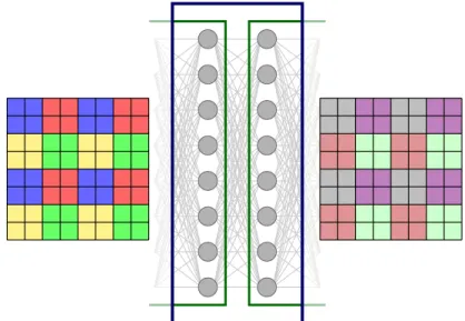
Several parallelization approaches of neural networks have already been considered. Most ap-proaches use special purpose hardware whilst other work focuses on using standard hardware. Often these approaches target the problem by parallelizing the training data. In this work a new parallelization method namedpoadSGD is proposed for the parallelization of fully-connected, large-scale feedforward networks on a compute cluster with standard hardware. poadSGD is based on the stochastic gradient descent algorithm. A block-wise distribution of the network’s layers to groups of processes and a pipelining scheme for batches of the training samples are used. The network is updated asynchronously without interrupting ongoing computations of subsequent batches. For this task a one-sided communication scheme is used. A main algorithmic part of the batch-wise pipelined version consists of matrix multiplications which occur for a special distributed setup, where each matrix is held by a different process group.
GASPI, a parallel programming model from the field of “Partitioned Global Address Spaces” (PGAS) models is introduced and compared to other models from this class. As it mainly relies on one-sided and asynchronous communication it is a perfect candidate for the asynchronous update task in the poadSGD algorithm. Therefore, the matrix multiplication is also implemented based GASPI. In order to efficiently handle upcoming synchronizations within the process groups and achieve a good workload distribution, a two-dimensional block-cyclic data distribution is applied for the matrices. Based on this distribution, the multiplication algorithm is computed by diagonally iterating over the sub blocks of the resulting matrix and computing the sub blocks in subgroups of the processes. The sub blocks are computed by sharing the workload between the process groups and communicating mostly in pairs or in subgroups. The communication in pairs is set up to be overlapped by other ongoing computations. The implementations provide a special challenge, since the asynchronous communication routines must be handled with care as to which processor is working at what point in time with which data in order to prevent an unintentional dual use of data.
The theoretical analysis shows the matrix multiplication to be superior to a naive implementation when the dimension of the sub blocks of the matrices exceeds 382. The performance achieved in the test runs did not withstand the expectations the theoretical analysis predicted. The algorithm is executed on up to 512 cores and for matrices up to a size of 131,072×131,072.
The implementation using the GASPI API was found not be straightforward but to provide a good potential for overlapping communication with computations whenever the data dependencies of an application allow for it. The matrix multiplication was successfully implemented and can be used within an implementation of the poadSGD method that is yet to come. The poadSGD method seems to be very promising, especially as nowadays, with the larger amount of data and the increased complexity of the applications, the approaches to parallelization of neural networks are increasingly of interest.
Zusammenfassung
Ein maschinelles Lernen Modell ist ein k¨unstliches System, das ohne einen vorgegebenen Regel-satz basierend auf vorherigen Erfahrungen eigenst¨andig lernt, zu unbekannten Eingaben passende L¨osungen zu produzieren. Dieser Ansatz ist f¨ur mehrere Einsatzgebiete von großer Bedeutung sowohl in der Wissenschaft als auch der Industrie, wenn traditionelle Programmiermethoden nicht ausreichen. In neuronalen Netzwerken, einer beliebten Unterklasse der maschinellen Lernalgorith-men, werden vorgegebene Trainingsdaten bestehend aus Ein- und Ausgabewerten verwendet, um das Netzwerk basierend auf der Differenz zwischen dem vorgegebenen Wert und dem Ausgabew-ert des Netzwerkes zu trainieren. Durch gr¨oßere Netze k¨onnen komplexere Probleme abgebildet werden, die wiederum auf das Vorhandensein einer großen Anzahl von Trainingsdaten angewiesen sind. Die Erh¨ohung der Komplexit¨at f¨uhrt so zu h¨oherem Rechenbedarf und h¨oheren Speicheran-forderungen, weshalb eine Parallelisierung des Trainings sinnvoll scheint.
Es wurden bereits mehrere Parallelisierungsans¨atze f¨ur neuronale Netze in Betracht gezogen. Viele Ans¨atze verwenden Spezialhardware, w¨ahrend sich andere Arbeiten auf die Verwendung von Stan-dardhardware konzentrieren.
In dieser Arbeit wird eine neue Parallelisierungsmethode namens poadSGD vorgestellt, welche sich an vollst¨andig verbundene, sehr große Feedforward-Netzwerke richtet, welche auf einem Rechen-cluster mit Standardhardware ausgef¨uhrt werden. PoadSGD basiert auf dem stochastischen Gra-dientenverfahren und verwendet eine blockweise Verteilung der Netzwerkschichten auf Gruppen von Prozessen, sowie ein Pipeline-Schema, das jeweils f¨ur eine Serie von Trainingsdaten ausgef¨uhrt wird. Das Netzwerk wird asynchron aktualisiert, ohne die noch laufenden Berechnungen der nach-folgenden Serien zu unterbrechen. Hierf¨ur wird ein einseitiges Kommunikationsschema verwendet. Ein wesentlicher Teil des Algorithmus sind Matrixmultiplikationen, wobei f¨ur einen Teil davon der Fall auftritt, dass die Matrizen auf jeweils unterschiedliche Prozessgruppen verteilt sind.
In dieser Arbeit wird daher GASPI, ein paralleles Programmiermodell aus dem Bereich der Parti-tioned Global Address Spaces(PGAS) Modelle, vorgestellt und mit anderen Modellen dieser Klasse verglichen. Da es haupts¨achlich auf einseitiger und asynchroner Kommunikation basiert, ist es ein perfekter Kandidat f¨ur die Umsetzung des asynchronen Updates im poadSGD-Algorithmus. Daher ist die Matrixmultiplikation auch auf der Basis von GASPI implementiert. Um eine gute Verteilung der Arbeitslast zu erreichen und m¨oglichst effizient mit der Synchronisation, die durch die zusam-menarbeitenden Prozessgruppen entsteht, umzugehen, wird f¨ur die Matrizen eine zweidimensionale blockzyklische Datenverteilung angewendet. Basierend auf dieser Verteilung wird der Algorithmus f¨ur die Matrix-Multiplikation durch eine diagonale Iteration ¨uber die Teilbl¨ocke der Ergebnismatrix und die Berechnung dieser Teilbl¨ocke in Untergruppen der Prozessgruppen umgesetzt. Die Rechen-last der Berechnung der Teilbl¨ocke wird zwischen den Gruppen aufgeteilt und die Kommunikation findet haupts¨achlich paarweise oder nur in Untergruppen statt. Die paarweise Kommunikation erfolgt so, dass sie von anderen laufenden Berechnungen ¨uberlappt wird. Die Implementierung des Algorithmus stellt eine besondere Herausforderung dar, da die asynchronen Kommunikationsrou-tinen mit Sorgfalt gehandhabt werden m¨ussen. Es muss zu jedem Zeitpunkt klar sein, welcher Prozessor mit welchen Daten arbeitet oder wohin versendet, um eine unbeabsichtigte doppelte Nutzung von Daten zu verhindern.
Die theoretische Analyse zeigt, dass die hier pr¨asentierte Matrixmultiplikation einer naiven Imple-mentierung ¨uberlegen ist, wenn die Dimension der Teilbl¨ocke der Matrizen gr¨oßer als 382 ist. Diese Erwartung hat die in den Testl¨aufen erzielte Performance nicht erf¨ullt. Der Algorithmus wurde auf bis zu 512 Kerne f¨ur Matrizen bis zu einer Gr¨oße von 131.072×131.072 ausgef¨uhrt. Die
Auch wenn die Performance nicht den Erwartung entsprach, so wurde die Matrixmultiplikation erfolgreich umgesetzt und kann f¨ur eine Implementierung der poadSGD-Methode verwendet wer-den. Der Ansatz der poadSGD-Methode ist sehr vielversprechend, zumal heutzutage mit den immer gr¨oßeren Datens¨atzen und der erh¨ohten Komplexit¨at der Anwendungen die Ans¨atze zur Parallelisierung von neuronalen Netzwerken zunehmend von Interesse sind.
Mathematical Contributions
The approach of machine learning is of great importance, both in science and in industry, when traditional algorithms are no longer sufficient.
In this work a parallelization method for large-scale feedforward neural networks is pre-sented. The method used for its training thereby relies on the stochastical gradient descent method and is combined with a block-wise distribution of the network layers to groups of processes, as well as a pipelining scheme for batches of the training samples and an asynchronous update of the network.
A particular challenge of the proposed method is a matrix multiplication for very large matrices with a special parallel distribution of the matrix elements. For this particular configuration, a parallel algorithm is developed based on asynchronous communication mechanisms, which have an impact on the algorithmic implementation. In addition, the algorithm is analyzed with regards to its communication complexity and its potential for exploitation of overlapping communication and computation enabled by the asynchronous communication. Through the development and implementation of the matrix multipli-cation for the parallelization of neural networks, experience in the use of asynchronous communication for basic, numerical methods is gained.
Acknowledgments
Finally, the end of my PhD time has come, it had its ups and downs. During this time I had the pleasure to get to know and appreciate three different universities: Karlsruhe Institute of Technology (KIT), the University of Oxford and finally for most of the time the oldest university of the country: Heidelberg University, Ruperto-Carola.
Therefore my thanks go out to different locations: first of all to Prof. Dr. Vincent Heuveline first at KIT and then at the Faculty of Mathematics and Computer Science at Heidelberg University for giving me this great opportunity for my PhD. Also, I am very grateful for his continuous support and guidance during my time as a PhD student. In addition, I am grateful to JProf. Dr. Holger Fr¨oning for his quick and eager agreement to support me as my second supervisor and thereby provide me with good advice. Fur-thermore, my thanks go to Prof. Endre S¨uli who welcomed me to the Numerical Analysis Group at the University of Oxford and made my research stay possible, it was a great experience.
Also thanks for all the encouragement and motivation boosts from all kinds of places: from the place opposite or next to mine (in all offices and trains), from neighboring offices, from family and friends, former and current colleagues, via e-mail or live – biggest thanks!
I would also like to acknowledge the “Karlsruhe House of Young Scientists (KHYS)” which funded my research stay at Oxford University and the support by the state of Baden-W¨urttemberg through bwHPC and the German Research Foundation (DFG) through grant INST 35/1134-1 FUGG in terms of the computational resource that was used in this work.
Contents
Chapter1 –Introduction 1
1.1 Contributions . . . 3
1.2 Structure . . . 4
Chapter2 –Neural Networks 5 2.1 Introduction to Machine Learning . . . 5
2.2 Fundamentals of Neural Networks . . . 7
2.2.1 Components and Basic Functionality . . . 8
2.2.2 Training a Neural Network . . . 11
2.2.3 Different Network Models . . . 15
2.2.4 Challenges, Optimization and Regularization . . . 18
2.3 Parallelizing Neural Networks . . . 21
2.3.1 Hardware Employed . . . 22
2.3.2 Types of Parallelization . . . 22
2.3.3 Review of Parallelization on CPUs . . . 23
2.4 New Parallel Method poadSGD . . . 25
2.4.1 Key Ideas of poadSGD . . . 26
2.4.2 The poadSGD Algorithm . . . 29
2.4.3 Distribution of Weight Matrix . . . 30
2.4.4 Outlook . . . 32
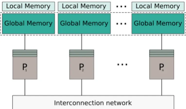
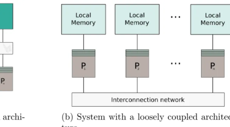
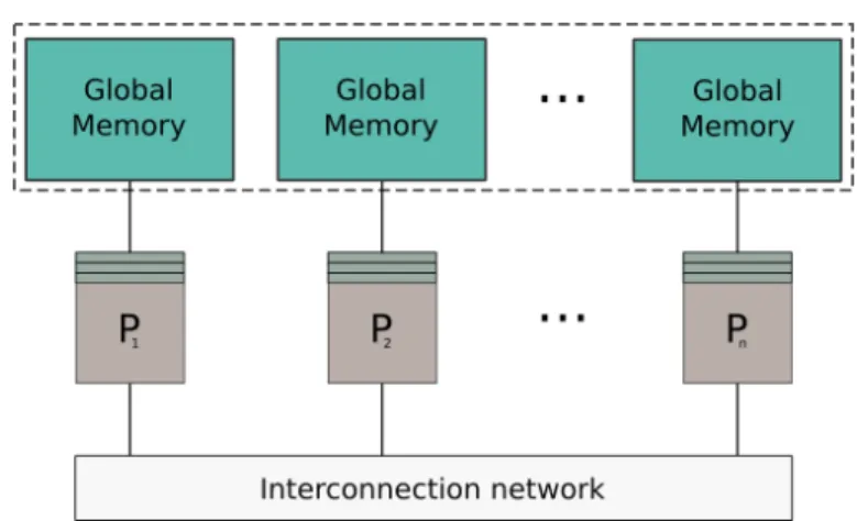
Chapter3 –Parallel Computing Models 35 3.1 Classifying The Parallel World . . . 35
3.1.1 Classification based on the Memory Architecture . . . 36
3.1.2 Classification based on Parallel Programming Models . . . 37
3.2 The PGAS Model . . . 39
3.2.1 Coarray Fortran (CAF) . . . 40
3.2.2 Unified Parallel C (UPC) . . . 42
3.2.3 Further PGAS-based languages . . . 44
Chapter4 –Global Address Space Programming Interface (GASPI) 47 4.1 GASPI’s Origin . . . 47
4.2 GASPI Specification and Functionalities . . . 48
4.2.1 Process and Memory Setup . . . 49
4.2.2 General Concepts of GASPI Functions . . . 51
4.2.3 Synchronization . . . 52
4.2.4 One-sided Communication . . . 52
4.2.5 Collectives . . . 56
4.2.6 Further GASPI Features . . . 57
4.2.7 Overlap of Communication and Computation . . . 58
4.3 Comparing Features: GASPI vs. CAF & UPC . . . 59
Chapter5 – Dense Matrix Multiplication in GASPI 65
5.1 Matrix Representation . . . 66
5.2 A Matrix Multiplication Algorithm with GASPI . . . 69
5.2.1 Related work . . . 69 5.2.2 Implementation . . . 71 5.2.3 Theoretical Analysis . . . 78 5.3 Performance Tests . . . 91 5.3.1 Test Setup . . . 91 5.3.2 Results . . . 97
Chapter6 – Conclusion and Outlook 103
References 117
Chapter
1
Introduction
In a field where adequate rules are too difficult to devise for a given problem, classical programming approaches are not sufficient and instead machine learning algorithms are applied. These algorithms follow the concept of learning to solve a problem based on previous experiences. They are then able to generalize and to produce solutions for inputs they have never seen before. Machine learning has become of great importance in science and industry. Amongst others, it is used to solve problems from the fields of medical ap-plications, image and voice processing, search engines and social networks [Sch14, Nie15]. A classical machine learning algorithm is the artificial neural network. Originally inspired by the human brain it is built up of several layers of neurons connected by synapses which transfer signals throughout the network and generate a solution when given a new input. Algorithms have been developed to optimize such a network by adapting the parameters of the network during a training phase based on previous training data. Increasing the size of these networks enables more complex problems to be solved. But this also leads to issues with the convergence of the training that need to be dealt with. Equally important is that the higher complexity also increases the computational demand and the storage requirements [PLWH03]. A solution to this is to parallelize these networks. However, to efficiently accomplish this task, several factors are of great importance: which hardware is selected, which parallel programming model suits the problem best and finally how ex-actly the algorithm is parallelized such that it scales well for differently sized networks and generates no unnecessary overhead.
For the training phase different parallelization approaches of neural networks have al-ready been considered [RS97]. Most approaches use special purpose hardware such as GPUs [DCM+12] or specialized neuromorphic computers [FFA92, SBG+10]. But, as this
special hardware is not always available in all research labs and universities, other works focus on using standard hardware. The parallelization techniques used include the run-ning of several instances of the network in parallel [PLWH03]. Either these instances are started with the same initial state or different ones. Furthermore, they can all be trained with the same training input or with different parts of the data. After the separate train-ing the results are reconciled. Other techniques parallelize the traintrain-ing inputs for a strain-ingle network, pipeline the training samples or partition the network topology itself amongst several processes [NS92]. For parallelization on CPUs, MPI is often used for the commu-nication between the processes, for example in [DMN08]. Furthermore, the update of the networks’ parameters often occurs in a synchronized way by a central instance [DCM+12],
limiting the efficiency.
This thesis devises an efficiently parallelized algorithm namedpoadSGD for the training of a neural network, when using a compute cluster with standard hardware. The focus is on the question whether an improvement of the performance can be achieved by using differ-ent communication schemes as provided by the partitioned global address space (PGAS) programming model. One such model is GASPI [Con13] which relies only on one-sided and asynchronous communication patterns. This leverages the idea of devising a batch-wise variant of the stochastic gradient descent method with a pipelining scheme where GASPI allows for an asynchronous update. The poadSGD algorithm maps the network layer-wise to different groups of processes, together achieving a pipeline which processes several batches of training samples directly after another. The updates are computed by averaging the updates of a batch and applying the result directly to the network. Updates are thereby sent asynchronously without interrupting ongoing computations of subsequent batches. The main algorithmic part of the pipelined version is the matrix multiplication which occurs for a special distributed setup, namely each matrix being held by a different process group. All in all, the main research question thereby is how to efficiently imple-ment a scalable version of this matrix multiplication where both matrices are distributed amongst different process groups and when employing the asynchronous and one-sided communication scheme of GASPI.
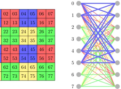
In order to efficiently handle upcoming synchronizations within the process groups and achieve a good workload distribution, a two-dimensional block-cyclic data distribution is applied for the matrices. Thereby, a matrix is divided into sub blocks and these are mapped to individual processes by means of a process grid containing the processes associated with the matrix. A structure is defined which simplifies the determination of the exact location of each matrix element. As a result, the computation of each sub block of the matrix resulting from the matrix multiplication only depends on the processes in a row of the process grid of the first matrix and the processes in a column of the process grid of the second matrix. Therefore, the first computational scheme is to diagonally iterate over these sub blocks and compute the sub blocks which allows for a maximum number of blocks to be computed in parallel. At the heart of the method is then the overlap algorithm. Here, processes first work in pairs where one process is from each of the matrix groups. The algorithm is implemented with a focus on achieving an overlap of the communication between these pairs of processes with ongoing computations. Furthermore, based on the setup of the process grid, the algorithm makes use of the process grid topology to apply reduction operations on sub-groups of the process grid.
The result is an implementation of the matrix multiplication for dense matrices relying on GASPI’s features with a special focus on its asynchronous communication scheme. The approach is analyzed theoretically with regard to its capability for overlap for its two main parts: thediagonal iteration over the blocks of the result matrix and theoverlap algorithm which is the main part of the computation of these blocks. The diagonal iteration proves to always be superior to a naive implementation and the overlap algorithm is shown to improve performance when the dimension of the blocks exceeds 382. In addition, the strong and weak scalability on a high performance cluster is evaluated. As a first step, for each combination of possible number of processes and size of the matrices, the block size with the best performance is chosen for further tests. For these parameter combinations the matrix multiplication is then run on up to 512 cores and for matrices up to a size of 131,072×131,072 (≈17.2 billion elements). The performance achieved in the test runs did not withstand the expectations the theoretical analysis had promised. The speedup and efficiency highly depend on the matrix size used. They were determined with respect
1.1. Contributions 3
to the results achieved on the smallest process grids with 4 processes each, such that the ideal speedup is 64 for the largest process grid. The efficiency is about 0.2 or better for matrices smaller than 1024×1024 but for larger matrices it drops drastically when increasing the number of processes.
The implementation using the GASPI API were found to be tedious as GASPI does not provide a black-box with easy-to-use communication calls, but provides a clearly structured interface that leaves many details to the user such as the management of the position of global data (in terms of offsets) and handling of buffers. Also correctly implementing with GASPI proves to be a challenge as it requires a deep understanding of the underlying functionality. However, the matrix multiplication was successfully implemented for the special setup of matrices distributed across multiple process groups and based on GASPI, although the results achieved by the test runs were below expectations. As a follow-up step a performance analysis tool could be employed in order to detect which points of the current algorithm could be optimized. Of further interest would be a complete implementation of the poadSGD method based on an asynchronous framework such as GASPI or to adapt an existing software framework for neural networks for this task.
1.1
Contributions
To provide a better overview, the author’s contributions are listed in this section.
An introduction to machine learning and neural networks is given, also providing an overview of parallelization techniques.
The author presents a new pipelined method poadSGD for the parallel implementa-tion of large-scale fully-connected feedforward networks which is based on one-sided and asynchronous communication schemes.
As in literature parallel models are described differently, this work presents an overview of the different categorizations. This enables the user to understand the context of PGAS models and to better understand the shift from comparing com-puter architectures to comparing memory models of programming languages. An introduction to GASPI is presented, providing an understanding of its one-sided
and asynchronous communication model and how it affects the development of an algorithm. Possibilities how GASPI’s communication routines are used and how they can be employed to overlap communication with computation are demonstrated by small examples.
A description of the matrix multiplication algorithm based on a PGAS-model with one-sided and asynchronous communication, written in C and GASPI, is presented. Divided into two main sub algorithms, an analysis of the combined arithmetical and communication complexity is given. Thereby the focus is on determining if or when overlap occurs and how it may increase the overall performance of the application. Moreover helpful approaches for future numerical implementations are given: ideas
how to realize algorithmic steps and for the theoretical analysis of such algorithms, how data usage and active processors in each algorithmic step may be represented and that close attention has to be paid to the data dependencies.
Possible extensions and improvements are put forward, both for the author’s imple-mentations to improve the current implementation and for the GASPI standard to lower the entry threshold for new users.
1.2
Structure
The structure of this thesis is divided into six parts.
Chapter I - Introduction The first chapter gives a short motivation of this thesis, ad-dressing the class of machine learning algorithms and focusing on artificial neural networks and their significance in today’s world. Furthermore, the need for paral-lelization of the training methods of these models is described.
Chapter II - Neural Networks A general introduction into machine learning is given based on the description of a simple feedforward network (FNN) and a presentation of a common learning method, the backpropagation. The task of parallelizing large-scale FNNs is put forward and different parallelization techniques are discussed. Finally a new parallelization approach is proposed: the poadSGD method. It is de-scribed and its key requirements regarding the asynchronous communication scheme and the main algorithmic part, the matrix multiplication for a special distributed case are explained.
Chapter III - Parallel Computing Models In this chapter different parallel comput-ing models are introduced, leadcomput-ing to the definition of the PGAS model and endcomput-ing with a brief presentation of the two main PGAS languages and a short overview of further PGAS languages.
Chapter IV - GASPI At the start of this chapter, the parallel programming model GASPI is introduced. A brief outlook on its history is given and then GASPI’s main features are described. The introduction is illustrated by small, numerical examples. Finally GASPI’s main characteristics are compared to those of two other PGAS languages, UPC and CAF.
Chapter V - Dense Matrix Multiplication in GASPI This chapter first introduces the data distribution and its implementational concept that is key to the implemen-tation of the algorithms as it also is the basis for the later work distribution. Here-inafter the implementation of a matrix multiplication is presented which applies to the special case of the matrices residing on different process groups. It is followed by a theoretical analysis of its algorithmic parts. Finally, the results of different runs on a high performance cluster and the achieved scalability are discussed.
Chapter VI - Conclusion and Outlook The last chapter starts with an overview of the work accomplished in this thesis. The results are discussed and additionally, an overview of possible extensions and improvements is given. Finally, the work is concluded by giving an outlook on future development in parallel programming and the future significance of machine learning.
Chapter
2
Machine Learning and Neural
Networks
After their first showdown in the 60s/70s, with the rediscovery of the backpropagation algorithm and the development of further network topologies, neural networks experienced a revival in science and industry.
This chapter gives a general introduction to machine learning, focusing hereby on the sub-class of artificial neural networks. First, a simple version of a feedforward network and its learning method is introduced. The section thereafter presents variations to this network model and describes different optimization opportunities. This information is provided in order to give a more complete overview of this field but is not required in order to understand the whole of this thesis. Then, turning back to the basic feedforward network, the parallelization possibilities of neural networks are explained and an emphasis is put on the parallelization realized on generic compute clusters. Finally, a new parallelization approach is presented in order to achieve a pipelined, distributed version of a feed-forward neural network. The approach combines known with new parallelization techniques and leads to both a rethinking of the parallel paradigms used, as well as points out the need to further discuss a large-scale matrix multiplication.
The first section of this chapter is based on knowledge gained from various sources: the online book of Michael A. Nielsen [Nie15], a very detailed review paper in preprint form by J¨urgen Schmidhuber [Sch14], the Coursera online course “Machine Learning” by Associate Professor Andrew Ng from Stanford University [Ng16] and a book on machine learning from Kevin P. Murphy [Mur12].
2.1
Introduction to Machine Learning
Learning to program most often one starts out with classic programming languages. A problem is given and an algorithm is devised to solve this problem. A prominent example from first year’s programming class is to write code that imitates a calculator. Enter some numbers and operations and get the according results as an output. But a problem setup may also be much more complex and therefore require skilled and challenging programming code for solving it.
However, for the implementation of the calculator example, the rules for the computational steps are well known and taught at every school. But for other problems there may not be
such a simple recipe for solving, meaning they may not have a predefined set of explicit rules for the solution steps. An example are the tomography screens of a patient who has a brain tumor. Based on these pictures, writing an application that determines whether the tumor is malignant or benign is no straight-forward task but overly complex and it requires medical experience.
Here a different programming approach may step into place: machine learning. Arthur Samuel coined this term in 1959 and denotes machine learning1 as the . . .
“. . . field of study that gives computers the ability to learn without being ex-plicitly programmed.”
This means learning how to solve a given problem without specifying any rules. Of course this does not mean that machine learning is a panacea with no effort or computational cost involved. In machine learning the algorithm is often learned based on previous experience. Input and output pairs are provided to the machine learning algorithm which then needs to decide on its own how to get from input to output.
Tom Mitchell gives a more formal definition [Mit97]:
“A computer program is said to learn from experience E with respect to some class of tasks T and performance measure P if its performance at tasks in T, as measured by P, improves with experience E.”
So a doctor may provide several pictures of brain tumors and label each picture with the additional information whether it is malignant or benign. These labelled pictures are the previous experience E. The task T of the program would be to develop an algorithm which produces the risk classification for the current picture as well as newly added ones. Mea-suring the performance P would be equal to counting the number of correctly classified pictures. The derived algorithm would be acknowledged as “learning”, if the number of correctly classified pictures increases.
Further applications arise from a wide range of topics, such as ([Sch14]): image recognition and classification,
image segmentation, object detection, speech recognition, sequence recognition or propositional logic.
Concrete examples include the recognition of fingerprints, the detection of specific persons or faces in photographs or surveillance videos and the detection of fraud payments by credit card. Medical applications, such as the discovery of a tumor or its classification, can benefit from machine learning, too. Today, machine learning is already employed by miscellaneous companies, such as Google (search engine), Microsoft or Facebook (social network analysis) [Nie15].
1
Note that this quote is cited multiple times throughout literature but the author could not track down the original source. It is sometimes referenced as a quotation from Samuel’s paper on checkers [Sam59] (which is not true) and also cited as a quotation from an article in the “The New Yorker and Office Management” from 1959 [JEG16] to which the author had no access.
2.2. Fundamentals of Neural Networks 7
Classifications of Machine Learning Algorithms
The machine learning model is rather a generic concept. Algorithms following this model can be classified into three main categories: supervised, unsupervised and reinforcement learning [Mur12]. Depending on the literature the algorithms are categorized into more differentiated subcategories including semi-supervised and active learning.
Forsupervised algorithms2 the previous experience E from Mitchell’s model consists of a given data set together with correct outputs which the algorithm shall be able to reproduce most accurately. This type of algorithm can be applied to two different types of problems: regression problems for which the predicted result is continuous orclassification problems where the output is discretely valued. An example for the first problem type could be the prediction of rental costs based on rentals of the previous years, whilst the formerly mentioned tumor classification turns out to be a classification problem.
Unsupervised algorithms3 on the other hand only provide data input but no correct output or concrete goals. The rather general purpose often is to find some kind of structure within the input data. Again two different types of problems can be identified: clustering and non-clustering problems. As the name indicates, the clustering problem strives to find some kind of clustering of the data based on some relationships within the data. The non-clustering problem on the other hand looks for some other kind of structure. An example for the clustering problem is the grouping of news entries from different websites based on common topics as it is used by search engines. A different example may be the grouping of people in an election into groups of voters, undecided voters and non-voters based on a social analysis of their profile in a social network for further campaigns. A prominent non-clustering problem is the cocktail party problem which opts for filtering single voices from different sound recordings at a party.
For the third type of machine learning, reinforcement learning, no samples are given. Instead, learning occurs by means of encouragement, so it is based on rewards or punish-ment signals given by its environpunish-ment throughout the learning process. This is what most closely resembles the way humans learn, for example when learning how to walk.
This thesis concentrates on the category of supervised learning.
2.2
Fundamentals of Neural Networks
There are several approaches to solving supervised machine learning problems. They range from learning based on a decision tree over applying support vector machines (SVM) or genetic algorithms to artificial neural networks and deep learning. In this section some concepts of machine learning are introduced based on the example of anartificial neural network (ANN), often also simply referred to as neural network, with a training algorithm used quite often, the backpropagation. The backpropagation algorithm was originally introduced in the 1970s, but its importance wasn’t fully appreciated until a famous paper on that topic was published by David Rumelhart, Geoffrey Hinton, and Ronald Williams in 1986 (republished later as [RHW88]).
Biological Background
The original inspiration of neural networks was the information processing of the human brain. Why so? In comparison, computers already are quite large: they have up to and
2
Also known as “predictive” algorithms [Mur12]. 3
probably by today more than 109 transistors with a switching time of 10−9seconds [Kri07].
However, a human brain has about 1011 neurons with a switching time of only 10−3
seconds. Furthermore, the brain with its rather simple layout can work massively parallel, can reorganize itself (some parts are able to take over tasks of other brain parts) and are fault tolerant against internal or external errors (up to a certain degree). Additionally, the brain is able to learn, either from training samples or by means of encouragement. A computer today is able to compute in parallel and there are certain means as to fault tolerance. But both are not as powerful as the human brain’s performance and telling one part of a computer to cope for other failing parts is seemingly impossible. Picking up on these qualities, the artificial neural network, commonly known as neural network, was derived.
First, we take a step back and explore the “architecture” of a human brain in a simplified way and then we follow up on the artificial neural network. The information on the biological background was taken from [Kri07] and simplified a bit, focusing on the main characteristics of the brain’s functionality. The major players of the human brain are the neurons. A neuron may be viewed as a switch with an information input and an information output. Even a fly already has about 105 neurons and humans with their 1011
neurons are again topped by elephants and some whale species who have twice as many. The neurons transfer information to other neurons via synapses. These can be electrical or chemical synapses. A chemical synapse is interrupted by a gap, the so-called synaptic cleft. In short, the incoming electrical signal is transformed into a chemical signal, some chemical processes occur in the cleft and the output is converted into an electrical signal again. The electrical signal then arrives at the neuron. The cell nucleus accumulates all the signals it receives from different synapses (from other neurons) into a single pulse. When the accumulated signal exceeds a certain threshold potential, an electrical pulse is sent on to other neurons.
2.2.1 Components and Basic Functionality of a Neural Network
The artificial neural network started out as a caricature of biology. The neurons, synapses and their functionality are the basic components of a neural network. Note, that there is not a single “neural network”. There is a common basis of the structure and functionality and from there different neural networks have evolved. Next, a basic setup of a neural network is introduced.
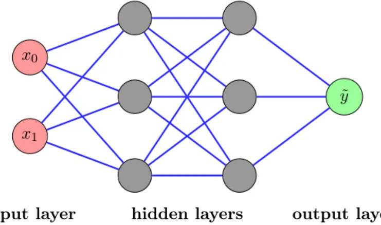
Figure 2.1 shows an exemplary graphical representation of an artificial neural network. In the figure, the neurons are depicted as circles and are arranged in several vertical layers. Here, a distinction is made between the neurons in the first (most left) input layer, the output layer (most right) and the so-called hidden layers in-between. The connections between them correspond to the synapses. These are tagged with a certain weight value to account for the variability of the chemical processes in the synaptic cleft.
The basic functionality of a neural network can be viewed as the analysis of a given problem on the basis of several differently weighted decision levels. Consider the problem of identifying the fruit shown in a given picture (or set of pictures). The layers could represent different decision levels to this question. The first layer would take the picture in form of its pixels and hand this information on to the next hidden layer. This layer could, for example, detect the shape of the fruit. Based on the shape the next layer could decide on the main color within this shape. Then, another layer could categorize the texture of the shape and so on. The output of the last layer would be a number representing a certain kind of fruit.
2.2. Fundamentals of Neural Networks 9
x1
x0
input layer hidden layers
˜ y
output layer
Figure 2.1: Depiction of a small neural network with two hidden layers.
Now how does this neural network work? In the 1950s/60s Frank Rosenblatt defined the network as above with perceptrons (artificial neurons) which take a binary input and output [Nie15]. Each perceptron (in one of the hidden or output layers) receives several input values via the incoming synapses which are additionally each provided with a weight. The binary output of a perceptron then depends on whether the sum of all weighted inputs exceeds a perceptron-specific threshold or not.
x1
x0 w b
0
w1
Figure 2.2: Single perceptron of a hidden layer within a neural network with weighted input synapses w0 and w1 and biasb.
The output of the perceptron in Figure 2.2 is then computed as
output =
(
1, ifw0x0+w1x1 ≥threshold
0, ifw0x0+w1x1 <threshold
or rewriting this equation as
output = ( 1, if P jwjxj+b≥0 0, if P jwjxj+b <0,
where thebias b acts as the negative threshold. The perceptron in this picture makes its decision by weighing up the results of the former layer, in this case the input layer. However with these binary-valued perceptrons making small adjustments to some weights may result in large changes to the output. To avoid that, the sigmoid neuron may be used: its input and output values are real-valued and range from 0 to 1 and the function
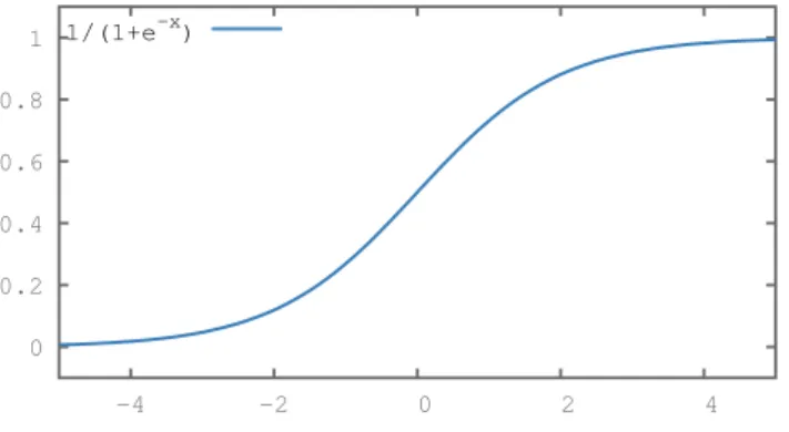
determining the output is chosen such that small changes to the weights only cause small changes to the output. The corresponding function is referred to as sigmoid as it is often shaped like an “S” (see Figure 2.3). More generally, the sigmoid neuron is simply called
0 0.2 0.4 0.6 0.8 1 -4 -2 0 2 4 1/(1+e-x)
Figure 2.3: Sigmoid function often used in a neural network (see Equation (2.1)).
“the” neuron, not placing any restrictions to the output function which is then called activation function a(). Its task is more generally the limitation of the amplitude of the output of the neuron. Still, most commonly a sigmoid function is used, for example
σ(z) = 1
1 + e−z, (2.1)
where zis the sum of the weighted inputs.
Formal Definition of a Neural Network
An (artificial) neural network is a network consisting of multiple layers of neurons which are connected by weighted synapses and typically modelled as a graph. More formally the topology of the network is a triple (N, W, B) of neurons, weighted synapses and biases. The set of neurons is denoted layer-wise as a vector:
N :={nl |njl variable denotingj-th neuron inl-th layer, l∈[0, L]}. (2.2) Similarly, the set of weighted synapses is a set of matrices where each matrix contains the weights on the synapses between the (l−1)-th and thel-th layer:
W :={Wl |wijl := (Wl)ij is weight between nlj−1 and n l
i, l∈[1, L]}. (2.3)
Finally, each neuron is assigned a bias which is represented accordingly as a vector in each layer, too:
B :={bl |blj is bias of neuron nlj, l∈[1, L]}. (2.4) The first column of neurons with l = 0 is the input layer with no incoming connections or biases. The last column l =L is the output layer with no outgoing connections. For now it is assumed that neurons of neighboring layers are fully connected and the graph is
2.2. Fundamentals of Neural Networks 11 nlj−1 blj−1 nli bli wl ij
Figure 2.4: Two neurons from subsequent layers with weighted synapses and the corre-sponding biases.
acyclic, so without loops and synapses do not skip layers. Whilst the weights and biases are real values,nlj is only a variable used to clarify which node is meant. The indexing of these components is illustrated in Figure 2.4.
Each layer l ∈ [1, L] corresponds to a function f(l) which for the neurons of each layer
accumulates the weighted inputs and computes the activation functiona for the inputx:
xl:=f(l)(x) =a(zl), where (2.5)
zl=Wlxl−1+bl. (2.6)
Here,xl−1 denotes the input vector to the synapses leading to layer l and is equal to the output of the former layer. The dimension changes accordingly to the number of neurons in each layer. The input vector x0 is usually simply denoted as vector x ∈ Rm (or in a
normalized fashionx∈[0,1]m) withmbeing the number of input elements for one sample.
The same applies to the output which is displayed as y ∈ [0,1]m with m specifying the
number of output components. The auxiliary vectorz is also named the weighted input. Note that the activation function is applied element-wise.
The neural network then is a functionf :x7→y˜consisting of multiple chained functions
f(x) =f(L)(f(L−1)(...f(1)(x)...)) = ˜y (2.7) and dependent on the weightsW, the biasesB and the activation functionais applied4.
Note that a network where the output of one layer corresponds to the input of the next is called afeedforward neural network. This particularly requires the graph to be acyclic.
2.2.2 Training a Neural Network
The basic concept of the neural network’s supervised learning (or the user training it) is based on two steps: First the output of the network f(x) = ˜y is computed for a given training sample {(x, y)}. Based on a cost function that uses the difference between the network’s output ˜yand the known solutionyan optimization of the neural network is then computed. Thereby the parameters of the network are adapted, namely the weights W (see Equation (2.3)) and the biasesB (see Equation (2.4)). This is carried out successively for each training sample given.
However, not all available training samples are used for the training of the network. In-stead, the set of training data is subdivided into two (sometimes three) data sets: a training
4
A mathematically better notation would bef(W, B, a, x) andf(l)(Wl, bl, a, x). However, the additional variables are omitted for a better readability.
set, a test set and sometimes also a validation set. The largest one, often two-third of the whole data set, is utilized for the training of the network. It is denoted as
(X, Y) ={(xj, yj) |(xj, yj) is a pair of the training set withj= 0, . . . , n−1, (2.8)
xj is the input vector, yj the desired output}.
In case an iterative approach is used, i. e., the training algorithm may iterate several times over this training set. The validation set may then be applied to decide whether or not to continue training. Note, that the validation set is only applied after a supposedly successful training. Finally, to evaluate the performance of the trained network, the test set is used. The performance metric is often determined as the proportion of samples of the test set for which answers are given correctly. With the test set one can see how the model reacts to data it has not seen before.
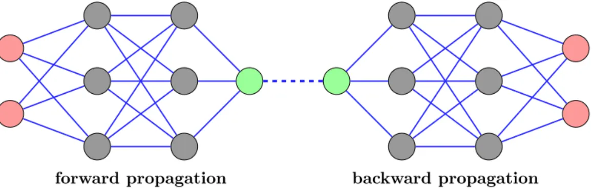
As mentioned above, the outputs computed by the neural network are needed in order to set up the cost function. This is done by propagating the input information from each sample xj of the training set through the network to get ˜yj. The formula for thisforward
propagation already was given in Equation (2.7) with the details noted in Equations (2.5) and (2.6).
In order to optimize the network, the backward propagation is employed. It was first defined by Rumelhart, Hinton and Williams in 1988 [RHW88]. They denoted it to be a procedure that . . .
“. . . repeatedly adjusts the weights of the connections in the network so as to minimize the measure of the difference between the actual output vector of the net and the desired input vector.” [RHW88]
The measure of difference mentioned by Rumelhart et al. is what in this work is called a cost function and is used to determine when a network has improved. The cost function used in this work is the mean squared error of the outputs. It is given in Equation (2.9).
C(W, B,(X, Y)) = 1 2n
X
xj∈X
kyj −f(xj)k2 (2.9)
This cost function is non-negative, quadratic and convex, improving the probability of finding a global minimum. Optimizing the neural network then corresponds to minimizing the cost function.
As a means of minimizing the cost function, the gradient descent (GD) method can be applied. In order to minimize a functiong(v) with parametersv= (v1, v2) the gradient of
the function ∇g= ∂g ∂v1 , ∂g ∂v2
is computed. The gradient then determines “the direction to go” to find the minimum. The GD law of motion [Nie15] then follows as:
∆v=−η∇g, (2.10)
2.2. Fundamentals of Neural Networks 13
Applying this law to the cost function (2.9) it yields the following update rules for the weights and biases:
wl,newij =wl,oldij −η ∇C
∇wijl , (2.11)
bl,newi =bl,oldi −η∇C
∇bli. (2.12)
The gradient of C (2.9) however, can also be seen as an averaged gradient of the sub-functions Cx = 12ky−f(x)k2. These subfunctions can be computed with the help of the
errorδjl in the j-th neuron of the l-th layer which is defined as follows: δjl := ∂Cx
∂zjl . (2.13)
The errorδjl accounts for a change of the weighted inputzjl in layerland therefore also for changes in the weights and biases. Applying the chain rule to Equation (2.13) the error for the last layer Lcan be computed as
δjL= ∂Cx ∂f(L)(x) j a0(zLj) = ∂Cx ∂y˜j a0(zLj). (2.14) This can also be written in vectorized form as
δL=DL∇xLC, (2.15)
where DL is diagonal matrix containing the entries a0(zL
i ) and ∇LxC the gradient vector
of C in layerL with respect to the samplex:
DL= diag(a0(zL)) = a0(zL 0) 0 . .. 0 a0(zL m) , ∇xC= ∂Cx ∂f(L)(x) 0 .. . ∂Cx ∂f(L)(x) m .
This error is then propagated backwards through the neural net, similarly to the forward propagation, yielding δl for l = L−1, . . . ,1 as presented in vectorized form in Equa-tion (2.16).
δl=(Wl+1)Tδl+1
a0(zl), l=L−1, . . . ,1 (2.16) Here,is the Hadamard product which computes the product of two vectors element-wise. The propagated errorδl can then be related to the gradients of Cx as follows:
∂Cx ∂bl =δ l, (2.17) ∂Cx ∂Wl =f (l−1) (x)δl. (2.18)
Based on these equations the new weights and biases of the neural network can be com-puted. All in all, Algorithm 1 describes one learning step of the neural network based on the GD method.
It is known, that GD does not always perform well. For example, methods also making use of the second derivative converge a lot faster. However, only using the first derivative makes computation simpler and can be implemented in an easier way [RHW88]. More details about the issues of GD are explained in Section 2.2.4.
// INPUT: Neural network (N, W, B) and training set (X, Y). // Initialization of network
1 setup network topology 2 initialize weights and biases
// Iterate over training set
3 for(x, y)j ∈(X, Y) do
// Feedforward of input
4 forl= 1,2, . . . , L do
5 compute the weighted inputzl as in Equation (2.6); 6 compute the output of this layerxl as in Equation (2.5);
7 end
// Backward propagation
8 compute the error δL in the neurons of layer Las in Equation (2.14); 9 update weightsWL and biasesbL as in Equation (2.11) and (2.12) ; 10 forl=L−1, . . . ,1 do
11 compute errorδl in the neurons of layerl as in Equation (2.16); 12 update weightsWl and biasesbl as in Equation (2.11) and (2.12) ;
13 end
14 end
Algorithm 1: Application of forward and backward propagation to a training set based on gradient descent.
In the setup of Algorithm 1, the network is trained with the same data (possibly in the same order) over and over again. Unfortunately, the backpropagation algorithm cannot be shown to converge [Hay09]. Therefore, some kind of stopping criterion is required to determine when the training is assumed to suffice. The computation of the gradient for the whole training set may take quite long [Nie15]. A variation of GD, the stochastic gradient descent (SGD) method therefore follows a different path to speed up the computation. The idea is to randomly divide the training set into smaller subsets and then train with each suchmini-batch one after the other. After having trained the network with each mini-batch, the validation set is applied and the percentage of correct answers determined. This validation step avoids overfitting. If the result is not good enough, another such epoch is started. Different mini-batches are randomly created and again trained one by one. Algorithm 2 shows the stochastic GD method. The size of the mini-batches s and the number of epochs E are freely selectable. If the sizes is chosen to be one, the method is called on-line learning.
2.2. Fundamentals of Neural Networks 15
// INPUT: Neural network (N, W, B) and training set (X, Y). // epoch
1 for e= 1, . . . , E do
2 randomly shuffle training data;
3 create mini-batches of size s: (X, Y)m={(xi, yi)∈(X, Y)|i=ms, . . . , ms+s};
// training of network on mini-batches
4 for m= 1, ..., M do
5 apply forward and backward propagation as in Algorithm 1 for neural network (N,W,B) and training set (X, Y)m;
6 end
// evaluate neural network
7 evaluate neural network with validation data; 8 if percentage of correct results high enough then
9 stop;
10 end
11 end
Algorithm 2:Stochastic gradient descent (SGD).
2.2.3 Characterizing Different Neural Network Models
In Section 2.2.1 a certain model of a neural network was introduced. But not all networks use the same topology or work the same way. In general, artificial neural networks can be characterized by three different properties [Lip88]:
network topology node characteristics training rules.
The first aspect refers to the number and type of layers of the neural network and to the connectivity structure in the neural net’s graph. Also, for some networks the topology may not be fixed but dynamically adaptable. The node characteristics are represented by the internal threshold (the bias) and the way a node processes its given inputs, including the non-linearity (the activation function) that is applied. Additionally, the node charac-teristics include the type of neuron activation, representing the moment when a neuron is activated. This can be done synchronously for all neurons of a network at once or asyn-chronously following the topological order or in a random order [Kri07]. The last aspect is the training rules. This is a broad field, ranging from choosing of the training set, ini-tializing the network’s parameters, choosing the loss function, determining how and when the network is updated down to deciding about the stopping criterion for the training. Some network models not only assume a certain topology but may also fix the activation function or the training algorithm to be used. This work focuses on the usage of feedfor-ward neural networks, like those encountered in Section 2.2.1. Beyond that, this section gives a short overview on the characteristics of different network models, as well as further activation functions and training algorithms for the interested reader. This overview is not necessarily required in order to understand the rest of this work but completes the basic overview of this topic. For more information on models and types of neural networks,
the author refers to a very detailed review paper from J¨urgen Schmidhuber [Sch14], cur-rently published as a preprint at this point. It contains a very detailed overview on the evolvement of neural networks up till 2014.
Models of Neural Networks
In Section 2.2.1, thefeedforward neural network (FNN) was introduced. It is a multi-layer network with synapses only pointing in the direction of the subsequent layer. Thereby the output of one layer is always the input to the subsequent layer, no information is ever fed back. In other words, the corresponding directed network graph is acyclic. The network always consists of an input layer, a number of hidden layers and an output layer. By increasing the number of hidden layers, the network may extract higher-order statistics from its input [Hay09]. The connectivity structure between layers and neurons depends on the network’s topology. A network is called fully connected when all neurons in a layer are connected to all neurons in the subsequent layer, otherwise it is called partially connected. At times, an FNN may also include shortcut connections: In this case a neuron is connected not only to the subsequent layer but also to another one closer to the output layer.
A special type of FNN is the convolutional neural network (CNN). In addition to the fully connected layers known from the FNN, it contains special layers such as convolutional layers (from which the name is derived) together with feature maps or subsampling lay-ers [BRSS15]. The convolutional layer extracts local features from its given input. This locality is implemented by connecting the neurons inside such a layer only to a few neu-rons of the previous layer which form a so-called local receptive field. Neuneu-rons which are part of feature maps share their weights, which leads to an invariance to shifts or certain transformations of the input data. This also reduces the number of parameters needed in the network. Pooling or subsampling layers perform a kind of non-linear down-sampling, thereby reducing the transferred data. The most common one is the max pooling. Com-binations of convolutional and pooling layers are also referred to as MPCNN networks. In general, a convolutional network is well suited for pattern classification and therefore often applied for image or video processing and operations involving the natural language. Some popular CNNs include the “LeNet”, the “AlexNet” and the LSTM network [Nie15].
Another network type is therecurrent neural network (RNN). The main difference between an RNN and an FNN is the removal of the feedforward restriction. In an RNN the synapses may also point backwards to a previous layer or back to a neuron itself. In other words, the corresponding directed network graph allows for backward connections and therefore cycles. Otherwise it is a static multilayer perceptron network [Hay09].
How does this affect the behavior of the network? Interpreting this in the biological sense, the neuron fires only for a limited time span [Nie15]. Firing backwards therefore does not affect other neurons instantaneously but in a different time step, avoiding dependencies. So whilst a CNN performs a convolution in space, the RNN performs a convolution in time. The final output of the network then depends on the current input as well as all (or some) previous inputs. In addition to input, hidden and output layers an RNN also contains an element called a time-delay unit to delay the firing.
Such a network can also work in a “generative mode”. That means it can produce new elements by sampling from the output probabilities. RNNs are often applied to the pro-cessing of natural language or speech and in general to applications which predict certain
2.2. Fundamentals of Neural Networks 17
time series such as the weather forecast. An example for an application to the natural lan-guage is the task of predicting the probability of the next word in a sentence or generating a scientific paper based on previous ones.
The following information about further network models in this section is based on a book from David Kriesel [Kri07]. Another supervised learning model is the Hopfield network that features completely linked neurons without any self-connections but with symmetric weights. The Hopfield network originates from simulating the behavior of particles in a magnetic field. Other possible models from the class of unsupervised learning are self-organizing maps, adaptive resonance theory or radial basis function networks. A short overview of these three is given in order to provide a better understanding of other network types.
A self-organizing map (SOM) is basically a neural network where the output is not a vector of values but the state of the network itself. This can be compared to the state of our brain when storing memories. The brain has a concept which is learned and adapted given new impressions each day. When a new external input (a new impression) is given, it is stored in some way and the output is the new state of the brain.
The idea of an adaptive resonance theory network (ART) is to classify a given input by returning a 1-out-of-n output, following the winner-takes-all scheme. It only consists of two layers: the input and the resonance layer. These are fully connected in both directions, propagating activities in one layer back to the other one, leading to a resonance. Training an ART network therefore means adapting both weight matrices. First the activity in the input layer is propagated to the resonance layer, where the strongest corresponding neuron wins. Then the weights of the according weight matrix are updated to enhance the output even more. Afterwards, only the weights of the winning neuron are conveyed back to the input layer.
Finally, radial basis function networks (RBF) are again more similar to FNNs. However, the number of hidden layers is fixed to exactly one and different computational rules apply to RBF and the output layer. Firstly, neurons in the RBF layer do not have any input weights (or are constantly set equal to 1). Instead they compute the euclidean distance between the input and the position of the current neuron and feed this information into a radial basis function (the activation function). Secondly, neurons in the output layer do not apply an activation function (or only apply the identity function). So they basically compute a linear combination of the RBF layer’s outputs. RBF networks originate from approximation theory [Dre05].
Activation Functions
Some of the activation functions were already introduced in Section 2.2.1 or mentioned alongside with the models of neural networks in the previous paragraphs. Here, three popular activation functions applied in standard neural network models such as the FNN are presented. These three functions are illustrated in Figure 2.5.
The threshold function is used by a binary-neuron, also referred to as McCulloch-Pitts model [Hay09]. For the weighted input of a given neuron, the output is computed as:
a(z) =
(
1, ifz≥threshold 0, ifz <threshold
0 0.2 0.4 0.6 0.8 1 -4 -2 0 2 4
(a) Threshold function used in McCulloch-Pitts model. 0 0.2 0.4 0.6 0.8 1 -4 -2 0 2 4
(b) Logistic or Fermi functionσα(z) for dif-ferent values ofα. -1 -0.5 0 0.5 1 -4 -2 0 2 4
(c) Hyperbolic tangens function tanh(z). Figure 2.5: Examples of activation functions.
The most commonly used activation function is thesigmoid function which was introduced in Section 2.2.1. It has an S-shaped form and its output values are in the range [0,1]. Contrary to the threshold function, the sigmoid function is differentiable. The more general version of it, thelogistic[Hay09] orFermi function[Kri07], allows for the usage of different slopes. It is defined as
σα(z) =
1
1 + e−αz, (2.19)
including the slope parameter α. As α approaches infinity, the function becomes the threshold function. Figure 2.5b shows the sigmoid function for different values of α. In order to get values from a different range, the hyperbolic tangens function tanh can be used:
tanh(z) = e
x−e−x
ex+ e−x.
The activation function then ranges from −1 to +1. This may be desirable for certain cases [Hay09]. The function is illustrated in Figure 2.5c.
2.2.4 Challenges of Gradient Descent, Optimization and Regularization
For multilayer FNNs, the classical backpropagation was the first successful algorithm to be used [CGBFRAB06]. However, this version encountered various problems which are presented in the next paragraph. Thereafter different optimization and regularization techniques for these problems are briefly introduced and further literature is listed.
2.2. Fundamentals of Neural Networks 19
Challenges of the Gradient Descent Method
The depth of a neural network is determined by its number of layersL. A neural network is considereddeep if it has a high number of layers. Using more layers means increasing the complexity of a problem. Each layer can be interpreted to be a decision step concerned with a different level of abstraction compared to the original problem. So a deeper network may give more precise results than a shallow one or be more general (i. e., better cope with new, yet unknown samples).
However, when using a deeper feedforward network with a gradient-based learning method and backward propagation, an instability in the learning process may be experienced [Nie15]. For either the earlier or the later layers of the network learning process proceeds noticeably slow.
Reflecting on the computations of the backward propagation, we notice that the gradient of the cost function is computed by multiplying the outputs of the activation function according to the chain rule. Using an activation function with absolute values smaller than one thus results in very small to almost zero gradients. Hence, the gradients for the first layers are very small which makes the learning progress there slow. By some researchers this is known as the vanishing gradient problem and was first described by Sepp Hochreiter in his diploma thesis [Hoc91]. If instead an activation function is used with significantly large gradients, learning in the first layers is considerably faster than in the later layers.
As shown by this example, the basic setup of learning for a deep neural network has got some obstacles. In general, other problems may occur as well. Classical backpropagation has been observed to be a rather slow learning algorithm [Roj96, CGBFRAB06]. If some parameters are not chosen well enough, it might become even more slow. The learning of an ANN being NP-complete, results in the worst case scenario having the computational effort for computing the parameters increase exponentially with the number of unknown parameters [Roj96].
Other than that the success of the gradient descent method highly depends on the ini-tialization of the weights and the choice of the learning rate. If the learning rate is too small, the updates computed by backpropagation may get stuck in a local minimum of the nonlinear error function. If otherwise the learning rate is too large, the gradient direction may be trapped in a canyon of the error surface, oscillating frequently.
Finally, the success of classical backpropagation also highly depends on the problem it is applied to. Even though a network setup may provide good results, often a learning task can be found which makes the same network perform much worse [Roj96].
Neural Networks can also encounter a point in training where the training result first improves but then saturates. The result may be an overfitting or overtraining of the network. A reason may be that the network may be too complex and too few training samples may have been provided. The network may then adjust to noise in the data or simply memorize the input samples [Dre05]. As a result, it is not able to generalize well to new unseen samples.
The opposite can also happen: when the model is too simple, it will not be able to adapt to data with a high complexity. For example a model represented by a linear function will not be able to learn to map input and output pairs from a parabolic function.
Optimization and Regularization
Today, many variations of the backward propagation algorithm are used or applied a priori in order to cope with the challenges presented in the last section. Typically, not only one technique is used but a combination of them [Roj96]. However, finding out which techniques work best for a given problem is often only achieved by trial-and-error. The choice of the initialization of the weights influences the convergence speed of the method applied. Castillo [CGBFRAB06] summarizes some of these methods, from statis-tically controlling the weights to initializing them with vector quantization prototypes. In order to avoid the gradient direction leading to wide oscillations in a narrow valley of the error surface, a momentum term can be added [Roj96, Hay09]. Instead of solely using the negative gradient direction, a combination of both the current gradient and the previously computed update is used:
∆wij(t) =η
∇C
∇wij
−µ∆wij(t−1).
The addition of the previous gradient direction is controlled by a scalarµ, the momentum rate. With its introduction there are now two parameters that need to be set appropriately, depending on the learning task.
A similar idea is to add a small constant to the derivative of the sigmoid [Roj96]. This fixed offset term then can help to move out of a too flat region of the error surface. The term is only added when moving across relative flat surfaces, otherwise the exact gradient direction is used.
Clipping the derivatives of the sigmoid function, for example by setting σ(z) ≥ 0.01, is an approach proposed to avoid the vanishing gradient described in the previous sec-tion [Roj96]. The computasec-tion then does not use the actual derivative anymore but the vanishing gradient would be avoided.
Although the backpropagation algorithm is highly sensitive to the precision and the range of numbers which are being used [NS92], the floating-point operations also make the algo-rithm quite expensive. Therefore, the goal of the this technique is to reduce the number of floating-point operations [Roj96]. As the activation function is typically based on exponen-tial functions (sigmoid and hyperbolic tangens), an idea is to not compute them explicitly but instead store the output values in tables and only look-up the result. An alternative is to use fixed-point arithmetic.
The step size taken by the standard backpropagation method is fixed. Contrary to this, the adaptive step algorithms follow the idea of adapting the step size by changing the learning rate based on additional information [Roj96]. The idea is to increase the step size whenever the direction leads further down towards the minimum and to decrease the step size whenever the algorithm oversteps a minimum. An example is the dynamic adaption algorithm which first generates two points and then moves to the point with the lower error [Roj96]. In case the learning rate is not global but each weight has its own local learning rate, the learning rates can be optimized individually to better correct the direction of the negative gradient. Further methods mentioned by Castillo et al. are the self-determination of the learning rate, a nonlinear adaptive momentum scheme for fast stochastic gradient descent and other new methods [CGBFRAB06].
Another set of algorithms aiming at optimizing the learning of a neural network are the second-order algorithms. Their basic idea is to find a better gradient direction and increase the speed of convergence by also including information about the curvature of the error
2.3. Parallelizing Neural Networks 21
function in terms of its second derivatives [Roj96, Hay09]. Instead of evaluating the Hes-sian matrix and computing its inverse at each step, which is computationally expensive, a quadratic approximation is used or heuristics applied. Examples include the quasi-Newton methods DFP and BFGS which employ an approximation of the inverse, the Levenberg-Marquardt method and the conjugate gradient algorithms [CGBFRAB06]. In general, second-order methods are more efficient than methods based on gradient descent but they are not as useful concerning larger networks when trained in batch mode [CGBFRAB06]. Relaxation methods utilize the perturbation of weights [Roj96]. Instead of computing the gradient of the error function explicitly, it is discretely approximated. A small value is added to a weight and the update of the parameters is then based on the difference between the error of the gradient with and without the disturbance. Thereafter the next weight is randomly selected and the same procedure applied.
In their work Castillo et al. also show a sensitivity-based linear method for a two-layered FNN [CGBFRAB06]. The weights are learned by solving a system of linear equations and based on a sensitivity analysis.
The general approach to avoid overfitting of a model is to either increase the amount of training data or to reduce the model’s parameters. In situations with large networks where overfitting cannot be avoided, regularization methods are applied. The methods can be divided into two classes, as described by Dreyfus [Dre05]. The first is the class of early stopping methods. The basic idea here is to stop the training before the minimization of the loss function is finished. The training may still improve for the given training set but may not generalize well anymore, if training was to be continued. An example for a stopping criterion is to monitor the variation of the standard prediction error of a validation set and to stop when that increases. However, the second class of regularization methods is often preferred: the penalty methods. A penalty term is added to the cost function that penalizes overly complex models. The most popular term is the weight decay which prevents the weight parameters from in
![Figure 3.6: Round robin distribution of a shared array declared as shared int a[6]](https://thumb-us.123doks.com/thumbv2/123dok_us/386868.2542899/59.892.274.673.144.396/figure-round-robin-distribution-shared-array-declared-shared.webp)