DOT: A Matrix Model for Analyzing, Optimizing and Deploying
Software for Big Data Analytics in Distributed Systems
Yin Huai
1Rubao Lee
1Simon Zhang
2Cathy H. Xia
3Xiaodong Zhang
11,3
Department of Computer Science and Engineering, The Ohio State University
2Department of Computer Science, Cornell University
1
{huai,liru,zhang}@cse.ohio-state.edu
2[email protected]
3[email protected]
ABSTRACT
Traditional parallel processing models, such as BSP, are “scale up” based, aiming to achieve high performance by increasing computing power, interconnection network band-width, and memory/storage capacity within dedicated sys-tems, while big data analytics tasks aiming for high through-put demand that large distributed systems “scale out” by continuously adding computing and storage resources through networks. Each one of the “scale up” model and “scale out” model has a different set of performance requirements and system bottlenecks. In this paper, we develop a general model that abstracts critical computation and communica-tion behavior and computacommunica-tion-communicacommunica-tion interaccommunica-tions for big data analytics in a scalable and fault-tolerant man-ner. Our model is called DOT, represented by three matri-ces for data sets (D), concurrent data promatri-cessing operations (O), and data transformations (T), respectively. With the DOT model, any big data analytics job execution in vari-ous software frameworks can be represented by a specific or non-specific number of elementary/composite DOT blocks, each of which performs operations on the data sets, stores intermediate results, makes necessary data transfers, and performs data transformations in the end. The DOT model achieves the goals of scalability and fault-tolerance by en-forcing a data-dependency-free relationship among concur-rent tasks. Under the DOT model, we provide a set of op-timization guidelines, which are framework and implemen-tation independent, and applicable to a wide variety of big data analytics jobs. Finally, we demonstrate the effective-ness of the DOT model through several case studies.
Categories and Subject Descriptors
H.1 [MODELS AND PRINCIPLES]: Miscellaneous; H.3.4 [INFORMATION STORAGE AND RETRIEVAL]: Systems and Software—Distributed systems
General Terms
Design, PerformancePermission to make digital or hard copies of all or part of this work for personal or classroom use is granted without fee provided that copies are not made or distributed for profit or commercial advantage and that copies bear this notice and the full citation on the first page. To copy otherwise, to republish, to post on servers or to redistribute to lists, requires prior specific permission and/or a fee.
SOCC’11, October 27–28, 2011, Cascais, Portugal. Copyright 2011 ACM 978-1-4503-0976-9/11/10 ...$10.00.
Keywords
Big Data Analytics, Distributed Systems, System Modeling, System Scalability
1.
INTRODUCTION
The data explosion has been accelerated by the prevalence of Internet, e-commerce and digital communication. With the rapid growth of “big data”, the need for quickly and efficiently manipulating the datasets in a scalable and reli-able way is unprecedentedly high. Big data analytics has become critical for industries and organizations to extract useful information from huge and chaotic data sets to sup-port their core operations in many business and scientific ap-plications. Meanwhile, the computing speed of commodity computers and the capacity of storage systems continue to improve while their unit prices continue to decrease. Nowa-days, it is a common practice to deploy a large scale cluster with commodity computers as nodes for big data analytics. In response to the high demand of big data analytics, several software frameworks on large and distributed clus-ter systems have been proposed and implemented. Repre-sentative systems include Google MapReduce [11], Hadoop [1], Dryad [17] and Pregel [22]. These system frameworks and implementations share two common goals: (1) for dis-tributed applications, to provide a scalable and fault-tolerant system infrastructure and supporting environment; and (2) for software developers and application practitioners, to pro-vide an easy-to-use programming model that hides the tech-nical details of parallelization and fault-tolerance. Although the above mentioned systems have been operational to pro-vide several major Internet services and prior studies have been conducted to improve the performance of software frame-works of big data analytics, e.g. [15] and [20], the following three issues to be addressed demand more basic and funda-mental research efforts.
Behavior Abstraction: The “scale out” model of big data analytics mainly concerns two issues:
1. how to maintain the scalability, namely to ensure a proportional increase of data processing throughput as the size of the data and the number of computing nodes increase; and
2. how to provide a strong fault-tolerance mechanism in underlying distributed systems, namely to be able to quickly recover processing activities as some service nodes crash.
Currently, several software frameworks are either claimed or experimentally demonstrated that they are scalable and
fault-tolerant by case studies. However, the basis and prin-ciples that jobs can be executed with scalability and fault-tolerance is not well studied. To address this issue, it is desirable to use a general model to accurately abstract the job execution behavior, because it is the most critical fac-tor for scalability and fault-tolerance. The job execution behavior is reflected by the computation and communica-tion behavior and computacommunica-tion-communicacommunica-tion interaccommunica-tions (calledprocessing paradigm in the rest of the paper) when the job is running on a large scale cluster.
Application Optimization: Current practice on appli-cation optimization for big data analytics jobs is underlying software framework dependent, so that optimization oppor-tunities are only applicable to a specific software framework or a specific system implementation. Several projects have focused on this type of optimizations, e.g. [12]. A bridging model between applications and underlying software frame-works would enable us to gain opportunities of software framework and implementation independent optimization, which can enhance performance and productivity without impairing scalability and fault tolerance. With this bridg-ing model, system designers and application practitioners can focus on a set of general optimization rules regardless of the structures of software frameworks and underlying in-frastructures.
System Comparison, Simulation and Migration:
The diverse requirements of various big data analytics appli-cations cause the needs of system comparison and applica-tion migraapplica-tion among existing and/or new designed software frameworks. However, without a general abstract model for the processing paradigm of various software frameworks for big data analytics, it is hard to fairly compare differ-ent frameworks in several critical aspects, including scalabil-ity, fault-tolerance and framework functionality. Addition-ally, a general model can provide guide to building software framework simulators that are greatly desirable when de-signing new frameworks or customizing existing frameworks for certain big data analytics applications. Moreover, since a bridging model between applications and various underlying software frameworks is not available, application migration from one software framework to another depends strongly on programmers’ special knowledge of both frameworks and is hard to do in an efficient way. Thus, it is desirable to have guidance for designing automatic tools used for application migration from one software framework to another.
All of above three issues demand a general model that bridges applications and various underlying software frame-works for big data analytics. In this paper, we propose a candidate for the general model, called DOT, which charac-terizes the basic behavior of big data analytics and identifies its critical issues.The DOT model also serves as a powerful tool for analyzing, optimizing and deploying software for big data analytics. Three symbols “D”, “O”, and “T” are three matrix representations for distributed data sets, concurrent data processing operations, and data transformations, re-spectively. Specifically, in the DOT model, the dataflow of a big data analytics job is represented by aDOT expres-sioncontaining multiple root building blocks, called elemen-tary DOT blocks, or their extensions, calledcomposite DOT blocks. For every elementary DOT block, a matrix repre-sentation is used to abstract basic behavior of computing and communications for a big data analytics job. The DOT model eliminates the data dependency among concurrent tasks executed by concurrent data processing units (called “workers” in the rest of the paper), which is a critical
re-quirement for the purpose of achieving scalability and fault-tolerance of a large distributed system.
We highlight our contributions in this paper as follows.
• We develop a general purpose model for analyzing, op-timizing and deploying software for big data analytics in distributed systems in a scalable and fault-tolerant manner. In a concise and organized way, the model is represented by matrices that characterize basic op-erations and communication patterns along with in-teractions between computing and data transmissions during job execution.
• We show that the processing paradigm abstracted by the DOT model is scalable and fault-tolerant for big data analytics applications. Using MapReduce and Dryad as two representative software frameworks, we analyze their scalability and fault-tolerance by the DOT model. The DOT model also provides basic princi-ples for designing scalable and fault-tolerant software frameworks for big data analytics.
• Under the DOT model, we provide a set of optimiza-tion guidelines, which are framework and implementa-tion independent, and effective for a large scope of data processing applications. Also, we show the effective-ness of these optimization rules for complex analytical queries.
The rest part of this paper is organized as follows. Our model and its properties are introduced in Section 2. Section 3 shows that the processing paradigm of the DOT model is scalable and fault-tolerant. In Section 4, we identify opti-mization opportunities provided by the DOT model. Section 5 demonstrates the effectiveness of the DOT model by sev-eral case studies. Section 6 introduces related work, and Section 7 concludes the paper.
2.
THE DOT MODEL
The DOT model consists of three major components to describe a big data analytics job: (1) a root building block, called an elementary DOT block, (2) an extended building block, called a composite DOT block, that is organized by a group of independent elementary DOT blocks and (3) a method that is used for building the dataflow of a big data analytics job with elementary/composite DOT blocks.
2.1
An Elementary DOT Block
An elementary DOT block is the root building block in the DOT model. It is defined as interactions of the follow-ing three entities that are supported by both hardware and software.
1. Abig data (multi-)setthat is distributed among stor-age nodes in a distributed system;
2. A set ofworkers, i.e. concurrent data processing units, each of which can be a computing node to process and store data; and
3. Mechanismsthat regulate the processing paradigm of workers to interact the big data (multi-)set in two steps. First, the big data (multi-)set is processed by a number of workers concurrently. Each worker pro-cesses a part of the data and stores the output as the intermediate result. Moreover, there is no dependency among workers involved in this step. Second, all inter-mediate results are collected by a worker. After that, this single worker performs the last-stage data trans-formations based on intermediate results and stores the output as the final result.
... ... o1 o2 t ... on
1worker collects and transforms results
nworkers perform
concurrent operations
Data is divided into nparts D1 D2 Dn
O
T
D
Figure 1: The illustration of the elementary DOT block An elementary DOT block is illustrated by Figure 1 with a three-layer structure. The bottom layer (D-layer) represents the big data (multi-)set. A big data (multi-)set is divided intonparts (fromD1toDn) in a distributed system, where each part is a sub-dataset (called achunkin the rest of the paper). In the middle layer (O-layer), n workers directly process the data (multi-)set and oi is the data-processing operator associated with theith worker. Each worker only processes a chunk (as shown by the arrow from Di to oi) and stores intermediate results. At the top layer (T-layer), a single worker with operatortcollects all intermediate re-sults (as shown by the arrows fromoitot,i= 1, . . . , n), then performs the last-stage data transformations based on inter-mediate results, and finally outputs the ending result. What must be noticed is that as shown in Figure 1, the basic rule of an elementary DOT block is thatnworkers in the first step are prohibited from communicating with each other and the only communication in the block is intermediate results collection shown by the arrows fromoitot,i= 1, . . . , n.
A simple example using one elementary DOT block is to calculate the sum of a large collection of integers. In this example, this large collection of integers is partitioned ton chunks. Thesenpartitions are stored onnworkers. Firstly, each worker of thenworkers storing integers calculates the local sum of integers it has and stores the local sum as an intermediate result. Thus, all of operatorso1toon are sum-mation.Then, a single worker will collect all of intermediate results fromnworkers. Finally, this single worker will cal-culate the sum of all intermediate results and generate the final result. Thus, operatortis summation.
2.2
A Composite DOT Block
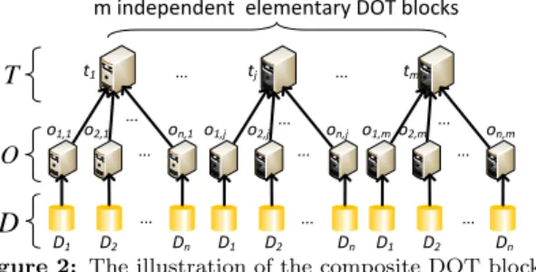
In an elementary DOT block, there is only one worker performing last-stage transformations to update results on intermediate results. It is natural to use multiple workers to collect intermediate results and perform last-stage data transformation, because either intermediate results tend to be huge, or the cardinality of the set of categories of inter-mediate results is greater than one.Thus, a group of inde-pendent elementary DOT blocks is needed, which we define as a composite DOT block, the extension of the elemen-tary DOT block. A composite DOT block is organized by a group of independent elementary DOT blocks, which have the identical worker set of the O-layer and share the same big data (multi-)set as input divided in an identical way. Suppose that a composite DOT block is organized bym el-ementary DOT blocks, each of which hasnworkers in the O-layer. This composite DOT block will combine these ele-mentary DOT blocks (trees) and then form a forest structure shown in Figure 2. Each worker in the O-layer will havem operators, and operatoroi,j means that this operator orig-inally belongs to the worker i of the jth elementary DOT block. The T-layer of this composite DOT block will have mworkers and operatortj means that it is the operator for last-stage transformations of thejth elementary DOT block.
... ... ... ... ... ... o1,1 ... ... o2,1 on,1 o1,j o2,j on,j o1,mo2,m on,m t1 tj tm ... ... ...
m independent elementary DOT blocks
D1 D2 Dn D1 D2 Dn D1 D2 Dn
O T
D
Figure 2: The illustration of the composite DOT block Based on the definitions of the composite DOT block, there are three restrictions on communications among work-ers:
1. workers in the O-layer cannot communicate with each other;
2. workers in the T-layer cannot communicate with each other; and
3. intermediate data transfers from workers in the O-layer to their corresponding workers in the T-layer are the only communications occurring in a composite DOT block.
An example using one composite DOT block is a job used to calculate the sum of even numbers and odd numbers from a large collection of integers. Similar to the example shown in Section 2.1, this large collection of integers is partitioned to nchunks. Two elementary DOT blocks can be used to finish this job, one elementary DOT block for calculating the sum of even numbers and another for calculating the sum of odd numbers. In the elementary DOT block for calculating the sum of even/odd numbers, each worker in the O-layer will first filter out odd/even numbers and calculate the local sum of even/odd numbers as the intermediate result; then, a single worker will collect all intermediate results and calcu-late the sum of even/odd numbers. A composite DOT block is organized by these two elementary DOT blocks. In the T-layer of this composite DOT block, there are2 workers. Operatort1can generate the sum of even numbers, whilet2 can generate the sum of odd numbers.
In a composite DOT block, the execution of its m ele-mentary DOT blocks is flexible. For any two eleele-mentary DOT blocks of those melementary DOT blocks, these two elementary DOT blocks can be executed concurrently or se-quentially, depending on specific system implementations.
2.3
Big Data Analytics Jobs
In the DOT model, a big data analytics job is described by its dataflow, global information and halting conditions.
Dataflow of a Job: The dataflow of a big data analyt-ics job is represented by a specific or non-specific number of elementary/composite DOT blocks. For the dataflow of a big data analytics job, any two elementary/composite DOT blocks are either dependent or independent. For two ele-mentary/composite DOT blocks, if the result generated by a DOT block is directly or indirectly consumed by another DOT block, i.e. one DOT block must be finished before an-other, they are dependent, otherwise they are independent. Independent elementary/composite DOT blocks can be ex-ecuted concurrently.
Global Information: Workers in an elementary/composite DOT block may need to access some lightweight global in-formation, e.g. system configurations. In the DOT model, the global information is available in a common place, such as the coordinator or the global master of the distributed systems. Every worker in an elementary/composite DOT block can access the global information at any time.
Time Global Information
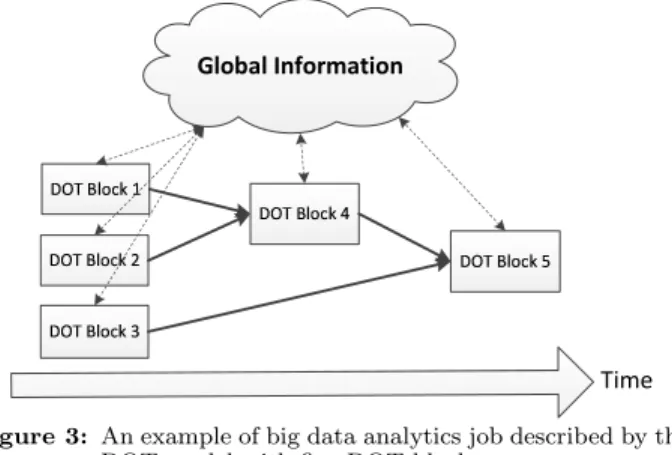
Figure 3: An example of big data analytics job described by the DOT model with five DOT blocks
Global Information Stop? Halting Conditions Yes No DOT Block D O-layer T-layer D
Figure 4: An iterative job described by the DOT model with non-specific number of DOT blocks
Halting Conditions: The halting conditions determine when or under what conditions a job will stop. If a job is represented by a specific number of elementary/composite DOT blocks, the job simply stops after finishing the given number of blocks. In this case, no specific halting condition is needed. For a job represented by a recurrence relation [2], one or multiple conditions must be given, so the application can determine if this job should stop. For example, con-vergence conditions and a maximum number of iterations are two commonly used halting conditions in iterative algo-rithms, such as PageRank [24] and the k-means algorithm [3].
Figure 3 shows an dataflow example described in the DOT model with five DOT blocks. In this example, DOT blocks 1, 2 and 3 process the input data first. Then, DOT block 4 will consume the results generated by DOT blocks 1 and 2. Finally, DOT block 5 will take results of DOT blocks 3 and 4 as its input and generate the final result. The global information can be accessed or updated by all of these five DOT blocks. Because this job will stop after the DOT block 5 stops, there is no halting condition needed.
Figure 4 shows an iterative job described in the DOT model with a non-specific number of DOT blocks. In this example, operators in the O-layer and T-layer of the DOT block in each iteration are the same. After every iteration, halting conditions will be evaluated. If all of the halting con-ditions are true, this job will stop. Similar to the previous example, the global information can be accessed or updated by the DOT block in this iterative job.
2.4
Formal Definitions
In the DOT model, the elementary/composite DOT block can be formally defined using a matrix representation. The dataflow of a big data analytic job involving a specific or non-specific number of DOT blocks is represented by an ex-pression, called a DOT exex-pression, which is defined by an algebra.
2.4.1
The Elementary DOT Block
In the DOT model, the elementary DOT block is formally defined in a matrix representation involving three matrices. The big data (multi-)set is represented by adata vectorD~ =
D1 · · · Dn, whereDiis a chunk. Symboloidenotes the operator of worker iin the O-layer (middle-layer of Figure 1) for processingDi. Operatorso1toonwill form matrixO to representnconcurrent operations onnchunks.
The T-layer (top-layer of Figure 1) is represented by an-other matrix called T, which has one element representing operator t of the single worker for the last-stage transfor-mations based on intermediate results. Note that t is an n-ary function withninputs. The output of an elementary DOT block is still a data (multi-)set and the dimension of the data vector representing the output is1×1. The matrix representation of the elementary DOT block is formulated as: ~ DOT = D1 · · · Dn o1 o2 .. . on t = n F i=1 (oi(Di)) t = t(o1(D1),· · ·, on(Dn)).
In the above matrix representation, matrix multiplication follows the row-column pair rule of the conventional matrix product. The multiplication of corresponding elements of the two matrices is defined as: (1) a multiplication between a data chunkDi and an operatorf (f can either be the op-erator in matrixOor the one in matrixT) means to apply the operator on the chunk, represented by f(Di); (2) mul-tiplication between two operators (e.g. f1×f2) means to form a composition of operators (e.g., f =f2(f1)). In con-trast to the original matrix summation, in the DOT model, the summation operatorPis replaced by a group operator F
. The operation Fn
i=1
(fi(Di)) = (f1(D1),· · ·, fn(Dn))means to compose a collection of data setsf1(D1)tofn(Dn). It is not required that all elements of the collection locate in a single place.
2.4.2
The Composite DOT Block
Given m elementary DOT blocksDO~ 1T1 to DO~ mTm, a composite DOT blockDOT~ is formulated as:
m ⊎ j=1( ~ DOjTj) =DO~ 1T1⊎. . .⊎DO~ mTm=DO~ compositeTcomposite = D1 · · · Dn o1,1 o1,2 · · · o1,m o2,1 o2,2 · · · o2,m .. . ... . .. ... on,1 on,2 · · · on,m t1 0 · · · 0 0 t2 · · · 0 .. . ... . .. ... 0 0 · · · tm = n F i=1 (oi,1(Di)) · · · n F i=1 (oi,m(Di)) t1 0 · · · 0 0 t2 · · · 0 .. . ... . .. ... 0 0 · · · tm = t1(o1,1(D1),· · ·, on,1(Dn)) · · · tm(o1,m(D1),· · ·, on,m(Dn))) , where the operatorUmeans to construct a composite DOT block from m elementary DOT blocks by: (1) using one data vector that includes all chunks used by them elemen-tary DOT blocks and each chunk occurs exactly once; (2) putting matrixOi(column vector) in theith column of the matrixOcomposite; and (3) putting the single element of
ma-trixTi in the place(i, i) of matrixTcomposite. The output of a composite DOT block is still a data (multi-)set and the dimension of the data vector representing the output is 1×m. Details about operator Uare given in section 2.4.3. Moreover, operator “0” will produce an empty set, i.e. given a chunkD,0(D) =∅andDF
∅=D.
2.4.3
An Algebra for Representing the Dataflow of
Big Data Analytics Jobs
With the definition of elementary and composite DOT blocks, the dataflow of a big data analytics job can be sys-tematically represented by a combination of multiple ele-mentary and/or composite DOT blocks. We introduce an al-gebra among elementary and composite DOT blocks. With this algebra, a big data analytics job can be represented by an expression, called aDOT expression. For example, a job can be composed by three composite DOT blocks,
~
D1O1T1,D~2O2T2andD~3O3T3, where the results ofD~1O1T1 andD~2O2T2are input ofD~3O3T3. With the algebra defined in this section, the DOT expression of this job is
(D~1O1T1⊕D~2O2T2)O3T3, whereD~3= (D~1O1T1L~
D2O2T2).
In the DOT model, an elementary/composite DOT block can be viewed as a data vector. In the algebra for DOT expressions, operands are data vectors, elementary DOT blocks and composite DOT blocks. The algebra defines two basic interactions between two DOT blocks, as shown by the above simple example, the interaction between two in-dependent DOT blocks and that between two in-dependent DOT blocks. If two DOT blocks do not have data depen-dency, they are independent DOT blocks; otherwise, they are dependent DOT blocks. There are two operations to define the interaction among independent DOT blocks for DOT expressions:
• L: For two data vectors~
D1=D1,1 D1,2 · · · D1,n andD~2= D2,1 D2,2 · · · D2,m, ~ D1⊕D~2= h ~ D1 D~2 i = D1,1 D1,2 · · · D1,n D2,1 D2,2 · · · D2,m. The operatorL simply collects all chunks and forms a new data vector of a higher dimension. For two ele-mentary/composite DOT blocks DOT blocksD~1O1T1 andD~2O2T2, ~ D1O1T1⊕D~2O2T2= h ~ D1 D~2 iO 1 0 0 O2 T1 0 0 T2 . For a data vector D~1 and an elementary/composite DOT blockD~2O2T2, ~ D1⊕D~2O2T2= h ~ D1 D~2 iI 0 0 O2 I 0 0 T2 , of which I is an identity matrix. Here, an identity matrix is a matrix with the operator “1”(s) on the main diagonal and the operator “0”(s) elsewhere. For a given chunkDi, operator “1” is defined as1(Di) =Di. Thus, for a given 1×ndata vector D~ and a n×nidentity matrixI,DI~ =D~.
• U: For two data vectors~
D1=D1,1 D1,2 · · · D1,n andD~2= D2,1 D2,2 · · · D2,m, ~ D1⊎D~2 = D1,1 D1,2 · · · D1,n D2,q1 D2,q2 · · · D2,qk , where k ≤m, 1 ≤q1 < q2 < . . . < qk−1 < qk ≤ m and for each i (1 ≤ i ≤ k), D2,qi ∈/
S
1≤i≤n
D1i. Like the operator L, operator U also combines multiple data vectors into a single data vector of higher di-mension, and to combine multiple independent ele-mentary/composite DOT blocks into one composite DOT block. However, after the operation ofU
, each common chunk used by multiple independent elemen-tary/composite DOT blocks occurs exactly once. For matricesOandT in the new composite DOT block, op-erators will simply be assigned to match the new data vector. We use two examples to explainU
operators. Consider that the data vectors in these two examples areD~1=
D1 D2andD~2=D1 D3. For two data vectors D~1 and D~2, D~1U~
D2 =D1 D2 D3. Con-sider two elementary/composite DOT blocks,D~1O1T1 andD~2O2T2, of which O1= o1,1,1 o1,1,2 o1,2,1 o1,2,2 T1= t1,1 0 0 t2,2 O2= o2,1,1 o2,1,2 o2,2,1 o2,2,2 T2= t2,1 0 0 t2,2 . The result ofD~1O1T1U~ D2O2T2is: ~ D1O1T1⊎D~2O2T2 = D1 D2 D3 o1,1,1 o1,1,2 o2,1,1 o2,1,2 o1,2,1 o1,2,1 0 0 0 0 o2,2,1 o2,2,2 t1,1 0 0 0 0 t1,2 0 0 0 0 t2,1 0 0 0 0 t2,2 .
For two dependent DOT blocks, these two DOT blocks will be chained together according to the data dependency, e.g.(DO1T1)O2T2. Two dependent DOT blocks can be merged into one DOT block in a certain condition, described by the property ofconditional associativity.
Property 2.1. conditional associativity:If matrixO in a composite DOT block is a diagonal matrix, this compos-ite DOT block can be merged into matrix T of its preceding composite DOT block or into matrixOof its succeeding com-posite DOT block.
For example, there are two dependent DOT blocks, described by (DO1T1)O2T2= (D1 D2 o1,1,1 o1,1,2 o1,2,1 o1,2,2 t1,1 0 0 t2,2 ) o2,1,1 0 0 o2,2,2 t2,1 0 0 t2,2 .
Based on the property ofconditional associativity, these two DOT blocks can be merged into one DOT block, which is D1 D2 o1,1,1 o1,1,2 o1,2,1 o1,2,2 t2,1(o2,1,1(t1,1)) 0 0 t2,2(o2,2,2(t2,2)) . With the above algebra, the dataflow of a big data ana-lytics job can be described by a DOT expression composed by data vector, elementary/composite DOT block, operator L
and/or operator U
. A context-free grammar to derive a DOT expression is shown in Figure 5.
hDOTexpressioni→hdataVectori
hdataVectori→hDi|(hDi)|hdataVectorihOihTi|
(hdataVectorihOihTi)|
hDi⊕hdataVectori|(hDi⊕hdataVectori)| hDi⊎hdataVectori|(hDi⊎hdataVectori)|
hDihOihTi⊕hdataVectori|(hDihOihTi⊕hdataVectori)| hDihOihTi⊎hdataVectori|(hDihOihTi⊎hdataVectori)
hDi→a data vector D~ hOi→aOmatrix hTi→aT matrix
Figure 5: The context-free grammar of the DOT expression If the dataflow of a job needs a non-specific number of elementary/composite DOT blocks, such as an iterative al-gorithm for a PageRank evaluation [24], the dataflow should be described by a recurrence relation. The general format of a DOT expression representing a recurrence relation is:
~ D(t) = j L k=i ~
D(k)O(k+ 1)T(k+ 1),0≤i≤j < t. For example, a recurrence relationD(t) =~ D(t~ −1)O(t)T(t)means at timet, the result is generated byD(t~ −1)O(t)T(t), of whichD(t~ −1) is the output at timet−1.
With the algebra used for representing the dataflow of a big data analytics job as a DOT expression, the job can be described by a DOT expression, global information and halting conditions.
2.5
Restrictions
To make the DOT model effective in practice, we add several restrictions.
The power of workers: In big data analytics, it is rea-sonable to assume there is no single worker that can store the entire data (multi-)set. Thus, similar to [18], we restrict that the storage capacity of a single worker is sublinear to the size of data. We do not set any restriction on the com-putation power of a single worker, which mainly determines the elapsed time of an operator on a single worker.
The number of workers: In big data analytics, it is reasonable to assume the total number of workers in matrix Oor matrixT is much smaller than the size of the data. For matricesOandT in a DOT block, we assume that the total number of workers is sublinear to the size of data.
3.
SCALABILITY AND FAULT-TOLERANCE
Scalability and fault-tolerance are two critical issues in big data analytics. In this section, we show that the processing paradigm of the DOT model is scalable and fault-tolerant.
3.1
Scalability
There are five concepts needed to be defined at first. Definition 3.1. A minimum chunk is defined as a chunk that cannot be further divided into two chunks. A minimum chunk represents a operator-specific collection of data that has to be processed by a single operator at a single place during a continuous time interval.
Definition 3.2. A basic concurrent data process-ing unitis defined as a worker which only processes a min-imum chunk.
Definition 3.3. A processing stepis defined as a set of data operations being executed on a fixed number of con-current workers during a continuous time interval.
Definition 3.4. Scalability of a job: The scalability of a job is defined by two aspects:
1. with a fixed input data size N0, the throughput of this job linearly increases as the number of workers involved in each processing step of this job linearly increases at ratio γ (an integer). This linear increase of the throughput stops when there exists a processing step, where each worker is reduced to a basic concurrent data processing unit; and
2. with an initial input data sizeN0, as the input data size increases linearly at ratio ω and thus the input data size is ωN0, the elapsed time of this job can be kept constant by increasing the number of workers involved in this job at ratioγ.
Definition 3.5. Scalability of a processing paradigm:
Given a job classAthat all job of this class satisfy two condi-tions: (1) the time complexity of operations on every worker is Θ(n), where nis the size of the input data; and (2) the input data of a processing step can be equally divided into multiple data sub-sets. Also, suppose that the point-to-point throughput of the network transfer between two workers will not drop when adding more workers.
A processing paradigm is scalable if any job of the classA represented by this processing paradigm is scalable.
With the above five definitions, we will show that the processing paradigm of the DOT model is scalable.
Lemma 3.1. The processing paradigm of the DOT model is scalable.
Proof. Firstly, we prove that any job of the classA rep-resented by a single DOT block is scalable. Consider a job represented by a single DOT block, which is
~ DOT= D1 · · · Dn o1,1 · · · o1,m .. . . .. ... on,1 · · · on,m t1 · · · 0 .. . . .. ... 0 · · · tm ,
wherenandmare the initial number of workers in matrices OandT, respectively. Based on the definition of a processing step, there are two processing steps represented by matrices O andT, respectively. The throughput of this DOT block is represented asT hroughput= ωN0
Telapsed. TheTelapsedis the
elapsed time of this DOT block and
Telapsed=ωtO,n+ωtT,m+f(ωN0, n, m),
of whichtO,nis the elapsed time of matrixOwithnworkers (the longest elapsed time of operation execution among all workers in matrixO),tT,m is the elapsed time of matrix T withmworkers (the longest elapsed time of operation exe-cution among all workers in matrix T), andf(ωN0, n, m) is the elapsed time of network transfer from workers in matrix O to workers in matrix T with the input data sizeωN0,n workers inOandmworkers inT.
If the input data size is fixed as N0, ω will be constant value 1. The linear increase of workers by a factor of γ means that matrix Owill haveγnworkers andT will have γmworkers. This increase of worker can be done as follows: for every 3-tuple (Di, oi,j, tj), where Di ∈ D~, oi,j ∈ O and tj∈T
• oi,j in matrixOwill be replaced by oi,j1,1 · · · oi,j1,γ .. . . .. ... oi,jγ,1 · · · oi,jγ,γ ;
• tj in matrixT will be replaced by tj1 · · · 0
..
. . .. ... 0 · · · tjγ .
Here, for a givenγ,Diwill be equally divided intoDi
1,· · ·, Dγi. For example, for a composite DOT block
~ DOT= D1 D2 o1,1 o1,2 o2,1 o2,2 t1 0 0 t2 ,
with2 workers in matrix O,2 workers in matrix T, and a worker-increase factor γ of 2, the new DOT block D~′O′T′
representing4workers inOand4workers inT will be
~ D′O′T′= D11 D12 D21 D22 o1,11,1 o1,11,2 o1,21,1 o1,21,2 o1,12,1 o1,12,2 o1,22,1 o1,22,2 o2,11,1 o2,11,2 o2,21,1 o2,21,2 o2,12,1 o2,12,2 o2,22,1 o2,22,2 t11 0 0 0 0 t12 0 0 0 0 t21 0 0 0 0 t22 .
With this method, the elapsed time of matrix O, T and network transfer will decrease linearly, i.e. tO,γn = tO,nγ , tT,γn =
tT ,n
γ and f(N0, γn, γm) = f(N0γ,n,m). Thus, the elapsed time of this DOT block will be
Telapsed=tO,n γ + tT,m γ +f(N0, γn, γm) = 1 γC, of whichCis constant value toγ. So, the throughput of this DOT block is
T hroughput=N0 C γ,
whereN0andCare constant values toγ. When every worker in eitherOorT only processes the minimum chunk defined by the application, i.e. every worker is reduced to a basic concurrent data processing unit, the number of workers of this DOT block cannot be further added to gain linear in-crease of the throughput. Thus, with a fixed input data size, the throughput of the DOT block linearly increases as the number of workers linearly increases until there is a processing step, each worker of which is reduced to a basic concurrent data processing unit.
If the the data size increases linearly, the number of work-ers in two matrices can be scaled with the same method provided above and the elapsed time of network transfer will be proportional to the ratioωtoγ, i.e.f(ωN0, γn, γm) = ω
γf(N0, n, m). So the elapsed time of the DOT block is Telapsed=ωtO,n γ +ω tT,m γ +f(ωN0, γn, γm) = ω γC, of which C is a constant value to ω and γ. Thus, if ω
γ is a constant, theTelapsed will be a constant value and then
the job elapsed time can be kept constant by increasing the number of workers linearly.
For a big data analytics job of the classAexpressed by a DOT expression, a matrixOorT will represent a processing step. The conclusion that a job of class Arepresented by a DOT expression is scalable is a corollary of the fact that a job of classArepresented by a DOT block is scalable.
Thus, the processing paradigm of the DOT model is scal-able.
3.2
Fault-Tolerance
Here are four basic concepts to be used in the rest of this sub-section.
Definition 3.6. Initial input data is defined as the available data to be accessed in an archived storage at the start of a set of concurrent operations.
Definition 3.7. Runtime data is defined as the data generated during the runtime of a set of concurrent opera-tions.
Definition 3.8. Fault-tolerance of a job: Assuming the initial input data of every operator is always available, a big data analytics job is fault-tolerant if it can finish and generate a correct result when worker failures happen. The result of a job involving worker failures is correct if and only if the result is identical to one of the possible results gener-ated by this job without worker failures.
Definition 3.9. Fault-tolerance of a processing paradigm:
A processing paradigm is fault-tolerant if any job represented by this processing paradigm is fault-tolerant.
With the above four definitions, we will show that the processing paradigm of the DOT model is fault-tolerant.
Lemma 3.2. The processing paradigm of the DOT model is fault-tolerant.
Proof. Consider a job represented by a DOT block with nworkers in matrixOandmworkers in matrixT, and con-sider that there arek1(1≤k1≤n) failed workers inOand k2 (1 ≤ k2 ≤ m) failed workers in T during the job exe-cution. Because the DOT model enforces that there is no data dependency among peer workers in matrixOand those in matrixT, which is reflected by the interactions between matrices O and T, new workers to substitute the services of failed workers will only be started to re-execute opera-tors running on the failedk1workers inOandk2workers in T. Since the initial input data of every operator is always available, there is no difference on functionalities between a substitute worker and an original worker. Thus, a DOT block is fault-tolerant.
For a big data analytics job expressed by a DOT expres-sion composed by a specific or non-specific DOT blocks, because any DOT block of this DOT expression is tolerant, the job expressed by this DOT expression is fault-tolerant.
Since any job represented by the processing paradigm of the DOT model is fault-tolerant, the processing paradigm of the DOT model is fault-tolerant.
4.
OPTIMIZATION RULES
We identify three types of framework and implementa-tion independent optimizaimplementa-tion rules under the DOT model.
These three types of rules can be applied on various frame-works to optimize the performance of big data analytics jobs. To be concise and without loss of generality, we use two com-posite DOT blocks as examples to explain these three types of optimization rules in this section. These two composite DOT blocks are defined as follows:
blocki=D~iOiTi= Di,1 Di,2 oi,1,1 oi,1,2 oi,2,1 oi,2,2 ti,1 0 0 ti,2 , i= 1,2.
4.1
Preliminary Definitions
Here are four definitions to be used in the rest of this section.
Definition 4.1. Equivalence between two data vec-tors: Two data vectors D1 =~
D11 · · · D1n and D2 =~
D21 · · · D2m are equivalent, denoted as D1~ ≡ D2~ , if and only if S
1≤i≤n
D1i= S 1≤i≤m
D2i.
Definition 4.2. Equivalence between two DOT blocks:
Two elementary/composite DOT blocksDo1 =~ D1O~ 1T1and ~
Do2 =D2O~ 2T2are equivalent, denoted asD1O~ 1T1≡D2O~ 2T2, if and only ifD1~ and D2~ are equivalent, and Do1~ andDo2~ are equivalent.
Definition 4.3. Equivalence between two DOT ex-pressions: Two DOT expressions EXP1 and EXP2, are equivalent, denoted asEXP1≡EXP2, if and only if
⊕ 1≤i≤n ~ D1inputi≡1≤⊕ i≤m ~ D2inputi and ⊕ 1≤i≤n ~ D1outputi≡ ⊕ 1≤i≤m ~ D2outputi, of which (1)D1~ input i(i= 1, . . . , n) andD2~ inputi (i= 1, . . . , m) are the original input ofEXP1 andEXP2, respectively, and (2)D1~ output
i (i= 1, . . . , n) andD2~ outputi (i= 1, . . . , m) are the final output ofEXP1 andEXP2, respectively.
Definition 4.4. Associative-decomposable operators:
As defined in [28], an operatorHis associative-decomposable if it can be decomposed into two operatorsF andC so that:
1. ∀D1, D2, H(D1⊕D2) =C(F(D1)⊕F(D2));
2. F andC are commutative, i.e.∀D1, D2, F(D1⊕D2) = F(D2⊕D1), C(D1⊕D2) =C(D2⊕D1);and
3. Cis associative, i.e.∀D1, D2, D3, C(C(D1⊕D2)⊕D3) = C(D1⊕C(D2⊕D3)).
4.2
Substituting Expensive Remote Data
Trans-fers with Low-Cost Local Computing
In the DOT model, there is no restriction on the amount of data transfers in the communication phase, because the amount of data transfers is application dependent. Some ap-plications may need to transfer a large amount of data, while others may only need to transfer a small amount. However, considering the fact that “Computing is free” and “Network traffic is expensive” [14], application designers should mini-mize the amount of remote data transfers in practice.In an elementary/composite DOT block, an associative-decomposable operator in matrixT can transfer partial op-erations to matrixO. Associative-decomposable operators which originally belong to the same elementary DOT block, i.e. these operators locate in the same column of the ma-trixO, can transfer common-partial operations to matrixT. With the definition of equivalence between two DOT blocks,
an elementary/composite DOT block can be transformed to an equivalent one. For example, if inblock1, operatort1,1 is associative-decomposable and can be decomposed into two operatorsF andC, the equivalent composite DOT block of block1will be:
block1≡block′1= D1,1 D1,2 F(o1,1,1) o1,1,2 F(o1,2,1) o1,2,2 C 0 0 t1,2 . Moreover, if the amount of intermediate results generated by F(o1,1,1)andF(o1,2,1)is less than that generated byo1,1,1 ando1,2,1, the total amount of data transfered will decrease. Thus, the expensive remote data transfers are replaced by an additional low cost local computationsF. For example, considering an application that counts the number of occur-rences of each word in a large number of documents or web pages. A simple way to implement this application is to let operators in matrixOemit a pair(word, 1)for every word. Then, we use a hash partitioning function to decide which worker in matrixT a pair will be sent to. Finally, workers in matrix T calculate the number of occurrences for each word. There is a aggregation operatorF that will accumu-late the value for pairs with the same key, i.e. generate a pair
(word, local count) for each word. If this operatorF is ap-plied locally to all operators in matrixO, each worker in the new matrixOonly emits pairs with accumulated number of occurrences for each word. By introducing the operatorF, the total amount of intermediate results transferred through networks will be significantly reduced and thus the execution time of this job will decrease. In the MapReduce framework, this operatorFcan be implemented by theCombiner Func-tion[11].
4.3
Exploiting Sharing Opportunities among
Composite DOT Blocks
Exploiting sharing opportunities has been studied by the database community in different contexts, e.g. [21], [8] and [9].Based on the DOT model, we identify three types of shar-ing opportunities among two independent composite DOT blocks,block1andblock2, and introduce how to exploit these three types of sharing opportunities. In this sub-section, we consider that the dataflow of a job isblock3=block1⊎block2.
Sharing Common Chunks: Ifblock1 and block2 share a common chunk, e.g. suppose D1,1 = D2,1, the result of block1⊎block2will be:
block3=block1⊎block2
= D1,1 D1,2 D2,2 o1,1,1 o1,1,2 o2,1,1 o2,1,2 o1,2,1 o1,2,2 0 0 0 0 o2,2,1 o2,2,2 t1,1 0 0 0 0 t1,2 0 0 0 0 t2,1 0 0 0 0 t2,2 .
Because the decision of how to execute operators in a worker is flexible, when operators in a worker share a single scan of the chunk, sharing common chunks will reduce the local disk I/O.
Sharing Common Operations in Matrix O: After sharing the common chunks, if two operators in different columns of matrix O have common operations, these two columns can be merged. Suppose thato1,1,1ando2,1,1are common operations, so a new operatoro′can represent both operators of o1,1,1 and o2,1,1. Thus, block3 will be trans-formed to a new composite blockblock′
toblock3. The DOT blockblock3′ will be block3′ = D1,1 D1,2 D2,2 o′ o 1,1,2 o2,1,2 o1,2,1 o1,2,2 0 o2,2,1 0 o2,2,2 (t1,1, t2,1) 0 0 t1,2 0 0 0 t2,2 ,
of which operator(t1,1, t2,1)means to generate two outputs, one for operator t1,1 and another for operator t2,1. The benefit of sharing common operators in matrix Ois to re-duce redundant processing operations, which will decrease elapsed time.
Sharing Common Operations in Matrix T: After sharing common operations in matrixO, an equivalent com-posite DOT block block′
3 is created. If in the DOT block block′
3,t1,1andt2,1 have common operations, a new opera-tort′ can represent both operatorst
1,1 andt2,1. Thus, in block′
3, operatort′will replace operator(t1,1, t2,1).
4.4
Exploiting the Potential of Parallelism
In this sub-section, we consider thatblock1andblock2are dependent and suppose thatblock1is the input ofblock2, i.e.
~
D2 = D~1O1T1. If O2 is a diagonal matrix, i.e.o2,1,2 = 0 ando2,2,1= 0, the intermediate results ofblock2do not need to be redistributed in the network. According to Property 2.1 in Section 2.4.3,O2T2 can be merged into matrixT1of block1. Thus, the newblock1is:
block′1=D~1O1T1′ = D1,1 D1,2 o1,1,1 o1,1,2 o1,2,1 o1,2,2 t2,1(o2,1,1(t1,1)) 0 0 t2,2(o2,2,2(t1,2)) . With this optimization, for a job composed by D~1O1T′
1, once intermediate results generated byD~1O1 are collected by workers inT1′, each workers will process its data in paral-lel till the end of this job. This optimization will eliminate the time spent on launching theblock2, and storing and col-lecting intermediates results generated by workers in matrix O2. Thus, the elapsed time ofblock′1=D~1O1T1′ is less than that of runningblock1 andblock2one by one.
5.
EFFECTIVENESS OF THE DOT MODEL
In this section, we demonstrate the effectiveness of the DOT model with four types of case studies: (1) Certi-fication: certifying the scalability and fault-tolerance of processing paradigms of software frameworks; (2) Evalu-ation and Comparison: evaluating and comparing soft-ware frameworks; (3)Optimization: optimizing job per-formance on various software frameworks; and (4) Simu-lation: providing a simulation-based framework for cost-effective software design.
5.1
Certification
The DOT model can be used to certify the scalability and fault-tolerance of the processing paradigm of a software framework for big data analytics.
Lemma 5.1. For a software frameworkF for big data an-alytics, if any job ofF can be represented in the DOT model by either a single DOT block or a DOT expression, the pro-cessing paradigm of this frameworkF is scalable and fault-tolerant.
Proof. For a given software framework F for big data analytics, if any job of it can be represented in the DOT model, the processing paradigm is regulated by the process-ing paradigm of the DOT model. Based on the Lemma 3.1 and Lemma 3.2, the processing paradigm of this software frameworkF is scalable and fault-tolerant.
With Lemma 5.1, we can study the scalability and fault-tolerance of the processing paradigms of different big data analytics frameworks. In this sub-section, we use two widely-used software frameworks, MapReduce [11] and Dryad [17], as case studies.
5.1.1
MapReduce
A MapReduce job has threeuser-defined functions, map
function, partitioning function and reduce function. The worker running themap/reducefunction is calledmap worker/
reduce worker. Every map function processes each input key/value pair provided from an underlying distributed file system and produces a set of intermediate key/value pairs. The partitioning function will decide which reduce worker an intermediate key/value pair will be sent to. Then, the MapReduce framework willshuffleintermediate results through the network and merge all intermediate key/value pairs based on the key. Finally, for every intermediate key and its values, the reduce function will generate the final results.
A computation model of the MapReduce framework is proposed by [18], in which a big data analytics job is com-posed of a sequence of MapReduce jobs. This model re-quires that the map function is stateless and the key/value pairs generated by a reduce function will have the same key with the intermediate key fed to this reduce function. In this paper, we take this model to represent the MapReduce. However, considering its practical usage, we slightly extend the power of map workers and reduce workers. Map workers can have stateful map functions, but a map worker only re-members key/value pairs it has processed. Moreover, based on the intermediate key and its values, a reduce function of a reduce worker can generate a sequence of new key/value pairs, of which new keys differ from the intermediate key.
To certify that the processing paradigm of the MapReduce framework is scalable and fault-tolerant, using Lemma 5.1 as a basis, we need to show that any MapReduce job can be represented by the DOT model.
Lemma 5.2. Any MapReduce job can be represented by a single DOT block.
Proof. A MapReduce job can be represented by an ele-mentary or composite DOT block as follows:
~ DOT= D1 · · · Dn p1(omap) · · · pm(omap) .. . . .. ... p1(omap) · · · pm(omap) treduce · · · 0 .. . . .. ... 0 · · · treduce ,
where matrix O represents the map phase, T represents the reduce phase and the multiplication between DO~ and matrix T represents the shuffle phase. The data vector
~
D =
D1 D2 · · · Dn represents the partitioned input data. Operatoromap means to apply the map function on each record of the input data. Operatorpirepresents apply-ing a partitionapply-ing function on each intermediate key/value
pair generated byomap and then extracting all intermedi-ates key/value pairs which will be sent to the ith reduce worker represented by rowiin the matrixT. Finally, opera-tortreducewill first merge intermediate key/value pairs into groups based on the key and then apply the reduce function on each group. Thus, a MapReduce job can be represented by an elementary or composite DOT block.
Based on Lemma 5.2, we can then claim that the process-ing paradigm of the MapReduce framework is scalable and fault-tolerant.
Lemma 5.3. The processing paradigm of the MapReduce framework is scalable and fault-tolerant.
Proof. It is the corollary of Lemmas 5.1 and 5.2.
5.1.2
Dryad
In Dryad, the dataflow of a big data analytics job is rep-resented by a directed acyclic graph (DAG)
G=< VG, EG, IG, OG>,
whereVG contains all vertices,EG contains all edges,IG⊆ VG contains all inputs, and OG⊆VG contains all outputs. In a DAG, there are two kinds of vertices representing data on an underlying distributed file system and operations of data processing, respectively. The edge represents the com-munication among workers.
To certify that the processing paradigm of the Dryad frame-work is scalable and fault-tolerant, we need to show that any Dryad job can be represented by the DOT model.
Lemma 5.4. A Dryad job represented by a DAG can be represented by a DOT expression.
Proof. We give the method used to write a DOT expres-sion for a given DAG in Dryad. Given a DAG
G=< VG, EG, IG, OG> and its graph of job stages
Gs=< VGs, EGs, IGs, OGs >,
the procedure of representing this DAG by a DOT expres-sion is shown as follows.
1. Initialize a setSto∅. This set contains the enumerated vertices inGs. Initialize a setU toVG. The set ofU contains the vertices that have not been enumerated inGs;
2. Find a vertex v in U, which does not have incoming edge from vertices inU;
(a) Ifv represents input data, find all vertices in G corresponding to v and use a data vector D~ to represent this input data. Then, addvintoSand removevfromU;
(b) If v represents an operation of data processing, create a matrixTnew by using all corresponding operation vertices of v in the set VG as opera-tors of diagonal matrixTnew. Based onEGs, find all corresponding vertices inSpointing tov and denote the set of these vertices asP. Then, ap-plyLto the DOT blocks or data vectors repre-senting source vertices inP to create a new data vectorD~new. Based on the composition of edges from vertices ofP tov(pointwise composition or complete bipartite graph), create a matrixOnew, each element of which is either operator 1 or 0.
This matrix Onewis used to represent the edges from vertices in P to v. Then, create a new ele-mentary/composite DOT block,D~newOnewTnew. Finally, addvintoSand removevfromU; (c) Ifvrepresents output data, go to the next step; 3. If all vertices inUare those vertices representing
out-put data, go to step 4. Otherwise, go to step 2; 4. Use Property 2.1 to simplify the DOT expression; 5. Till this step, a DOT expression is created for the DAG
G. The result of this DOT expression is the output of the DAG;
Thus, a Dryad job can be represented by a DOT expres-sion.
Based on Lemma 5.4, we have shown that the process-ing paradigm of the Dryad framework is scalable and fault-tolerant.
Lemma 5.5. The processing paradigm of the Dryad frame-works is scalable and fault-tolerant
Proof. It is the corollary of Lemma 5.1 and 5.4.
5.2
Evaluation and Comparison
In Section 5.1, we have shown that any MapReduce/Dryad job can be represented by the DOT model. If both MapRe-duce and Dryad can execute big data analytics jobs repre-sented by the DOT model, the DOT model can server as the bridge for application migration between MapReduce and Dryad. In this sub-section, we evaluate if MapReduce and Dryad can execute big data analytics jobs represented by the DOT model, i.e if MapReduce and Dryad can execute elementary/composite DOT blocks and DOT expressions. Also, since the execution of independent elementary DOT blocks in a composite DOT block is flexible, we will com-pare if MapReduce and Dryad support sharing data scan among operators in the O-layer of a composite DOT block. If both of MapReduce and Dryad can execute big data an-alytics jobs represented by the DOT model and can share data scan among operators in the O-layer of a composite DOT block, these two software frameworks will not display fundamental differences on executing a big data analytics job.
5.2.1
Executing a DOT Block on MapReduce
We first show a general method to execute a DOT block on MapReduce.
Lemma 5.6. A DOT block withnconcurrent workers in matrix Oandmconcurrent workers in matrixT can be ex-ecuted by at mostn×m+m MapReduce jobs, wheren×m concurrent map-only MapReduce jobs represent matrixOin the DOT block andmconcurrent map-only MapReduce jobs represent matrixT.
Proof. In a DOT block, peer workers in matrix O or T do not have data dependency. For every chunk in data vectorD~ =
D1 · · · Dn, there aremoperators to be ap-plied. In the worst case, m map-only MapReduce jobs are needed to process a chunk and then generate m intermedi-ate results formworkers in matrixT. Thus, there aren×m independent map-only MapReduce jobs needed to perform data processing represented by matrixO. Similarly,m inde-pendent map-only MapReduce jobs are needed to perform data processing represented by matrixT. Because indepen-dent MapReduce jobs can be executed concurrently, a DOT
block with n concurrent workers in matrix O and m con-current workers in matrix T can be executed by at most n×m+m MapReduce jobs, wheren×mconcurrent map-only MapReduce jobs represent matrixOin the DOT block andmconcurrent Map-only MapReduce jobs represent ma-trixT.
Although, in the worst case,n×m+mmap-only MapRe-duce jobs are needed to execute a DOT block, if some op-erators can share the data scan in a worker, the number of needed MapReduce jobs for executing this DOT block can be reduced. Consider a DOT block
~ DOT = D1 · · · Dn o1,1 · · · o1,m .. . . .. ... on,1 · · · on,m t1 · · · 0 .. . . .. ... 0 · · · tm ,
and consider two setsR={rp|rp∈ {1,2,· · ·, n}} ⊆ {1,2,· · ·, n} andC={cq|cq∈ {1,2,· · ·, m}} ⊆ {1,2,· · ·, m}. If, for a given i∈R, alloi,j(j∈C) can share the data scan, and for a given j∈C, alloi,jfor everyi∈Rare the same, a single MapRe-duce job can be used to execute operatorsoi,jandtj, where i∈ R and j ∈ C. In this MapReduce job, the map phase will execute operatorsoi,j, where i ∈ Rand reduce phase will execute operators tj, where j ∈ C. The partitioning function will distribute intermediate results from an opera-toroi,j to worker performingtj. Thus, the total number of MapReduce jobs for executing a DOT block can be further reduced.
Since, an elementary/composite DOT block can be exe-cuted by MapReduce jobs and there is an underlying dis-tributed file system associated with the MapReduce frame-work, a DOT expression also can be executed by MapReduce jobs.
5.2.2
Executing a DOT Block on Dryad
We first present a general method to execute a DOT block on Dryad.
Lemma 5.7. A DOT block can be executed by a Dryad job expressed by a DAG.
Proof. Given an arbitrary DOT block ~ DOT = D1 · · · Dn o1,1 o1,2 · · · o1,m o2,1 o2,2 · · · o2,m .. . ... . .. ... on,1 on,2 · · · on,m t1 0 · · · 0 0 t2 · · · 0 .. . ... . .. ... 0 0 · · · tm ,
the corresponding DAG of the Dryad job is shown in Figure 6. In this DAG, verticesD1toDn represent elements of the data vector. Operatoroi,jis the operator at theith row and jcolumn of matrixO. Operator in matrixT are represented byt1totmin the DAG. Thus, a DOT block can be executed by a Dryad job.
If in matrixO, some operators can share the data scan, the DAG can be changed to represent the data scan by merging corresponding vertices, adding new vertices for partitioning intermediate results and adjusting edges accordingly. For example, for every worker, if all operators of a worker in ma-trixOcan share the data scan, i.e. for all rows, all operators in a row can share the data scan, the DAG can be changed to Figure 7. In this DAG,Oi represents all operators of the ith workers in the matrixOand thus it is composed by all
t t Data vector Matrix T Output O O O O Matrix O D D
Figure 6: The DAG of a DOT block
O O p p t t Matrix O Matrix T Output D D Data vector
Figure 7: An example DAG for sharing data scan operators in the ith row, i.e. Oi = (oi,1, . . . , oi,m). Vertices pi (1≤i≤n) are data distribution vertices, each of which will distribute the intermediate results generated byOi to corresponding workers in the matrixT represented by ver-tices t1 to tm in the DAG, i.e. pi is responsible for all oi,j (1≤j ≤m) and for a givenj, pi will distribute results of oi,j totj. Finally,t1totmwill generate the output.
Since, an elementary/composite DOT block can be exe-cuted by Dryad jobs and there is an underlying distributed file system associated with the Dryad framework, a DOT expression also can be executed by a Dryad job.
5.2.3
Discussion
Through 5.2.1 and 5.2.2, we have shown that a DOT block can be executed by MapReduce and Dryad. Also, if oper-ators of a worker in matrixO can share data scan, both of these two frameworks can execute these operators with a single pass of input data. Thus, for a given DOT block, job execution of MapReduce and Dryad are equivalently repre-sented by the DOT model. The core computing flows of MapReduce and Dryad are the same, although implementa-tion details can be different. For a given big data analytics job represented by the DOT model, the processing paradigm of this job will be the same under the MapReduce and Dryad frameworks.
5.3
Optimization
With optimization rules provided in Section 4, the DOT model can be used to optimize big data analytics jobs on var-ious frameworks. Moreover, the optimization made by the DOT model is framework and implementation independent, so the optimization can be automatically ported among frame-works which can execute DOT blocks. In this sub-section, we use a structured data analysis based on SQL conducted on the MapReduce framework as a case study to show the effectiveness of the DOT model in optimizing job execution. In this case, we choose the TPC-H benchmark [4] as the workload, which is a widely used data warehousing bench-mark. Due to the page limit, we only present the perfor-mance evaluation of TPC-H Q17 as a representative case.
1SELECT sum(l_extendedprice) / 7.0 AS avgyearly
2FROM (SELECT l_partkey, 0.2* avg(l_quantity) AS tmp 3 FROM Lineitem
4 GROUP BY l_partkey) AS t1,
5 (SELECT l_partkey,l_quantity,l_extendedprice
6 FROM Lineitem, Part
7 WHERE p_partkey = l_partkey AND
8 p_brand = ’X’ AND
9 p_container = ’Y’) AS t2
10WHERE t2.l_partkey = t1.l_partkey AND
11 t2.l_quantity < t1.tmp;
Figure 8: A flattened variation of TPC-H Q17
Lineitem (L) Lineitem (L) Part (P) AGG1 (A1) JOIN1 (J1) JOIN2 (J2) AGG2 (A2)
Figure 9: Query plan tree of TPC-H Q17
Because the MapReduce framework does not support nested parallelism [16], TPC-H Q17 should be “flattened” so that this query can be implemented in the MapReduce frame-work. The query shown in Figure 8 with the query plan tree shown in Figure 9 is flattened based on first-aggregation-then-join algorithm [19].
In Figure 8, lines 2-4 are for the aggregation operation
AGG1(A1) in the query plan tree, which generates the tem-porary table t1. The join operation JOIN1(J1) between tablesLineitem(L) andPart(P) is shown in lines 5-9. The result ofJ1 is the temporary table t2. Then, JOIN2(J2) will join tablest1andt2. Finally, AGG2(A2) will perform an aggregation on the result ofJ2and output the ending re-sults. In the DOT model, each operation ofA1,J1,J2and
A2can be represented by a composite DOT block. Then, this query can be represented by a DOT expression, which is
Q17 = ((D~LOA1TA1⊕(D~L⊕D~P)OJ1TJ1)OJ2TJ2)OA2TA2. This DOT expression can be implemented by four MapRe-duce jobs. However, considering the optimization opportu-nities analyzed in Section 4, a DOT expression with only two composite DOT blocks can be used for this query. To show the optimization procedure, without loss of generality, we set the dimension of each matrix in the DOT expression based on Table 1. The original DOT expression for TPC-H Q17 is shown in Figure 10, where each operator in matrix Ois combined by an operatoro that simply selects desired records from input data vector and a partitioning operatorp that selects desired output records of operatorofor a worker in matrixT based on hash values of those records. For ex-ample, if the hash value of a output record of operatorois 1, this output record will be collected by the first worker in matrixT and thus, only partitioning operatorpat first col-umn of matrixOwill select this record; Moreover, in Figure 10, an operator in matrixT will performaggregationorjoin
operations.
The optimization procedure has three steps:
1. BecauseA1 andJ1share common chunks, we can
Table 1: The dimension of each matrix in the DOT expression of TPC-H Q17
Matrix Dimension Matrix Dimension ~ DL 1×2 D~P 1×2 OA1 2×2 OJ2 4×2 TA1 2×2 TJ2 2×2 OJ1 4×2 OA2 2×2 TJ1 2×2 TA2 2×2
substitute the operator L between composite DOT blocks representingA1andJ1with operatorU
. Thus, in the original DOT expression, D~LOA1TA1⊕(D~L⊕
~ DP)OJ1TJ1is replaced by ~ DLOA1TA1⊎(D~L⊕D~P)OJ1TJ1 = DL,1 DL,2 DP,1 DP,2
pA1,1(oA1,1,1) pA1,2(oA1,1,2) pJ1,1(oJ1,1,1) pJ1,2(oJ1,1,2) pA1,1(oA1,2,1) pA1,2(oA1,2,2) pJ1,1(oJ1,2,1) pJ1,2(oJ1,2,2) 0 0 pJ1,1(oJ1,3,1) pJ1,2(oJ1,3,2) 0 0 pJ1,1(oJ1,4,1) pJ1,2(oJ1,4,2) tA1,1 0 0 0 0 tA1,2 0 0 0 0 tJ1,1 0 0 0 0 tJ1,2 ;
2. BecauseA1will group records based onl_partkeyand the join condition ofJ1isp_partkey=l_partkey, cor-responding partitioning operators ofA1andJ1are the same, i.e.pA1,1=pJ1,1andpA1,2=pJ1,2. BecauseA1
andJ1share common operations in matrixO, we will have ~ DLOA1TA1⊎(D~L⊕D~P)OJ1TJ1 =D~P,LOA1, J1TA1, J1 = DL,1 DL,2 DP,1 DP,2 p1(oA1,1,1, oJ1,1,1) p2(oA1,1,2, oJ1,1,2) p1(oA1,2,1, oJ1,2,1) p2(oA1,2,2, oJ1,2,2) p1(oJ1,3,1) p2(oJ1,3,2) p1(oJ1,4,1) p2(oJ1,4,2) (tA1,1, tJ1,1) 0 0 (tA1,2, tJ1,2) ,
where p1 = pA1,1 = pJ1,1 and p2 = pA1,2 = pJ1,2. Moreover, becauset2.l_partkey=t1.l_partkeyis the join condition ofJ2, and notice thatt2.l_partkey= p_partkey=l_partkey andt1.l_partkey=l_partkey, the input data vector of J2 has already been parti-tioned, i.e. all records with the same l_partkey has been placed in the same element of the input data vec-tor of J2. Thus, in J2, partitioning operators pJ2,1 andpJ2,2are not needed, andOJ2will become toO′
J2, which is a a diagonal matrix
(oJ2,1,1, oJ2,3,1) 0 0 (oJ2,2,2, oJ2,4,2)
.
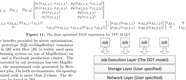
3. BecauseO′J2is a diagonal matrix, considering the rule ofExploiting the Potential of Parallelismin sec-tion 4.4, O′
J2 and TJ2 can be merged into TA1, J1. Thus, A1, J1 and J2 can be represented by a single composite DOT block. An equivalent DOT expression for TPC-H Q17 will only need two composite DOT blocks. This final optimized DOT expression is shown in Figure 11.