Optimal Model-Based Approaches for Predictive Inference in Biology

OPTIMAL MODEL-BASED APPROACHES FOR PREDICTIVE INFERENCE IN BIOLOGY

A Dissertation by

JASON MATTHEW KNIGHT

Submitted to the Office of Graduate and Professional Studies of Texas A&M University

in partial fulfillment of the requirements for the degree of DOCTOR OF PHILOSOPHY

Chair of Committee, Edward Dougherty Co-Chair of Committee, Ivan Ivanov

Committee Members, Jean-Francois Chamberland Head of Department, RobertMiroslav Begovic Chapkin

May 2015

Major Subject: Electrical Engineering

ABSTRACT

Predictive modeling of the dynamic, multivariate, non-linear, stochastic systems of biology is a difficult enterprise. High throughput measurement techniques are enabling new approaches to computational biology, but the small number of sam-ples typically available relative to the number of features measured make additional sources of information critical for accurate predictions. In this dissertation, we offer an approach to incorporate biological pathway knowledge into a predictive stochastic model for genetic regulatory networks. In addition, we propose a statistical model for shotgun sequencing and use computational approximation strategies to derive optimal estimators for classification.

We perform comparisons of classifiers trained using this framework to other ex-isting classification rules including non-linear support vector machines. Using both synthetic and real sequencing data, our classifiers delivered lower classification error rates than existing classification techniques. In addition, we demonstrate using prior knowledge to construct the classifier through properly constructed prior distributions and several scenarios where this increases classification performance.

This research establishes a flexible framework to generate optimal estimators with respect to statistical biological models. By demonstrating the role and power of computation in unlocking these estimators, we point future research efforts towards this computationally intensive approach for the computational biology field.

DEDICATION

ACKNOWLEDGEMENTS

I first would like to thank my parents Bud and Debbie Knight. Without their love and support in all its forms, I would not have had the freedom and courage to be who I am today. I also thank Bryan for his persistent flame of curiosity, Michelle for leading me away from hubris, and my beloved Emily for her enormous support and love in our journey and the patience which she will continue to need for the years to come!

I’d also like to thank my advisors: Ed Dougherty for teaching me to aspire to the higher planes of optimal estimation over ad-hockery and to having a sound epistemology; Ivan Ivanov for teaching me wisdom in navigating the often treacherous landscapes of science; and Robert Chapkin for showing me what first class science looks like and the importance of transparency in all things. I also thank Jean-Francois Chamberland for acting as my committee member and reinforcing rigor in all things. The members of the GSP and Chapkin labs were crucial in raising my standards of quality and productivity, keeping things interesting, and always being there in support, in no particular order I’ll list the most notable: Dr. Laurie Davidson, Jen-nifer Goldsby, Karen Triff, Dr. Tim Hou, Robert Fuentes, Eunjoo Kim, Dr. Roger Zoh, Dr. Manasvi Shah, Jason Xingde Jiang, Dr. Sriram Sridharan, Dr. Mohammad Shahrokh, Dr. Esmaeil Gargari, Dr. Ting Chen, Dr. Chen Zhou, Dr. Youting Sun, Dr. Mohammad Yousefi-Rezaei, Dr. Lori Dalton, Dr. Amin Zollanvari, and Dr. Fang Hsu. And lastly, I thank my friends and workout partners Edwin Eigenbrodt and Edward Talmage for waging war against physiological atrophy and hastening the heat death of the universe.

NOMENCLATURE

Probabilistic State Transition Graph PSTG

OBC BEE

Optimal Bayesian Classifier Bayesian errorestimate

MSEBEE the estimated Mean Square Error of the BayesianError Estimator MCMC Markov chain Monte Carlo

TABLE OF CONTENTS Page ABSTRACT . . . ii DEDICATION . . . iii ACKNOWLEDGEMENTS . . . iv NOMENCLATURE . . . v TABLE OF CONTENTS . . . vi LIST OF FIGURES . . . ix

LIST OF TABLES . . . xiv

1. INTRODUCTION . . . 1

1.1 Contributions . . . 2

1.1.1 Markov models for pathway knowledge . . . 2

1.1.2 Optimal Bayesian classification for non-Gaussian sequencing datasets . . . 4

1.2 Organization . . . 6

2. FROM BIOLOGICAL PATHWAYS TO PREDICTIVE MODELS . . . 7

2.1 Introduction . . . 7

2.2 Obtaining the pathways . . . 9

2.3 Creating Karnaugh maps from pathways . . . 12

2.4 Probabilistic state transition graphs . . . 15

2.5 Simulating long run behavior . . . 19

2.5.1 A synthetic example . . . 19

2.5.2 The general method . . . 21

2.5.3 The steady state activity vector . . . 22

2.6 The NF-κB system . . . 24

2.7 Towards model validation using knockout studies . . . 27

2.7.1 A20−/− _{. . . 28}

2.7.2 IKKβ−/− and TNFR−/− . . . 30

2.7.4 IKKα−/− . . . 31

2.7.5 IKKβ−/− . . . 32

2.7.6 NEMO−/− _{. . . 32}

2.8 Conclusions . . . 33

3. MCMC IMPLEMENTATION OF THE OPTIMAL BAYESIAN CLAS-SIFIER FOR NON-GAUSSIAN MODELS: MODEL-BASED RNA-SEQ CLASSIFICATION . . . 37

3.1 Background . . . 37

3.2 Methods . . . 40

3.2.1 Notation . . . 40

3.2.2 Review of optimal Bayesian classification . . . 40

3.2.3 Conditional error estimator . . . 45

3.2.4 The multivariate Poisson model . . . 46

3.2.5 Overdispersion . . . 49

3.2.6 Prior calibration using discarded features . . . 51

3.2.7 Computation . . . 54

3.2.8 Synthetic data . . . 56

3.2.9 Real data . . . 59

3.3 Results and discussion . . . 60

3.3.1 Synthetic data . . . 60

3.3.2 Real data . . . 63

3.3.3 Computational limitations . . . 65

3.4 Conclusions . . . 66

4. DETECTING MULTIVARIATE GENE INTERACTIONS IN RNA-SEQ DATA USING OPTIMAL BAYESIAN CLASSIFICATION . . . 68

4.1 Introduction . . . 68

4.2 Methods . . . 69

4.2.1 Optimal Bayesian classification . . . 69

4.2.2 Computation . . . 72

4.2.3 Normalization . . . 76

4.2.4 MCMC convergence diagnostics . . . 76

4.3 Dietary intervention study . . . 77

4.4 Results . . . 79

4.4.1 Differential expression analysis . . . 79

4.4.2 Overall error distributions . . . 80

4.4.3 Biological findings . . . 85

4.5 Conclusion . . . 88

REFERENCES . . . 91 APPENDIX A. ADDITIONAL ALGORITHMS FOR OPTIMAL BAYESIAN

CLASSIFICATION . . . 102 APPENDIX B. ADDITIONAL FIGURES FOR OPTIMAL BAYESIAN

CLAS-SIFICATION . . . 106 APPENDIX C. ADDITIONAL BAYESIAN POSTERIOR P-VALUES . . . . 111

LIST OF FIGURES

FIGURE Page

2.1 The process of developing the Karnaugh map using the pathways as-sociated with NEMO. For each step in the process, we evaluate each pathway in turn. In each pathway, the predicate specifies certain lo-cations in the Karnaugh map and these are shaded in yellow in the corresponding table. Reproduced with permission from [56]. . . 13 2.2 A simplified PSTG for the NEMO protein with predictors that are all

static for the purposes of illustration. Here the binary value of the state should be interpreted as [A20, LTβR, RIP1, NEMO]. The red, dashed edges represent one possible configuration of the network, while the blue, dotted edges represent the other configuration. Reproduced with permission from [56]. . . 16 2.3 A synthetic example of the complete process from pathways to long

run probabilities. (A) Pathways for the three proteins: protein A has no predictors, B is predicted by A, and C is predicted by A and C. (B) The resulting Karnaugh maps with one final conflict obtained using the method described in Algorithm 1. (C) The resulting PSTG shows two separate basins. The left basin has a single attractor state 001 while the right basin has two states in the attractor,111 and110. (D-F) The probability mass in each state at the (D) initial stage (E) after the first state transition, and (F) after many state transitions have taken place. (G) The resulting protein B knockout (B= 0) PSTG. The state space is halved as the states with B=1 are no longer considered in the possible transitions. Reproduced with permission from [56]. . . 17

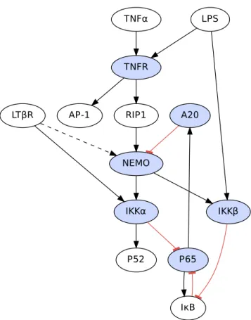
2.4 The resulting communicating class of states for the full NF-κB PSTG when the stimuli conditions are set to TNF=1, LPS=0, and LTβR=0. The thirteen bit binary vector can be read as[A20, AP-1, IκB, IKKα, IKKβ, LPS, LTβR, NEMO, p52, p65, RIP1, TNFα, TNFR]. To give a walk through of one state transition, starting at the upper right state, 0100000010111, many things occur in one transition: IκB is inactive and thus at the next state p65 translocates to the nucleus to become active; NEMO is activated by RIP1; p52 is deactivated as IKKαis not activating it; and IκB becomes active, as constitutive expression allows it to repopulate the cytoplasm in the absence of activated IKKβ. All of these changes results in the model evolving to state 0110000101111. Reproduced with permission from [56]. . . 23 2.5 The pathway structure of the NF-κB system. Blue proteins are those

that are knocked out in the validation portion of this section. The presence of a directed edge indicates that a pathway exists that shows the upstream protein causes a change in the activity of the down-stream protein. Inhibitory pathways are marked red and terminated with a filled dot. One thing to note here is that the LPS induced autocrine production of TNFα would seemingly imply that an excita-tory connection should be made between LPS and TNFα. However, because we want to exogenously control TNFα, LPS, and LTβR in our knockout simulations, we consider TNFαto be an exogenous stimulus, thereby allowing us to control that level in simulations without affect-ing the autocrine feedback loop of LPS. The second thaffect-ing to note is the dotted connection from LTβR to NEMO which indicates this is a pathway with unknown mechanism but described in [43]. Reproduced with permission from [56]. . . 25 3.1 A Bayesian classification derivation tree summarizing the relationships

between several important quantities in the general theoretical frame-work of Bayesian classification. A directed edge between a parent and its child indicates that the child can be derived from the parent by the equations indicated in the edge label. The root of the tree p(θ|Sn) is the posterior distribution of the feature label parameters and by tak-ing expectations with respect to this distribution, we can derive the effective class conditional densities p(x|y, Sn) and the distribution of the classifier errorp(ε|Sn). Then these quantities give rise to the OBC, and MMSE and MSE estimates for the error as described in the text. Quantities highlighted in grey are given in closed form for Gaussian and multinomial distributions in [17]. Reproduced with permission from [57]. . . 42

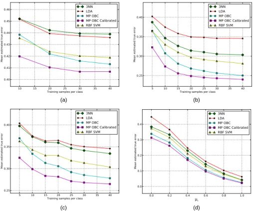
3.2 Mutivariate Poisson model plate diagram. A plate diagram for the multivariate Poisson model. The outermost plate represents the classes that we are interested in classifying against, where i is the index of the sample in classy, and j are the genes being modeled. Reproduced with permission from [57]. . . 48 3.3 Synthetic data classification results with (a) homogeneous-covariance,

(b) high correlation covariance, (c) low correlation independent-covariance, and (d) high correlation independent-covariance data at several problem difficulties. Reproduced with permission from [57]. . 61 3.4 TCGA RNA-Seq Classification. Average holdout errors were

com-puted over 10,000 training sets and feature subsets using two types of lung cancer RNA-Seq data from TCGA. MP OBC with and with-out calibrated priors demonstrates superior performs across a range of training sample sizes. In addition, providing the MP OBC with calibrated priors does not appear to improve performance in this par-ticular dataset. Reproduced with permission from [57]. . . 65 4.1 BEEMSE calculations utilize MCMC sampling from the posterior of

θ. Then for each sample of θ, ε|θ is approximated using a draw of x

fromp(x|y,θ). Then the conditional BEE error is computed for each of these in order to form a Monte Carlo approximation to ε|θ. Then

these approximations are again used in a Monte Carlo integration step to approximate εˆand _E[ε2]. . . 74 4.2 Computation of∆is sensitive to Monte Carlo approximation error so

naive calculations of each error quantity are inadequate. Instead we used the above scheme where the main insight is that the BEE com-putation for each gene subset must be made using the same MCMC samples of θ but projected down to the appropriate dimension. This

results in the∆ quantities shown in Fig. 4.8. . . 75 4.3 Classification of 858 genes from prior knowledge was performed with

an expression filtration step, then BEE calculations were performed on all 1.7M gene sets across the three comparisons and two dimensional-ities (sets of two and three genes). Then the lowest 1000 classification error sets were selected from each comparison and run in additional BEEMSE and ∆calculations. . . 78

4.4 For the fpa-cca comparison the above histogram for all 12,000 genes and for the 858 genes in the prior knowledge gene list show that the majority of genes in the prior knowledge list set are not differentially expressed and have a distribution of P-values to the entire dataset. . 79 4.5 The overall classification error distributions are shown by the

num-ber of features (panel x-axis), dietary comparison (panel y-axis), and normalization type (stacked plot colors). Average classification error is slightly lower (0.28 vs 0.30) as expected for classification with 3 genes when compared against two genes. Additionally, the three di-etary comparisons (oil and fiber types (FP/CC), oil only (FP/CP), and fiber only (CP/CC)), showed differences in average classification performance. . . 81 4.6 For the best 1000 gene sets for each dietary comparison, the BEEMSE

tends to increase as a function of BEE. . . 83 4.7 Normalized count expressions are shown for the three genes Arg2,

Lgals3bp, and Adamts1. The cubes and spheres indicate the fpa and cca samples, respectively. Using the marching cubes contouring al-gorithm, an approximate rendering of the nonlinear OBC decision boundary is also displayed. . . 84 4.8 The distribution of∆for the top 1000 gene sets of the three

compar-ison groups. CPA-CCA has the largest ∆ values which corresponds to that comparison having the largest classification errors. Negative values of ∆ are due to approximation error. . . 85 4.9 Overall classification error varied depending on whether normalization

was used (None) and whether it was implemented as a pre-processing step applied to the data (Counts) or input into the model through the sequencing depth variable d (Model). . . 86 4.10 Normalized counts of the Fabp1 and Eno3 genes were plotted against

each other in relation to the OBC decision boundary (black line) for the fpa-cca comparison. . . 87 B.1 The multivariate normal distribution used to generate samples for

the IC synthetic data case. The block structure indicates the several different types of features that are generated. Used with permission from Ghaffari et al., 2013 [36]. . . 107

B.2 A simple two class, two gene, synthetic example demonstrates the use of the MP OBC. Six training samples from each class (circles and triangles) are shown in all four panels and used to train the MP model. After MCMC computation, the resulting effective class conditional density contour is shown for the triangles in panel a and the circles in panel b. Panel c then shows the resulting MP OBC decision boundary resulting from these effective class conditional densities and panel d shows the contours of the optimal Bayes conditional error estimate plotted next to the classifier decision boundary. Reproduced with permission from [57]. . . 108 B.3 Using the same classifier, we can now evaluate the performance of the

classifier using 3000 testing samples from each class. When evaluated and averaged, this particular example results in a classification error of 0.29. Reproduced with permission from [57]. . . 109 B.4 Two examples of 100 samples from adenocarcinoma TCGA tumor

samples and the posterior predictive xrep simulation from the MP model. Reproduced with permission from [57]. . . 110

LIST OF TABLES

TABLE Page

2.1 Pathways comprising the NF-κB system. Reproduced with permission from [56]. . . 11 2.2 Knockout studies and simulations. Reproduced with permission from

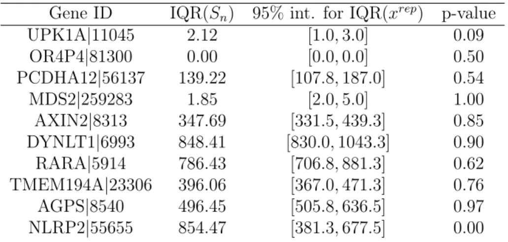
[56]. . . 29 3.1 Posterior predictive model diagnostics are given for 10 randomly

se-lected genes from adenocarcinoma TCGA samples. Inter-quartile dis-tance (IQR) is used as a robust measure of dispersion. In the table, IQR(Sn) is the training data’s IQR, followed by the 95-th credible interval, and the posterior predictive value. In cases where the P-value is close to 0 or 1, the true test statistic’s distance from the 95-th credible interval can be used to determine the magnitude of the mis-fit. Reproduced with permission from [57]. . . 64 4.1 The top ten differentially expressed genes of the 858 gene list by

ad-justed P-value as reported by DESeq in the fpa-cca comparison. . . . 80 4.2 The top four lowest classification error gene sets for each of the three

comparisons and for two and three genes. In addition, the∆value for the three gene comparisons gives the reduction of classification error when adding the third gene to the best performing gene subset of size two. Errors, MSEs, and ∆s below 0.01 are not displayed here due to the larger relative effects of Monte Carlo error at these value ranges. . 82 C.1 Posterior predictive model diagnostic – 5th quantile. Reproduced with

permission from [57]. . . 112 C.2 Posterior predictive model diagnostic – Median. Reproduced with

permission from [57]. . . 113 C.3 Posterior predictive model diagnostic – 95th quantile. Reproduced

C.4 Posterior predictive model diagnostic – IQR. Reproduced with per-mission from [57]. . . 115 C.5 Posterior predictive model diagnostic – Variance. Reproduced with

1. INTRODUCTION

Biological organisms can be considered high-dimensional, non-linear, stochastic, dynamical systems. Each of these attributes increases the difficulty of making pre-dictions about the behavior of these complex machines. Additionally, the known operational mechanisms of biological systems are only partially catalogued adding another level of difficulty to the task. Despite this, disciplines ranging from medicine to synthetic biology drive the need to develop methodologies to make accurate pre-dictions in the face of this difficult and partially understood domain.

Recent developments in the field of high-throughput biological measurement tech-niques – most notably shotgun sequencing – have increased our ability to probe the internal workings of the cell. These techniques produce measurements of the entire transcriptional profile of a cell, or sequence an entire genome. But despite rapidly dropping costs of these techniques, the number of samples obtained is typically much smaller than the number of features measured. This positions the analyses of these dataset squarely in the “small sample” domain where common statistical assumptions such as asymptotics cannot be relied upon.

Despite the difficulty of the domain and the small number of samples available, two facets of the problem, if properly leveraged, can enable forward progress. First, for decades biologists have worked to discover knowledge regarding the mechanistic underpinnings of biology in the form of pathways. These pathways describe known relationships between genes, proteins, RNAs, and other functional elements of the cell. Secondly, with the data and pathway knowledge available, we are typically not immediately interested in a full understanding of the biological system itself. Instead, we would often like to make predictions about some limited aspect of the

system. For example, medical practitioners often want answers to questions such as, “what subtype of cancer is my patient suffering from?” and “which treatment will lead to the best prognosis?”. Similarly biologists ask targeted questions of their experimental datasets such as, “what mechanism is responsible for this observed shift in phenotype?” and “which experiment should I perform next to discover this mechanism?”

Leveraging those two insights, in this dissertation, we propose techniques to utilize biological pathway knowledge to make predictions about biological systems.

1.1 Contributions

The contributions made in this dissertation result from two primary research projects. First, we developed an algorithm to use biological pathways to construct a stochastic dynamical model for gene regulatory networks. This model can then be used for making predictions of system behavior under unobserved operating con-ditions. We then applied this technique to build an NF-κB regulatory model using pathways from the literature. We then used additional mouse knockout experiments available in the literature for an external qualitative validation. Secondly, we wished to improve this technique to develop an optimal estimation methodology for the in-corporation of prior knowledge with high-throughput data. We achieved this in the realm of classification using Optimal Bayesian Classification and the application of computational approximation techniques.

1.1.1 Markov models for pathway knowledge

The cell is the essential functional unit of life, and an understanding of its internal mechanisms has occupied a large proportion of the productive output of biology. Biological pathways represent a formalization of much of this knowledge in the form of mechanistic dependencies between the functional elements in a cell.

Unfortunately, the information inherent in these pathways is incomplete and often conflicting due to cellular context including epigenetics and internal or environmental conditions for the cell. Additionally, the information is univariate and therefore does not typically provide enough information alone to make accurate predictions in light of the cellular context.

We address that problem in Section 2 by developing an algorithm which takes as an input a set of pathways and outputs a Markov chain model of the system which evolves consistently with the pathways. This requires a procedure to deal with inconsistencies in the pathway information that may arise due to differing cellular context when the pathway was originally discovered.

We then use this Markov chain to make predictions regarding the steady state distribution of the gene/protein expression. These steady state distributions can then be used to predict phenotypes based on known gene actions in the cell.

The NF-κB network is of prime interest in translational medicine and biology as it acts as a hub network of the cellular inflammatory response mechanism. Chronic inflammation is linked to many diseases such as autoimmune disorders, the progres-sion of cancer, and heart disease. Therefore, it is of great interest in translational medicine to produce accurate predictions about the activation of NF-κB given a set of conditions (or treatments) surrounding the upstream signaling network.

We obtained 28 pathways from the NF-κB literature and transformed them into a binary vector valued Markov chain model of the NF-κB network. We then compared the predictions of this Markov chain under seven network perturbations to the litera-ture where a seven analogous mice knockout models were performed. This qualitative validation of the network model demonstrates that pathways can encode enough in-formation regarding the system when intelligently combined, and the Markov chain model maintains this information in a consistent manner enabling predictions under

perturbation which match biological observations under similar perturbations. 1.1.2 Optimal Bayesian classification for non-Gaussian sequencing datasets While the approach taken in Section 2 was seen to produce acceptable predictions, it still remains essentially heuristic. In Section 3, by adopting a cost function and an optimization approach, we find optimal estimators for predictions of biological sys-tems. Specifically, we consider the prediction problem of classification. In addition, instead of considering pathway information, we utilize a new statistical model (this time of the data generation process) in order to operate on labeled sample data and prior distributions to train an optimal classifier.

This work builds on previous work by Dalton and Dougherty [15, 16, 17, 18] where they discovered MMSE classifiers for Gaussian and multinomial distributions. However, we wished to apply these methodologies to sequencing data which is a widespread biological measurement technique and does not conform to Gaussian dis-tributional assumptions. This required a statistical feature-label distribution with considerably more complexity than multivariate Gaussian or multinomial distribu-tions alone. We therefore proposed a hierarchical Poisson model to encapsulate the known processes that sequencing data undergoes from the biology to the resulting measurements.

Utilizing a statistical model that aligns closely with the underlying measurement process provides several advantages over simpler phenomenological statistical models: • Placing prior distributions over the parameters of the model is more straight-forward as the parameters of the model relate to measurable, real world, quan-tities.

• The inferred parameters of the model are easier to interpret and troubleshoot should problems arise.

• The flexible construction of the model allows the addition or subtraction of complexity as the data warrant (or require) it.

The downsides to these complex models is the loss of analytical tractability. We therefore developed a computational approximation strategy to arrive at the op-timal estimators using tools such as Markov chain Monte Carlo and Monte Carlo integration.

We validated the performance of these models and subsequent optimal classifiers on a variety of synthetic datasets against other classification techniques. We also used a real dataset from The Cancer Genome Atlas to classify subtypes of lung cancer sequencing data using the same set of available classifiers. The optimal classifier exhibited superior performance in nearly all cases.

We also applied the same statistical model in a feature selection study to detect groups of genes which well separate phenotypes of interest. In this capacity, we utilized two additional optimal estimators surrounding the prediction problem: the Bayesian error estimate, and the mean square error of the Bayesian error estimate. These two estimates give a salient measure of the separation of the phenotypes and a quantification of the uncertainty in that estimate.

We then applied the three estimators (including the optimal classifier itself) to a dietary animal model dataset to discover gene pairs and triplets that were not individually differentially expressed, but together well separated the groups with low error estimates and low uncertainties around those estimates. This led to novel biological insights to the system which were not available using widely available to the differential expression analysis techniques common in sequencing data analysis.

1.2 Organization

Section 2 introduces a novel algorithm to produce binary vector valued Markov chain models of genetic regulatory networks consistent with biological pathway knowl-edge. Section 3 explains an optimal estimation framework to use prior knowledge and data for sample classification. Section 4 extends the work in Section 3 for feature selection of sequencing datasets using an additional pair of optimal estimators. And Section 5 concludes the dissertation with summarizing remarks and future work.

2. FROM BIOLOGICAL PATHWAYS TO PREDICTIVE MODELS∗

2.1 Introduction

Biological regulatory network models offer the promise of one day applying sys-tems based approaches for cancer diagnosis and therapy [27, 21]. Consequently, it is not surprising that the systems biology literature contains many algorithms to infer such regulatory networks from (time-course) microarray data [46, 72, 24, 1, 45]. Inferring such networks is inherently difficult because of the limited availability of the data and the fact that most of these algorithms do not include mechanisms for incorporating prior knowledge, which could potentially reduce the data requirement. Consequently, most of these network models have not been validated, thereby hin-dering their use in translational science and medicine.

Before the advent of high throughput measurement techniques such as microar-rays and shotgun sequencing, biological experimentation often focused on uncovering (mostly univariate) relationships between genes and proteins in the production of what is usually referred to as pathway knowledge. This pathway knowledge is based on empirical observations across different experiments that have acquired some degree of validity through the peer review process. While not all pathways in the literature are accurate, and some pathways may in fact be conflicting, we believe that they offer an excellent foundation for the network construction process especially when combined with high throughput data for model refinement and validation.

In the absence of any pathway knowledge, one would have to assume that each protein behaves randomly. In other words, with no knowledge of the interactions

∗_{Parts of this section are reproduced with permission from Knight, J.M.; Datta, A.; Dougherty,}

E.R. "Generating Stochastic Gene Regulatory Networks Consistent with Pathway Information and Steady-State Behavior", IEEE/ACM Transactions on Computational Biology and Bioinformatics, 59(6), 1701-1710 2012. doi:10.1109/TBME.2012.2192117 Copyright © 2012 IEEE.

between proteins we cannot predict if a certain protein will be expressed more or less than average over the long run. With available pathway information, however, one can refine the random model by using the knowledge to guide the behavior of the model when the contextual information of the pathway is satisfied. By requiring the model to obey the pathway information, we can be sure that the model reflects the pathway knowledge that is available. By using a significant amount of pathway information we can reduce the data requirement and generate models that produce predictions that are more meaningful than those with little or no prior information. Based on the preceding discussion, it is clear that the long run behavior of the model is a function of the amount of pathway information available about the system and the initial conditions. If we know too little about the system, then the long run behavior will reflect the unknown, random evolution and no conclusions can be made. However, if the long run behavior differs from the stochastic background level, then the pathway knowledge and initial conditions are sufficient to make qualitative predictions about that system. This is what we will be demonstrating in this section by using a model which captures the behavior of the pathways relating to the NF-κB system.

A few key assumptions underlie our model development. The first is the dis-crete state and disdis-crete time approximation of protein behavior. This is a large assumption, but the most important one utilized in this section. It has been vali-dated in many biological contexts [53, 22], and provides an important simplification that enables large scale network modeling with pathway data. Indeed, as pointed out in [63], such discrete-time discrete-state modeling avoids the need for making continuous-time measurements of protein concentrations and facilitates the accom-modation of genes/proteins which exhibit ON/OFF switch-like behavior. Moreover, discrete time systems are easier to analyze, model and control in real time [60].

The second assumption that we make is that there is no prior knowledge about the initial state of the cell and only the presence or absence of external stimuli is known. In other words, we assign a uniform initial distribution to all possible states and allow the pathway constrained model to stabilize into attractor cycles. This assumption has the effect of distributing the resulting probability mass of the cell states to the states that are in the attractor cycles. Furthermore, these attractor cycles have a total probability that is proportional to the size of the basin of attraction. A similar conclusion was reached by Huang [49] but from a biological argument of cellular homeostasis in the presence of continual perturbations of the inter and intra cellular environments.

In this section, we propose a new method for generating networks from pathway information. We then apply this method to the set of proteins that compose the NF-κB regulatory network to build the transition probability matrix of a discrete-state, discrete-time Markov chain that produces predictions that agree with the literature. The NF-κB system was chosen due to the prevalence of associated pathway infor-mation in the literature as well as due to its biological importance in cancer and the innate immune system.

2.2 Obtaining the pathways

In any network inference procedure, the first step consists of selecting a specific biological system and choosing the specific agents for inclusion in the model. In this section, this task was performed manually, although future work could include using selection techniques such as statistical tests on high-throughput data to identify the most relevant molecules for state based modeling.

The model generated in this section consists of protein species with the exception of one lipoglycan (lipopolysaccharide). In general, the species in the pathways and

the resulting model can be a mixture of any types of biological entities as long as the pathways are accurately reflect the relationships being studied. Throughout this section, we will refer to the elements in the model as proteins with the tacit understanding that sometimes other biological entities would also be admissible.

To obtain pathway data for this section, we manually reviewed the biological literature relevant to the NF-κB system and recorded a pathway when significant biological evidence was available and the molecules involved in the pathway were chosen to be significant. For interactions that included non-significant species, the pathway was either ignored or extended upstream and downstream until it included significant species. The resulting pathways and the references used to arrive at them are summarized in Table 2.1. A full description of the NF-κB system appears later in section 2.6.

Here each pathway description consists of two parts, the predicate and the subject and are separated by the implication sign, =⇒. The information that the pathway

contains can be understood as: “when the predicate is true, the subject is implied to occur in the future." The timing with which this dependence occurs is not known, but in this section we assume that the dependence relationship is implemented at the next time step as in [63].

Using the pathway data, one can determine which proteins are upstream of each other and also determine the set of predictor proteins, i.e. the proteins whose ac-tivity status collectively determines the time course updates of a given protein. In the general case, it is possible that one could have this information without having any pathway knowledge about the specific behavior of the regulation. While the algorithm presented below can handle this case equally well, in the NF-κB model considered here we did not have any knowledge of this type and therefore the pre-dictor sets were derived directly from the pathway knowledge.

Table 2.1: Pathways comprising the NF-κB system. Reproduced with permission from [56]. Pathway Reference RIP1= 1 =⇒ NEMO= 1 [43] A20= 1 =⇒ NEMO= 0 [43] LTβR= 1 =⇒ NEMO= 1 [43]

A20= 1 and RIP1 = 1 =⇒ NEMO= 0 [43] RIP1= 0 and LTβR= 0 =⇒ NEMO= 0 [43]

TNFR= 1 =⇒ AP-1= 1 [43] TNFR= 0 =⇒ AP-1= 0 [43] TNFR= 1 =⇒ RIP1= 1 [44] TNFR= 0 =⇒ RIP1= 0 [44] LPS= 1 =⇒ TNFR= 1 [54] TNFα= 1 =⇒ TNFR= 1 [54] LPS= 0 and TNFα= 0 =⇒ TNFR= 0 [54] IKKα= 1 =⇒ p52 = 1 [43] IKKα= 0 =⇒ p52 = 0 [43] LTβR= 1 =⇒ IKKα= 1 [43] NEMO= 1 =⇒ IKKα= 1 [43]

NEMO= 0 and LTβR= 0 =⇒ IKKα = 0 [43]

NEMO= 1 =⇒ IKKβ = 1 [90]

LPS= 1 =⇒ IKKβ = 1 [44]

NEMO= 0 and LPS= 0 =⇒ IKKβ = 0 [90, 44]

p65= 1 =⇒ IκB = 1 [43, 88] p65= 1 =⇒ A20= 1 [43, 88] p65= 0 =⇒ A20= 0 [43, 88] IKKβ = 0 =⇒ IκB = 1 [43] IKKβ = 1 =⇒ IκB = 1 [43] IκB= 1 =⇒ p65 = 0 [43] IκB= 0 =⇒ p65 = 1 [43] IKKα= 1 =⇒ p65 = 0 [61]

Let us now demonstrate this algorithm on a part of the NF-κB system. From Table 2.1, we consider the pathways related to the behavior of NEMO. These are the first five entries in that table and are given by:

RIP1= 1 =⇒ NEMO= 1 (2.1) A20= 1 =⇒ NEMO= 0 (2.2) LTβR= 1 =⇒ NEMO= 1 (2.3) A20= 1 and RIP1 = 1 =⇒ NEMO= 0 (2.4) RIP1= 0 and LTβR= 0 =⇒ NEMO= 0 (2.5)

The pathways listed above mandate the following relationships: when RIP1 is activated, it activates NEMO; when A20 is activated, it deactivates NEMO; when LTβR is activated, it activates NEMO; when both A20 and RIP1 are activated, NEMO is deactivated; and when RIP1 and LTβR are both inactive, NEMO is de-activated. From these, we can infer that a reasonable predictor set for NEMO is

{A20,LTβR,RIP1}. One can similarly arrive at predictor sets for the other

biologi-cal entities in Table 2.1.

2.3 Creating Karnaugh maps from pathways

Having identified the predictor set for each protein, we can use a Karnaugh map [52] to determine the update rule for that protein. The method used is an extension of the one developed in [63]. For each protein, using its predictor set, we initialize a Karnaugh map with every entry in the map containing the unknown ‘x’. This is consistent with the observation that to start with we have no information about how the current value of the prediction proteins affects the update value of the predicted

x RIP1 A2 0, L T βR 0 1 01 00 x x x NEMOnext 11 10 x x x x A 11 RIP1 A2 0, L T βR 0 1 01 00 x 11 11 NEMOnext 11 10 c1 c₁ 0₁ c1 D x RIP1 A2 0, L T βR 0 1 01 00 x 11 11 NEMOnext 11 10 x 11 x 1₁ B 11 RIP1 A2 0, L T βR 0 1 01 00 x 11 11 NEMOnext 11 10 c1 0₂ 0₁ 02 E x RIP1 A2 0, L T βR 0 1 01 00 x 11 1₁ NEMOnext 11 10 0₁ c1 01 C c1 11 RIP1 A2 0, L T βR 0 1 01 00 02 11 11 NEMOnext 11 10 c1 02 0₂ F 0₂

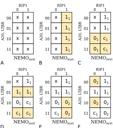
Figure 2.1: The process of developing the Karnaugh map using the pathways asso-ciated with NEMO. For each step in the process, we evaluate each pathway in turn. In each pathway, the predicate specifies certain locations in the Karnaugh map and these are shaded in yellow in the corresponding table. Reproduced with permission from [56].

protein at the next time step. The Karnaugh map entries can then be updated by incorporating the pathway information. For instance, consider the update of NEMO. The initial blank Karnaugh map for it is shown in Fig. 2.1A. We will refer to the locations in the Karnaugh map using the vector [A20, LTβR, RIP1]. Thus000would correspond to the square in the upper left corner of the map and so on. Now, using the first pathway: RIP1 = 1 =⇒ NEMO = 1, we can fill all the entries that correspond to RIP1=1 with ones, and this results in the Karnaugh map shown in Fig. 2.1B.

We next proceed to fill the locations 100 and 110 with zeros to satisfy the re-quirements of the second pathway: A20 = 1 =⇒ NEMO= 0, but are faced with a conflict when RIP1=1 and A20=1. At the two conflicting locations we replace the ones with c1. The letter c indicates a conflict while the superscript 1 indicates that

the conflict comes from pathways which contain only one protein in the predicate. The reasoning for this notation will become clear later in this section. This results in the table in Fig. 2.1C.

We next consider pathway three: LTβR= 1 =⇒ NEMO = 1, which mandates that the ’x’ at location 010be replaced by a 1. Since location110contains a 0, so we replace it with a c1 _{to indicate that there is a conflict. Finally, location111 already}

has a c1and because this pathway only contains one protein in its predicate, we must

leave the c1 in place. This leads to the table shown in Fig. 2.1D.

Next we look at the fourth pathway: A20= 1 and RIP1 = 1 =⇒ NEMO = 0. The predicate here applies to locations101and111. Both of these contain c1conflicts, but because this pathway contains two proteins in its predicate, we acknowledge this pathway has more specific information regarding this particular experimental scenario and can override the c1 _{conflicts. Therefore we fill the locations101and111}

For the final pathway: RIP1= 0 and LTβR= 0 =⇒ NEMO= 0, the predicate applies to the locations 000and 100. The former has an x, so we replace it with a 0, and the latter is already a 0. Therefore we are now finished with NEMO’s pathway information and are left with the Karnaugh map of Fig. 2.1F. In this map, we see there is only one uncertainty condition at the location 110.

The procedure demonstrated on the NEMO example above can be generalized by proceeding through the pathways in order from the least specific predicates to the most specific ones and filling in the Karnaugh map entries if information is available or invalidating information already provided if there are conflicts in the pathway information. This general procedure is presented in Algorithm 1. The key difference between the algorithm presented in [63] and the one presented here is that in [63], one attempts to resolve the conflicting entries in the Karnaugh maps by suitably altering the timings of some of the pathways whereas here the conflicts in the Karnaugh maps are retained. Consequently, the state transitions following a conflict will not be unique and by assuming that all the subsequent states are equiprobable, we can come up with probabilistic state transition graphs which are introduced next.

2.4 Probabilistic state transition graphs

The Karnaugh maps generated using the procedure of the last section can be used to produce the probabilistic state transition graph (PSTG) of the system. A PSTG is a directed graph that describes the evolution of the biological system through time. It consists of kn nodes that correspond to the states of the system where k is the number of quantization levels associated with the activity state of each protein (assumed throughout the rest of this section to be two for a binary discretization) and n is the number of proteins in the system. Additionally, each directed edge indicates a viable transition between states as allowed by the pathway information.

0000 0001 0010 0011 0100 0101 0110 0111 1000 1001 1010 1011 1100 1101 1110 1111

Figure 2.2: A simplified PSTG for the NEMO protein with predictors that are all static for the purposes of illustration. Here the binary value of the state should be interpreted as [A20, LTβR, RIP1, NEMO]. The red, dashed edges represent one possible configuration of the network, while the blue, dotted edges represent the other configuration. Reproduced with permission from [56].

For example, using the NEMO pathways and the Karnaugh map generated in the last section we obtain a simplified but illustrative example of a PSTG for this system as shown in Fig. 2.2. We assume here that the predictor proteins have no predictors themselves and therefore exhibit static behavior. This is seen in Fig. 2.2 where the edges of the PSTG, or the allowed transitions, are between states with identical values for the predictor proteins and only differing in the values of NEMO. Also, based on the Karnaugh map generated from the NEMO pathways, we expect uncertainty at the state 110x and indeed, both the states 1100 and 1101 have two outgoing edges each. One of these creates a self loop, and the other directs to the corresponding state with the value of NEMO flipped.

The PSTG is actually a compact representation for the class of networks which the uncertain Karnaugh maps such as the one in Fig. 2.1F generate. To use the example above, we could also represent the uncertainty of NEMO at 110x by creating two separate networks with two corresponding state transition diagrams. One network would contain the blue, dotted edges in Fig. 2.2 and predict that NEMO should equal 0 when A20=1, LTβR=1, and RIP1=0, while the other would have the red, dashed edges and predict that NEMO should equal one for the same set of predictor values.

Bnext A 0 1 1 0 Cnext 0 A B 0 1 1 0 1 1 c1 C A B A = 1 ⇒ B = 1 A = 0 ⇒ B = 0 A = 1 ⇒ C = 1 B = 1 ⇒ C = 0 A = 0 and B = 0 ⇒ C = 1 F D E 000 001 010 011 100 111 101 110 0.125 0.125 0.125 0.125 0.125 0.125 0.125 0.125 0.25 0.25 0.0 0.0 0.0 0.375 0.0 0.125 0.0 0.5 0.0 0.0 0.0 0.25 0.0 0.25

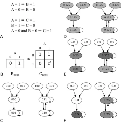
Figure 2.3: A synthetic example of the complete process from pathways to long run probabilities. (A) Pathways for the three proteins: protein A has no predictors, B is predicted by A, and C is predicted by A and C. (B) The resulting Karnaugh maps with one final conflict obtained using the method described in Algorithm 1. (C) The resulting PSTG shows two separate basins. The left basin has a single attractor state 001 while the right basin has two states in the attractor, 111 and 110. (D-F) The probability mass in each state at the (D) initial stage (E) after the first state transition, and (F) after many state transitions have taken place. (G) The resulting protein B knockout (B= 0) PSTG. The state space is halved as the states with B=1 are no longer considered in the possible transitions. Reproduced with permission from [56].

Let us now demonstrate the process of converting Karnaugh maps to PSTGs. We will use the synthetic example in Fig. 2.3A where we are given five pathways for the three proteins A, B, and C. These produce the two Karnaugh maps in Fig. 2.3B and the resulting PSTG is shown in Fig. 2.3C. As can be seen, protein A has no predictors and thus the state space can be partitioned into two basins according to its activity.

To produce the PSTG in Fig. 2.3C, we begin by listing all the possible23 states as unconnected nodes in a graph. Then, for each node we use the Karnaugh maps to update the status of each gene and then concatenate this information to determine the next state to which the model will transition to. For example, for the state 000, protein A has no predictors and therefore no Karnaugh map so we assume it remains in the state 0. Using protein B’s Karnaugh map, A is currently 0, so Bnext = 0. Finally, proteins A and B being zero imply Cnext = 1. Combining all this

information creates a transition edge from state 000 to 001 in the PSTG.

As another example, consider the state111. Following the above logic, Anext = 1

and Bnext = 1 but Cnext is a conflict, so 111 will progress to 11x which can be

expanded to 110 and 111. This is shown in Fig. 2.3C, where the node 111 has two outgoing edges, a self loop and an edge linking to 110.

The PSTG, as in Fig. 2.3C, can also be interpreted as the state transition graph of a Markov chain. Thus, the Karnaugh maps can be converted into a 2n × 2n (n= 3 here) transition probability matrix where each entry[pi,j]2n_×2n represents the probability of the model transitioning from state i to statej in one time step. This matrix is stochastic, and is a row normalized sum of the individual deterministic state transition matrices of the resulting class of Boolean networks that would be required to accommodate the uncertainties associated with the different Karnaugh maps. The PSTG is a compact, sparse representation of this transition probability

matrix, and this is what motivates us to use this framework to simulate the long run behavior of the model.

2.5 Simulating long run behavior

A chief objective of the developed model is to obtain some useful measure of the long run behavior of the system akin to the steady state distribution for an ergodic Markov chain. Unfortunately, the PSTG generated using the above method does not necessarily provide an irreducible or aperiodic state space. Therefore, we must approximate its long run behavior as explained in the following subsections.

2.5.1 A synthetic example

For illustrative purposes we start with the synthetic example in Fig. 2.3. Since we do not have any prior knowledge as to whether a given cell exhibits activated protein A, we make no assumptions about the cell initially being in either basin. In general this would apply to all the proteins in our model and ,therefore, we initialize the states in our network with uniform initial probabilities of0.125 each as shown in Fig. 2.3D.

We can think of this initial probability as our initial belief of the state of the system. Then the algorithm can be understood as an application of the knowledge incorporated in our model to refine the initial belief. We will refer to this belief as the probability mass.

For transitions between states we again utilize uniformity by assuming that the transition probability from one state to the chronologically next one is equal to the inverse of the outgoing degree from the state of origin. So for a state with two outgoing edges such as 110 in Fig. 2.3C, the probability to transition to any of its children (110 and 111) will be 0.5.

progress in one time step to state 000, so we can move the probability mass in state 010 to state000. The same applies to state011 as its mass will “flow" to state 000. Now, state 110 has two outgoing edges, so our model is ambiguous about whether a cell in state 110 will stay in state 110 or if it will transition to 111. Therefore, we split the probability mass in state 110 and place half of it in state 110 and half in state 111 for the next time step. The result of the first run of the process is seen in Fig. 2.3E.

Through iteration of this process, the probability in each transient state tends towards0.0. This can be seen in the example as after the first step of the algorithm, the states along the top are transient because once we leave them, we never return. This is clear from Fig. 2.3E where the probability mass has already been depleted from these transient states and will remain at 0.0 for the remaining lifetime of the model under these conditions. At the next stage, we arrive at Fig. 2.3F, from which we can see that after the second iteration of the algorithm, state000has no remaining probability mass and will remain that way for the remaining simulation because the state is transient and has no return path.

In simple attractor cycles such as the one consisting of the nodes111 and 110 or singleton attractors such as001in Fig. 2.3F, we can calculate the long run probability mass intuitively. The resulting mass in a singleton attractor is obtained by summing all the initial masses in its basin of attraction. For simple attractor cycles, we can sum all of the initial mass in the basin of attraction for that cycle and divide it by the number of nodes in the cycle. In this way, we can get an approximation about how often we could expect the biological system to exist in certain states.

2.5.2 The general method

The intuitive reasoning described above where we iterate over the nodes and add their masses to the downstream nodes applies when the PSTG is acyclic and a preorder traversal through the graph exists. However, with the possibility of cycles, no such preorder traversal must exist and we are forced to introduce an accumulation buffer to describe a general algorithm that works with cycles for any node traversal order.

Let each node have a probability mass and an accumulation buffer. For each node we first initialize the mass of each node to be uniformly distributed over the entire graph, and set the accumulation buffer to zero. Then for each node divide its current probability mass by the number of its outgoing edges and then add that amount to the temporary accumulation buffers for each of its child nodes. Then for each node, set the probability mass to be the value in its accumulation buffer and reset the accumulation buffer to zero.

Repeating this algorithm will result in the probability mass accumulating in the attractors of the system. In the case of aperiodic attractors, the masses will converge to a limiting probability mass, but we must be careful about handling the possibility of periodic attractors. Repeatedly using the algorithm in this case might result in the propagation of an unbalanced mass around the cycle, analogous to oscillatory behavior in undamped systems. To overcome this problem, it is necessary to first run the algorithm a sufficient number of times to eliminate all the transient states and then go through several runs of the algorithm and the final probability mass in the attractor cycle states can then be taken to be an average of the probability masses from the final runs. This essentially smoothens out any oscillations in the probability mass distribution in the attractor cycles.

2.5.3 The steady state activity vector

Now, from a biological point of view, it is more relevant to determine how often a particular protein is active instead of determining how much time is spent in a particular state. Accordingly, we apply a transformation to the long run probability approximation, and define a steady state activity (SSA) vector with n components, indexed by 0 to n−1, corresponding to the n proteins in the model. The i-th com-ponent of the SSA vector, characterizing the activity of thei-th protein, is computed as: SSA(i) = 2n₋₁ X j=0 PA(j)zi(j)

where zi(j) is the binary value of the i-th protein in the j-th decimal state, and PA(j) is the j-th entry of the Probability Approximation vector resulting from the algorithm presented in the previous subsection. The resulting SSA(i) takes values in the interval [0,1] according to the probability that the model is likely to exist in states where proteini is active. For example, an SSA(i)value of1indicates that the i-th protein is active in every attractor state.

Applying this to our example, in Fig. 2.3F, the SSA for protein A, i.e. SSA(0), is calculated by considering the two attractor states111 and110 with active protein A as shown in the right hand basin in the figure. Therefore,SSA(0) = 0.25+0.25 = 0.5. Similarly, SSA(1) (B) is also0.5while SSA(2) (C) is0.75, the latter being due to the fact that all attractors have protein C active except the state 110 which has a final mass of 0.25.

We next further justify the need for using the SSA vector instead of the state vector. Consider the network that we have constructed by applying Algorithm 1 to the set of 28 pathways involving NF-κB. With the external stimuli set to TNFα = 1,

0100000010111 0110000101111 0100000011111 1110000101111 0100000110111 0111100101111 0100000111111 1111100101111 0101100010111 0101100011111 1100000110111 1100000111111 1110000110111 1110000111111 0101100110111 0101100111111 1101100110111 1101100111111 1111100110111 1111100111111 0110000000111 0110000100111 0110000001111 1110000100111 0111100100111 1111100100111 0111100000111 0111100001111 1100000010111 1100000011111 1110000001111 1111100001111 1101100010111 1101100011111 1110000010111 1110000011111 1111100010111 1111100011111 1110000000111 1111100000111

Figure 2.4: The resulting communicating class of states for the full NF-κB PSTG when the stimuli conditions are set to TNF=1, LPS=0, and LTβR=0. The thirteen bit binary vector can be read as[A20, AP-1, IκB, IKKα, IKKβ, LPS, LTβR, NEMO, p52, p65, RIP1, TNFα, TNFR]. To give a walk through of one state transition, starting at the upper right state, 0100000010111, many things occur in one transition: IκB is inactive and thus at the next state p65 translocates to the nucleus to become active; NEMO is activated by RIP1; p52 is deactivated as IKKα is not activating it; and IκB becomes active, as constitutive expression allows it to repopulate the cytoplasm in the absence of activated IKKβ. All of these changes results in the model evolving to state 0110000101111. Reproduced with permission from [56].

LPS= 0, and LTβR= 0, the only communicating set of states for the resulting PSTG is displayed in Fig. 2.4. Due to the size and complexity of the resulting set of states, it would be difficult, if not impossible, to compare the behavior of this PSTG with that obtained from any of the knockout experiments. The concept of the SSA vector was introduced precisely to ameliorate this problem and aids in carrying out qualitative comparisons with the experimental data. This will be demonstrated in the next section.

2.6 The NF-κB system

Nuclear factor-κB (NF-κB) is a protein dimer from the rel family of transcription factors that promote the expression of over 100 genes, primarily in the immune system [37]. The NF-κB system’s primary role in the immune system is in the production of inflammatory cytokines, small signaling proteins used extensively in cell to cell communication. NF-κB also has both proapoptotic and antiapoptotic effects on the cell and the balance of these responses can be adjusted by the stimulus context.

The NF-κB transcription factor is a key element in the inflammation stress re-sponse pathway. The general architecture of this system is typical of several stress response pathways [84]. The transcription factor NF-κB is sequestered in the cytosol by the “sensor" which in this case is IκB and when degraded by the “transducer" of IKKβ, it allows for a rapid downstream response without the lag associated with de novo protein synthesis. As discussed in [84], this combination of a transducer, sensor, and transcription factor is a common motif seen in stress response pathways and forms the backbone of the NF-κB system.

The mammalian NF-κB family consists of p65 (RelA), RelB, c-Rel, NF-κB1 (p52/p100), and NF-κB2 (p50/p105). NF-κB is constitutively expressed, but se-questered in the cytosol by a family of IκB inhibitor proteins which include the p100

Figure 2.5: The pathway structure of the NF-κB system. Blue proteins are those that are knocked out in the validation portion of this section. The presence of a directed edge indicates that a pathway exists that shows the upstream protein causes a change in the activity of the downstream protein. Inhibitory pathways are marked red and terminated with a filled dot. One thing to note here is that the LPS induced autocrine production of TNFα would seemingly imply that an excitatory connection should be made between LPS and TNFα. However, because we want to exogenously control TNFα, LPS, and LTβR in our knockout simulations, we consider TNFα to be an exogenous stimulus, thereby allowing us to control that level in simulations without affecting the autocrine feedback loop of LPS. The second thing to note is the dotted connection from LTβR to NEMO which indicates this is a pathway with unknown mechanism but described in [43]. Reproduced with permission from [56].

and p105 precursors to p52 and p50, respectively, along with IκBα, IκBβ, IκB, IκBγ, and BCL-3 [43]. These IκBs prevent the NF-κB dimers from reaching their binding sites in the nucleus.

The IκB kinase complex (IKK) consists of the IKKα, IKKβ, and IKKγ (NEMO) subunits. The NEMO (NF-κB essential modulator) subunit is a regulator and main-tains the IKKα and IKKβ subunits in inactive states.

The signaling pathways involved in the NF-κB system are shown in Fig. 2.5. NF-κB activation is generally considered to occur through two separate cascade pathways. The canonical pathway is primarily activated by the proinflammatory cytokine Tumor Necrosis Factor-α (TNFα). When TNFα binds to TNF receptor protein (TNFR), it begins a signaling cascade that through the receptor interacting protein 1 (RIP1) activates the NEMO subunit of IKK which activates both the IKKα and IKKβ subunits [81]. The IKKβ subunit then proceeds to phosphorylate IκB proteins which leads to their destruction through polyubiquitination and allows NF-κB dimers, primarily p65 heterodimers and homodimers to translocate to the nucleus and bind to promoter regions [43].

Bacterial lipopolysaccharide (LPS) is a component of bacterial cell walls that provides an activating stimulus for Toll-like receptors 2 and 4 (TLR2 and TLR4). These receptors also activate the canonical pathway but through MyD88 and Trif intermediary proteins [11] that directly activate the IKKβsubunit without activating NEMO [81]. Also, the LPS dependent pathway indirectly activates the canonical pathway through autocrine stimulation through the production of TNFα.

The alternative pathway is activated through CD40 and LTβR and through the NIK protein directly activates the IKKα subunit which through phosphorylation, processes p100 into p52 which activates the nuclear localization segment (NLS) which allows the p52 dimer to translocate into the nucleus. The alternative pathway also

activates the canonical pathway through an unknown mechanism [43].

NF-κB activates two genes in particular that produce IκB and A20. Both of these act as negative feedback to dampen the response of the canonical pathway. A20 binds to NEMO and impairs the activation of the IKKβ and IKKαsubunits by RIP1 [90]. Additionally, NF-κB activates antiapoptotic genes such as cFLIP (not shown in Fig. 2.5) that counteracts the TNFαinduced activation of the proapoptotic AP-1 family such as c-Jun [76]. Consequently, NF-κB knockouts are likely to exhibit apoptotic behavior when subjected to TNFα stimulation. This will be borne out by some of the knockout studies considered later in the next section.

2.7 Towards model validation using knockout studies

The model developed by us in this section was designed to preserve the biological state transitions and stable state attractor cycles. Accordingly, it seems reasonable to validate our model using the experimentally observed long run behavior of biological systems. We will specifically focus on animal knockout models. This kind of model validation is appropriate given that a long term goal of our research is to enhance medical treatment in patients. Currently, treatment is provided through therapeutic drugs which have physiological effects on the order of 8 to 24 hours which can be considered to be long run behavior in the context of regulatory networks. Thus, long run behavior would be particularly appropriate for predicting drug effects and patient outcomes.

Biologists use knockout models to disable a specific gene or a set of genes in a model animal and then observe the resulting physiology to determine protein functions and interactions. Our stochastic state models also provide us a platform with which we can replicate these experiments and examine the resulting steady states. Comparison of the proteins’ known functions and physiological phenotypes,

the resulting increases or decreases in prevalence, and the recorded physiology of the real knockout experiment together provide us with a mechanism for validating our stochastic state space model. For instance, consider the knockout experiment in Fig. 2.3G. Here we have knocked out protein B. This results in a PSTG where all states with protein B active are no longer considered valid and the resulting model has a PSTG consisting only of states with inactive protein B. This results in two attractor states, one for each original basin.

The PSTG resulting from the 28 NF-κB pathways in Table 2.1 was too large to be visually interpreted, although for illustrative purposes a small subset of it is included in Fig. 2.4. We compared the behavior of our model in a steady state fashion with the phenotypes and measured protein quantities as found in the knockout studies. Due to the qualitative nature of the data collected in the knockout experimental studies used, the comparisons between the model and the study will by necessity be qualitative. We believe that this still allows for satisfactory validation given the complexity of the model, the inherently noisy nature of biological systems and experimentation, and the large number of knockout studies examined.

2.7.1 A20−/−

Werner et al. [88] aimed to derive ordinary differential equation (ODE) models of NF-κB regulation in response to TNFα and LPS stimulation. One of their model parameters includes the negative feedback of A20, and to justify this, they compared A20+/+_{against A20}−/− _{Murine 3T3 immortalized fibroblasts and measured IKK and} NF-κB activity in response to 45 minutes of TNFα stimulation. It is clear in this comparison that the A20−/− _{activity of IKK and NF-κB is much higher than that} of the A20+/+ _{cells. This is consistent with Table 2.2(a) produced by simulating our}

Table 2.2: Knockout studies and simulations. Reproduced with permission from [56]. Knockout

Species Baseline Conditions BaselineSSA KO SSA Reference TNF LPS (a) A20−/− _{1 0 p65=0.389,} p52=0.611, IKKα=0.611 p65=0.400, p52=1.00, IKKα=1.00 [88] (b) IKKβ−/− 1 0 p65=0.389, IκB=0.487, AP-1=1.00 p65=0.00, IκB=1.00, AP-1=1.00 [65] (c) IKKβ−/−, TNFR−/− 1 0 p65=0.389, AP-1=1.00 p65=0.00,AP-1=0.00 [65] (d) p65−/− _{1 0 p65=0.389,} AP-1=1.00 p65=0.00,AP-1=1.00 [35, 76] (e) IKKα−/− 0 1 p65=0.600, A20=0.600, IκB=0.300 p65=0.667, A20=0.667, IκB=0.333 [66, 61] (f) IKKβ−/− 0 1 p65=0.60, AP-1=1.00 p65=0.00,AP-1=1.00 [35, 75] (g) NEMO−/− (macrophage) 0 1 p65=0.60, AP-1=1.00 p65=0.67,AP-1=1.00 [55] (h) NEMO−/− (general) 0 1 p65=0.67, AP-1=1.00 p65=0.67,AP-1=1.00 [55]

to A20−/−_{. While the increase in p65 is small, the direction of the change is consistent} with the findings of Werner et al.

2.7.2 IKKβ−/− and TNFR−/−

Li et al. [65] used IKKβ−/− knockout mice to investigate the role of IKKβ in the NF-κB signaling pathway. They determined that the lack of IKKβ increased hepatocyte death due to TNFα (TNFα toxicity). This was caused by a reduction in the amount of phosphorylated IκB and a corresponding decrease in the activation of NF-κB which is anti-apoptotic. They also found that the IKKβ−/− knockout did not affect c-Jun levels, a member of the proapoptotic AP-1 family which helps explain the increased toxicity. They also measured an increase in stability in IκB from IKKβ−/− lines, which is seen in our model as an increase in the activity of IκB in Table 2.2(b).

They also determined that a IKKβ−/−, TNFR−/− double knockout where both of these genes were knocked out simultaneously allowed the mice to survive to term (rescuing the phenotype). We mirrored this same result in our model as the IKKβ−/−, TNFR−/− _{double knockout in Table 2.2(c) shows the same reduction of p65 as the} single knockout, but the c-Jun (AP-1 family) activation is also reduced which reduces the pro-apoptotic nature of the TNFαstimulus under IKKβ−/− knockout conditions. This explains the reduction in TNFα toxicity.

2.7.3 p65−/−

Prendes et al. [76] used fetal liver hematopoietic precursors from mice embryos deficient in RelA (p65) to study the effect of RelA deficiency in lymphocytes. They found that the loss of RelA increased TNFα toxicity greatly which was ameliorated when cells were induced by virus to produce the antiapoptotic NF-κB target gene cFLIP. This indicates that the increased cell death was due to the inhibition of

NF-κB and this is backed by our knockout model by a reduction in RelA at steady state in Table 2.2(d).

2.7.4 IKKα−/−

Li et al. [66] used embryonic liver-derived macrophages (ELDM) from IKKα−/− mice to determine the role of IKKα in the innate immune system’s inflammation response. IKKα−/− ELDM cells were found to exhibit higher than normal antigen presenting response and higher NF-κB levels in response to LPS stimulation. In addition, Lawrence et al. [61] used a model with an inactivatable variant of IKKα (denoted by IKKαA/A) and observed an increase in NF-κB and A20 upon the appli-cation of LPS, both of which match our model in Table 2.2(e).

Li et al. found a decrease in the post-induction response of IκB in their IKKα−/− cells whereas Lawrence et al. measured an increase in the amount of IκB for their IKKαA/Amacrophages. Li et al. put forth a possible explanation for this discrepancy: in IKKα−/− knockouts, the absent IKKα proteins are no longer competing with IKKβ for NEMO binding locations allowing more IKKβ to homodimerize under NEMO [44]. This in turn results in more effective IκB kinase activity and thus less IκB than the IKKα-IKKβ-NEMO complexes that exists in IKKαA/A mutants and normal cells.

Our model as presented in this section uses only two states to describe the state of a protein. This approximation suffices when the behavior of an inactivated protein is the same as that when that protein is absent. In this case, it is okay to associate both the absence and inactivation of the protein into state 0. However, in the case of IKKα, the effect of the protein’s absence is different from that of its inactivation and thus for complete accuracy we would need an additional state to encode for this level of detail.

Accordingly, our model has included the pathway associated with IKKα’s inacti-vation and therefore matches the obserinacti-vations of Lawrence et al’s inactiinacti-vation model because their experimental method resulted in an inactivation of IKKα rather than its complete absence as in Li et al’s.

2.7.5 IKKβ−/−

Park et al. [75] used fetal liver derived macrophages (FLDM) deficient in IKKβto investigate the mechanism of macrophage survival under stimulus to TLR4 receptors. Some bacterial toxins such as Salmonella AvrA inhibit NF-κB while stimulating the TLR4 receptor which was observed to result in the stimulation of macrophage apoptosis. This is mirrored in our model in Table 2.2(f) where we see that p65 activity drops while the AP-1 proapoptotic family remains activated. This observation is along the same lines as that in Table 2.2(b) where, in addition, we also tracked alterations in IκB activity under different exogenous stimuli conditions.

2.7.6 NEMO−/−

Kim et al. [55] analyzed NEMO−/− _{Murine B cells. Because these mice die early} in embryogenesis, they used an in vitro differentiation process to convert embryonic stem cells to B cells. They found that NEMO is not required for B cell development, but does affect its survival. Specifically, after an application of LPS for three days (+LPS) or mock stimulation for the control (-LPS), the wild-type B cells maintained population levels while the +LPS NEMO-deficient group declined in population. Oddly enough however, the -LPS NEMO-deficient cell group also declined in similar proportions which confounds the simple explanation of NF-κB stimulation from LPS increasing the cell apoptosis rate.

In our model, we see in Table 2.2(g) that our NEMO−/−_{simulation actually shows} an increase in p65 NF-κB activation levels with a constant AP-1 level which would

seem to indicate an increase in cell survival. This conflicts with the finding in Kim et al. but looking more closely at the pathways, we see that the IKKα= 1 =⇒ p65= 0 pathway in table 2.1 is from [61] where the inhibition of p65 from IKKα is seen in macrophages. It is entirely possible that this pathway is different in developed B cells and indeed, if we remove this pathway from the model we see in Table 2.2(h) that the p65 levels are unchanged in the NEMO-deficient model which means the model does not contain enough information to predict any change in behavior for this knockout configuration.

This reinforces a key assumption made in the model derived in this section. The model is only as accurate as the pathway data used in its generation, and for biological regulatory systems it is often acceptable to use pathways from different cell types and contexts. However, to achieve maximum model fidelity and prediction, it is necessary to obtain pathways from the same cell types that we wish to make predictions about.

2.8 Conclusions

In this section we have presented a method to produce a regulatory network model using only minimal assumptions of predictor proteins and utilizing literature backed pathway information. The resulting networks assume no data other than that given and were validated using a number of biological knockout experiments from the literature that gave matching results. The use of minimal modeling assumptions, along with the use of literature backed information result in a model that is built on a solid foundation of biological experimentation, and will allow for further validation and refinement through comparison with high-throughput data and new pathway data as they become available.