No. 2010–110
ONE-STEP ROBUST ESTIMATION OF FIXED-EFFECTS
PANEL DATA MODELS
By M. Aquaro, P. Cížek
September 2010
One-step robust estimation of fixed-effects panel
data models
M. Aquaro
∗and P. Čížek
†September 2010
Abstract
The panel-data regression models are frequently applied to micro-level data, which often suffer from data contamination, erroneous observations, or unobserved heterogeneity. Despite the adverse effects of outliers on classical estimation meth-ods, there are only a few robust estimation methods available for fixed-effect panel data. Aiming at estimation under weak moment conditions, a new estimation approach based on two different data transformation is proposed. Considering several robust estimation methods applied on the transformed data, we derive the finite-sample, robust, and asymptotic properties of the proposed estimators including their breakdown points and asymptotic distribution. The finite-sample performance of the existing and proposed methods is compared by means of Monte Carlo simulations.
Keywords: breakdown point, fixed effects, panel data, robust estimation
JEL codes: C23
∗Dept. of Econometrics & OR, Tilburg University, P.O.Box 90153, 5000LE Tilburg, The
Nether-lands. Email: [email protected].
†CentER, Dept. of Econometrics & OR, Tilburg University, P.O.Box 90153, 5000LE Tilburg, The
1
Introduction
The panel-data regression models are increasingly popular in applications because each individual cross-sectional unit is observed over time, and consequently, the individual-specific heterogeneity can be accounted for. The majority of the regression methods used in linear panel-data models are based on linear estimators such as least squares (LS), and having unbounded normal equations, are very sensitive to data contamination and outliers (Ronchetti and Trojani, 2001). This sensitivity can be characterized by various measures of robustness such as the breakdown point, which measures the small-est contaminated fraction of a sample that can arbitrarily change the small-estimates (Genton and Lucas, 2003; Davies and Gather, 2005). Because the breakdown point of the linear estimators such as LS is asymptotically zero, many authors stressed the importance of robust and positive breakdown-point methods (e.g., Hampel et al., 1986; Simpson et al., 1992; Ronchetti and Trojani, 2001; Gervini and Yohai, 2002; Wagenvoort and Waldmann, 2002; Maronna et al., 2006; Čížek, 2008). This is even more important in the case of large panels, which can contain individuals with erroneous observations that are masked by the complex structure of the data.
Despite its relevance, the study of robust techniques for panel data seems to be rather limited. The works of Wagenvoort and Waldmann (2002) and Lucas et al. (2007) concentrate on the bounded-influence estimation of static and dynamic panel data models, respectively. Along with related quantile-regression estimation by Koenker (2004), these methods are generally locally robust, that is, their breakdown point can be arbitrarily close to zero for some kinds of data contamination. The positive breakdown-point methods were proposed only by Bramati and Croux (2007) and Dhaene and Zhu (2009), where the first concentrates on the static panel models and the latter on the dynamic panel models. Being interested in the static panel-data models here, Dhaene and Zhu (2009) aiming at dynamic models is not suitable, especially since it strictly
relies on additional distributional assumptions (e.g., errors being normal or independent and identically distributed), which rule out heteroscedasticity and serial correlation of errors. On the other hand, the methods proposed by Bramati and Croux (2007) either are not equivariant with respect to various data transformations, for example rescaling of data, or have to explicitly estimate the fixed effects, causing bias due to the nonlinearity of the procedure if the number of periods is fixed (see Sections 2.2 and 4 for details). In both cases, the methods are consistent only if the number of time periods increases to infinity, which makes them unsuitable for short panels.
In this paper, we propose an alternative robust estimation approach for linear fixed-effect panel-data models that is equivariant with respect to standard data transforma-tions, that is consistent for data observed in a (small) fixed number of time periods, and that, besides the standard identification assumptions, does not require any particular distributional assumptions (with the exception of the errors having a unimodal distri-bution). To achieve this, we employ two different data transformations and show that it is possible to apply standard robust estimators of linear regression to the transformed data. Because of the data transformations, the equivariance, robust, and asymptotic properties of the proposed estimators have to be established. All methods are shown to
have a positive breakdown point equal to or converging to 1/4 and to have
asymptoti-cally a normal distribution. At the same time, Monte Carlo experiments indicate that the finite-sample performance of the proposed methods matches the standard within-group LS estimator and the robust properties thus do not adversely affect the precision of estimation.
The paper is organized as follows. After a survey of the existing fixed-effect panel-data estimators in Section 2, two panel-data transformations and the corresponding robust estimators are proposed in Section 3, where their robust and asymptotic properties are also examined. The finite-sample properties are studied in Section 4. The proofs are
given in the Appendix.
2
Panel data models
In this section, a brief account of some classical panel-data estimators is offered (Sec-tion 2.1), followed by the discussion of existing robust methods suitable for panel data (Section 2.2).
2.1
The fixed-effects model
A static linear fixed-effect panel-data model can be described by
yit =x>itβ+αi+εit, i= 1, . . . , n, t= 1, . . . , T, (1)
whereyit denotes the dependent variable, xit ∈Rp contains observable covariates, and
the vector β ∈ Rp represents the parameters of interest. The subscript i could refer
to individuals, households, firms, or countries, whereast indicates the periodicity. The
unobservable terms consist of an unobservable individual-specific effect αi and of the
error term εit, which is assumed to have a zero mean, E (εit|xi1, . . . ,xiT) = 0, and to
be independent across individuals; see Wooldridge (2002).
Without additional assumptions about the individial effects αi and given a fixed
number of observed time periodsT, the estimation of β is straightforward only ifαi’s
are eliminated from the model equation. A standard procedure, based on the so-called within-group transformation, rules out the fixed effects by computing the time averages for each individual,
¯ yi·= 1 T T X t=1 yit, x¯i·= 1 T T X t=1 xit, (2)
and then subtracting them from the original values: y˜it = yit− y¯i· and x˜it = xit−
¯
xi·. Model (1) then implies the linear relationship y˜it = ˜x>itβ + ˜εit, which permits
estimating the parameter vectorβby the LS estimate βˆnT(LS,mean). The within-group LS
estimator is linear, which implies that it is equivariant with respect to scale, regression, and affine transformations: denoting the estimator explicitly as a function of data
TLS({x
it, yit}, the scale, regression, and affine equivariance mean thatTLS({xit, cyit}) =
cTLS({x
it, yit}), TLS({xit, yit+x>itv}) = TLS({xit, yit}) + v, and TLS({x>itA, yit}) =
A−1TLS({x
it, yit}), respectively, for any c∈R,v ∈Rp, and A∈Rp×p.
Unfortunately, the within-group LS estimator is very sensitive to erroneous obser-vations and outliers as any linear regression LS method. To document this, let us introduce one of the global measures of robustness – the breakdown point. Informally, an estimator is said to break down when the procedure no longer conveys useful informa-tion on the data-generating mechanism (Genton and Lucas, 2003). In linear regression models, this general statement is equivalent to saying that the estimates can increase above any bound in the presence of data contamination. More formally, suppose we observe a random sampleZ ={xit, yit}n, Ti=1,t=1 and let T be an estimator of the
regres-sion parameters estimatingβ byT(Z). The finite-sample breakdown point ofT at the
sampleZ could be then be defined as the smallest fraction of data that can be modified
so that the estimate increases above any bound (Rousseeuw and Leroy, 1987):
ε∗ nT (T;Z) = 1 nT maxm≥0 ½ m |sup Zm kT(Z)− T(Zm)k<∞ ¾ , (3)
where the supremum is over all choices ofZm consisting of (nT−m)points fromZ and
m arbitrary points. The asymptotic breakdown point of T can be defined as the limit
ε∗(T) = lim
n→∞ε∗nT(T;Z), provided that this sample-independent limit exists. It can
the within-group LS estimator, which is scale, regression, and affine equivariant, the
finite-sample breakdown point however does not exceed1/nT and it converges to zero
asymptotically.
2.2
Robust estimators for panel data
To the best of our knowledge, there are very few studies proposing robust estimators for panel data. Two of these, Koenker (2004) and Lucas et al. (2007), suggest estimators which are only locally robust, meaning that their breakdown points can be arbitrarily small for some data designs. Considering the globally robust estimators (i.e., having a positive breakdown point), the two existing contributions are Dhaene and Zhu (2009) and Bramati and Croux (2007). The first one proposes median-based estimators for dynamic fixed-effects models, which strictly require additional distributional assump-tions such as errors being independent and identically distributed across all individuals and time periods and does not allow for heteroscedasticity and serial autocorrelation often encountered in static panel-data models. Thus, the only proposal generally ap-plicable in static fixed-effect panel-data models stems from Bramati and Croux (2007), who adapt two existing high-breakdown point procedures and reach asymptotically a
positive breakdown1/4. We focus here on their within-group generalized M-estimator
(WGM), since the other proposal – the MS-estimator of Maronna and Yohai (2000) – estimates the fixed-effects, and due to its two-step non-linear structure, would require
a (non-existant) bias correction if the number of periodsT is small.
The WGM estimator applies two robust estimators to centered data. As the mean
used in the within-group transformation (2) is a non-robust location estimator, Bramati and Croux (2007) apply a robust regression estimator to data, where the individual fixed effects are eliminated by means of the median. Instead of transformation (2), variables
are thus centered using the within-group medians:
˜
yit =yit−med
t yit, x˜it =xit−medt xit. (4)
After centering, a natural approach is to regress y˜it on x˜it using a robust regression
estimator. Bramati and Croux (2007) suggest to use first the least trimmed squares
(LTS) estimator (Rousseeuw, 1984), which minimizes the sum ofhnT smallest residuals:
ˆ β(LTS,med,hnT) nT = arg min β∈Rp hnT X j=1 r(2j,(med)) (β), (5)
where hnT is the trimming constant, nT /2 < hnT ≤ nT, and r(2j,(med)) (β) is the jth
smallest order statistics of squared residualsr2it,(med)(β) = (˜yit−x˜>itβ)2,i= 1, . . . , nand
t= 1, . . . , T. The trimming constant determines the number nT −hnT of observations,
which are excluded from the objective function (5) and thus cannot directly influence
the estimates. The LTS estimator attains maximum breakdown point when hnT =
[nT /2] + [(p+ 1)/2](Rousseeuw and Leroy, 1987), where [x]denotes the integer part of
x. The main disadvantage of this most robust choice ofhnT is the low relative efficiency
of 8% for normal data.
Next, to improve this lack of efficiency, Bramati and Croux (2007) adopt the reweighted LS strategy using weights designed so that the breakdown point of the
initial LTS estimator is preserved (Rousseeuw and Leroy, 1987). Let βˆ0
nT and σˆnT0 be
the regression and scale estimates obtained in the first estimation step using LTS(i.e.,
(ˆσ0
nT)2 is defined as a multiple of the LTS objective function at βˆ0nT). The
weight-ing scheme relies on two different kinds of weights. First, observations havweight-ing large standardized residuals rit( ˆβnT0 )/σˆnT0 are downweighted using residual weights wˆitr =
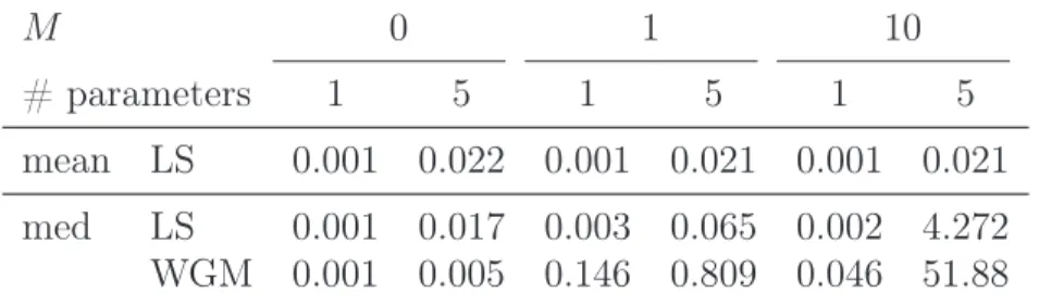
Table 1: The mean squared errors of the within-group LS and WGM estimates based on the mean and median transformations.
M 0 1 10
# parameters 1 5 1 5 1 5
mean LS 0.001 0.022 0.001 0.021 0.001 0.021 med LS 0.001 0.017 0.003 0.065 0.002 4.272 WGM 0.001 0.005 0.146 0.809 0.046 51.88
and c = 4.685. A further protection against observations with a high leverage is
provided by the location weights indirectly proportional to the values of covariates:
ˆ
wx
it = min{1,
q
χ2
p,0.975/RDit}, where χ2p,0.975 is the 97.5% quantile of the chi-square distribution withp degrees of freedom, RDit = [( ˜xit−µ)ˆ >Vˆ−1( ˜xit−µ)]ˆ 1/2 is a robust
version of the Mahalanobis distance (Rousseeuw and Zomeren, 1990), andµˆ andVˆ are
robust estimates of the location and variance matrix of x˜it. The WGM estimator is
then defined as the weighted LS (WLS) estimator for the median-transformed data
ˆ
βnT(WGM,med) = arg min β∈Rp n X i=1 T X t=1 ˆ wr itwˆxitr 2,(med) it (β). (6)
The complete WGM procedure can asymptotically achieve the breakdown point
1/4. On the other hand, WGM is neither regression nor affine equivariant and its
asymptotic distribution (even for T → ∞) has not been derived yet. The lack of
equivariance properties comes from the nonlinearity of the median transformation and
complicates the use of WGM in applications as we now demonstrate, at least if T is
small. Consider the following linear panel-data model (i= 1, . . . ,100;t = 1,2,3)
yit =x>itβ+αi+εit, (7)
(−M,0, M,0,−M)> ∈ R5. Simulating the data 1000 times and estimating the model
for M = 0,1, and 10 by LS and WGM results in the mean squared errors in Table 1.
Obviously, various levels of the multiplier M do not have any impact on the precision
of the within-group LS estimator. Using LS and WGM after removing the individ-ual effects by the median centering however leads to completely different results: the mean squared errors are substantially increasing with the magnitude of the regression coefficients, especially for the model with 5 variables.
3
New robust estimators for panel data
Because using the within-group transformation with LS is non-robust and using the
(robust) median in place of the mean (Bramati and Croux, 2007) introduces
incon-sistency when the time dimension T is small and fixed, we now propose alternative
robust estimators of β in (1) that do not rely on estimating the central tendency of
fixed effects. This will be done in two steps. First, the elimination of unobserved in-dividual effects will be addressed by considering other data transformations than the mean or median centering (Section 3.1). Second, in the light of recent contributions in robust statistical theory, LTS (Section 3.2) will be followed by new robust and efficient estimators adapted to the panel data setting (Section 3.3).
3.1
Data transformations
Since applying a robust estimate of location to centered data does not lead to a us-able estimator (see Section 2.2), we focus on the first-difference and pairwise-difference transformations instead. The first-difference transformation is already well known in
model (1) can be transformed to
∆yit=yit−yit−1 =x>itβ+εit−x>it−1β−εit−1 = ∆x>itβ+ ∆εit, (8)
where i = 1, . . . , n and t = 2, . . . , T and where no fixed effects αi appear. Under the
strict-exogeneity assumption, β is consistently estimated by LS applied to (8). This
alternative to the within-group estimator, which is the best linear unbiased
estima-tor when error terms εit are uncorrelated, is preferable if error terms εit are serially
correlated (see Wooldridge, 2002, for details).
Alternatively, one could try to obtain more accurate estimates than from (8) by eliminating individual effects by taking all pairwise differences within each individual. Inspired by Stromberg et al. (2000) and Honoré and Powell (2005), let us define the
pairwise-difference transformation as ∆sz
it = zit −zit−s, where s = 1, . . . , t−1, for
any t ∈ {2, . . . , T} and i ∈ {1, . . . , n}. Applied to model (1), the pairwise-difference transformation yields
∆sy
it=yit−yit−s = (xit−xit−s)>β+εit−εit−s = ∆sx>itβ+ ∆sεit, (9)
which removes the individual-specific variableαi similarly to (8), but generates a larger
sample sizenT(T−1)/2instead ofn(T−1)in (8) since differences for alls= 1, . . . , t−1
are considered.
To handle all transformations in a unified way, let us now introduce a more general notation. Given the original data set{xit, yit}n, Ti=1,t=1, let{x˜it,y˜it}n, T
(T)
i=1,t=1 be the data set
created by one of the considered data transformations T, T ∈ {med,1∆, P∆}, where
med,1∆, and P∆are shorthand symbols for the median-centering, first-difference, and
3.2
Initial robust estimator
Once the individual effects have been eliminated, it is of interest to find a proper robust
estimator forβin (1). Similarly to Bramati and Croux (2007), we use initially the LTS
estimator, which may be generally defined for the T-transformed data as
ˆ β(LTS,T,hnT) nT = arg min β∈Rp hnT X j=1 r(2j,()T)(β), (10)
where r(2j,()T)(β) is the jth smallest order statistics of squared residuals, the (i, t)th residual equals r(itT)(β) = ˜yit −x˜it>β, and hnT is the trimming constant, nT(T)/2 <
hnT ≤ nT(T). We assume that the trimming constant is defined so that hnT/nT(T) →
λ ∈ h1/2,1i, and thus asymptotically, the 1−λ fraction of observations is eliminated
from the objective function (10). To study the breakdown properties of the proposed LTS estimation under different transformations, let us make the following assumptions.
Assumption D
D1 Let {xit, yit}n, Ti=1,t=1 be a random sample generated according to model (1).
D2 The transformed data {x˜it,y˜it}n, T
(T)
i=1,t=1 are almost surely in a general position for
nT(T)>3(p+ 1), that is, anyp+ 1data points do not lie on the same hyperplane
almost surely.
Contrary to the median centering, both the first-difference and pairwise-difference
transformations are linear transformations of the data. Therefore, the LTS estimator
applied to such transformed data does not lose its equivariance properties contrary to LTS applied to the median-transformed data in Bramati and Croux (2007).
Lemma 1 Suppose that Assumption D1 holds. If T ∈ {1∆, P∆}, then the LTS
esti-mator βˆ(LTS,T,hnT)
Further, let now look at the breakdown properties of the LTSestimator.
Theorem 1 Suppose that Assumption D hold. Let βˆ(LTS,T,hnT)
nT be the LTS estimator defined in (10) forhnT/(nT(T))→λ as nT(T) → ∞. IfhnT ≥hT
(T)
nT = [nT(T)/2] + [(p+
1)/2] + 1, then it holds that
ε∗nT ³ ˆ β(LTS,T,hnT) nT ;{xit, yit}n, Ti=1,t=1 ´ ≥ nT (T)−h nT 2nT(T) ·κ (T)(T), (11)
where κ(1∆)= [2(T −1)]/[min{2, T −1}T]and κ(P∆)= 1. The breakdown point of LTS
tends asymptotically toκ(T)(T)(1−λ)/2, and in particular, toκ(T)(T)/4forh
nT =hT
(T)
nT .
From the breakdown point of view, both proposed data transformations are
asymp-totically equivalent for T = 2 and for T → ∞ as they yield the same maximum
breakdown point 1/4 analogously to Bramati and Croux (2007). Whereas the pairwise
differencing reaches this breakdown point for any number of time periods T, the first
differencing has a smaller breakdown point equal to (T −1)/(4T) for T ≥ 3. Let us
note that this disadvantage of the first differencing could be eliminated by considering
only differences at even time periods (e.g., ∆y2,∆y4, . . .): the breakdown point would
asymptotically equal1/4irrespective ofT, but the precision of estimation would suffer.
3.3
Robust and efficient estimation
Since theLTSestimator with the maximum breakdown point achieves only 8% relative
efficiency for normally distributed data, one-step estimators are often employed to im-prove the precision of estimation without substantially affecting the robust properties of estimation (see also Section 2.2).
To introduce the efficient one-step methods, suppose we have the transformed data
estimators of the regression parameters βˆ0
nT and residual scale σˆnT0 (e.g., the median
absolute deviation). A classical example of a one-step augmentation procedure is the
iteratively reweightedLS (IRLS) estimator proposed by Rousseeuw and Leroy (1987),
which removes the observations having large absolute residuals according to some initial robust fit and then applies LS. Denoting the initial residualsrit(T)( ˆβ0
nT) = ˜yit−x˜>itβˆnT0 ,
one can thus define weights
ˆ wit ³ ˆ β0 nT,σˆ0nT;v ´ =I ³ |rit(T)( ˆβ0 nT)/σˆnT0 |< v ´ (12)
for a constant v > 0 (e.g., Gervini and Yohai (2002) suggest v = 2.5). The IRLS
estimator then reads as follows:
ˆ
β(IRLSnT ,T)= arg min β∈Rp n X i=1 T(T) X t=1 ˆ wit ³ ˆ β0 nT,σˆnT0 ;v ´ rit2,(T)(β). (13)
A data-adaptive version of (13) designed to achieve efficiency for normally
dis-tributed data, the robust and efficient weighted least squares (REWLS) estimator, has
been proposed by Gervini and Yohai (2002). A data-dependent cut-off point vˆnT to
define weights (12) is now determined by comparing two distribution functions,F+and
F0+, where the former relates to the standardized absolute residuals|r(itT)( ˆβ0
nT)/σˆnT0 |and
the latter is the distribution function assumed for these standardized absolute residuals
in the model (1). SinceF+ is usually unknown, it is estimated by the empirical
distri-bution function F+
nT of |r
(T)
it ( ˆβnT0 )/σˆnT0 |. The maximum discrepancy dˆnT between FnT+
and F+
0 in the tail of the distributions can be then measured by
ˆ
dnT = sup v≥η
©£
F0+(v)−FnT+(v)¤·I¡F0+(v)−FnT+(v)≥0¢ª, (14)
where η is a large quantile of F+
F0 ≡N(0,1)(see Gervini and Yohai, 2002). The cutoff pointvˆnT is then defined as the
(1−dˆnT)th quantile of the distribution FnT+: vˆnT = min
©
v |F+
nT(v)≥1−d0
ª
.Finally, the REWLSestimator is obtained from (13) for v = ˆvnT ≥η:
ˆ
β(REWLSnT ,T)= arg min β∈Rp n X i=1 T(T) X t=1 ˆ wit ³ ˆ βnT0 ,σˆnT0 ; ˆvnT ´ rit2,(T)(β). (15)
This method is proved to preserve the breakdown-point properties of the initial robust estimator and achieve the asymptotic efficiency for Gaussian errors.
An alternative to the traditional one-step estimators is the reweighted least trimmed
squares (RLTS) estimator (Čížek, 2010). Similarly to Gervini and Yohai (2002), weights
(12) are constructed using the data-dependent cutoff point vˆnT. The resulting weights
are however used within theLTSestimator rather than LS. SinceLTSrequires only the
total numberhnT of observations to be included in the objective function, the number
of observations with non-zeros weightswˆit(·,·; ˆvnT) has to be counted:
ˆ hnT = n X i=1 T(T) X t=1 I ³¯¯ ¯r(itT) ³ ˆ β0 nT ´ /σˆ0 nT ¯ ¯ ¯<vˆnT ´ = n X i=1 T(T) X t=1 ˆ wit ³ ˆ β0 nT,σˆ0nT; ˆvnT ´ (16)
The RLTS estimator is then simply defined as LTS using the data-dependent amount
of trimming ˆhnT applied to the T-transformed panel data:
ˆ βnT(RLTS,T)= arg min β∈Rp ˆ hnT X j=1 r2(j,()T)(β). (17)
Similarly to REWLS, RLTS preserves the breakdown-point properties of the initial
robust estimator. Additionally, RLTSis asymptotically independent of the initial
esti-mator and achieves asymptotic efficiency when errors are normally distributed. Let us now formally state the breakdown properties of these one-step estimators.
Theorem 2 Assume that Assumption D holds and that the data have been transformed according to one of theT-transformations,T∈ {1∆, P∆}. Further, letε0∗
nT be the finite-sample breakdown point of the initial estimator βˆ0
nT of the regression parameters with limit ε0∗ = lim
n→∞ε0nT∗. Additionally, suppose σˆ0nT = MADi,trit( ˆβnT0 )/Φ−1(3/4) is the standardized median absolute deviation estimator and F0 has a finite variance. Then it
holds that ε∗ nT( ˆβ (IRLS,T) nT )≥ε0nT∗, ε∗nT( ˆβ (REWLS,T) nT )≥ε0nT∗, and ε∗nT( ˆβ (RLTS,T) nT )≥ε0nT∗.
Thus, we see that all one-step methods –WGM,REWLSandRLTS– have the same
breakdown properties. Note that this holds even though IRLS does not use weightswˆx
it
in constrast to WGM. The different methods could differ though by the bias caused by outliers and in their finite-sample and asymptotical variances.
3.4
Asymptotic properties
The estimators introduced in the previous sections are applied to model (1) after the first-difference or pairwise-difference transformations, which lead to the serial correla-tion of the errors in (8) or (9), respectively. Almost all robust regression estimators are however asymptotically studied under the assumption of independent (and often iden-tically distributed) errors, be it in the context of cross-sectional (Gervini and Yohai, 2002) or panel data (Lucas et al., 2007), or there are no asymptotic results available (Bramati and Croux, 2007; Dhaene and Zhu, 2009). This limits also the extent to which we can characterize the asymptotic distribution of the proposed estimators. In particular, the asymptotic distribution under the first- and pairwise-differences can be easily derived only for the initial LTS estimator and its reweighted form RLTS (with the notable exception of the estimation based only on the first differences taken at even time periods as mentioned in Section 3.2, which produces independent errors).
Now, the assumptions necessary to derive the asymptotic distribution of LTS and RLTS are presented. To this end, let Xi = (xi1, . . . ,xiT)>, yi = (yi1, . . . , yiT)>, X˜i =
( ˜xi1, . . . ,x˜iT(T))>, y˜i = (˜yi1, . . . ,y˜iT(T))>, and ε˜it = ˜yit −x˜itβ0 for all i ∈ N and t = 1, . . . , T(T), whereβ0is the true parameter value in model (1). Further, let us recall that, in this context,λ∈ h1/2,1irefers to the limitslimn→∞hnT/nT(T)orlimn→∞ˆhnT/nT(T),
see (16), and that T ≥ 2 is a fixed integer. The assumptions and the asymptotic
distribution will be stated for symmetrically distributed errors for the sake of simplicity. A more general result can be found in Čížek (2010), where a detailed discussion of these assumptions can be found.
Assumption A
A1 Random vectors yi and matrices Xi are independent and identically distributed
for all i∈Nand have finite second moments.
A2 Let {εit}i∈N be a sequence of random variables with finite second moments and
E(εit|Xi) = 0 for all i ∈ N and t = 1, . . . , T. Further, the unconditional
dis-tribution function F of εit is assumed to be unimodal, absolutely continuous,
and symmetrically distributed condionally on Xi. Its density function has to be
bounded and continuously differentiable.
A3 LetQ(λ) = E[ ˜X>
i diag({I[|F(˜εit)−F(−ε˜it−2C)| ≤ λ]}T
(T)
t=1 ) ˜Xi] be a nonsingular
matrix for any fixed C ∈R.
A4 Denoting Gβ and gβ the unconditional cumulative distribution and density
func-tions of (˜yit−x˜>itβ)2, let supβ∈Rpsupz>αgβ(z) <∞ for any α > 0, and if λ <1,
that infβ∈Rpinfz∈(−δ,δ)gβ
¡
G−1
β (λ) +z
¢
>0for some δ >0.
Assumption A1 formulates standard conditions of the (uniform) central limit the-orem: observed variables are independent across cross-sectional units and have finite
second moments. Assumption A2 presents the assumptions on the error termεit, which
the most general case, only the second moments of the trimmed errors ei(qλ) defined
below have to be finite (see Čížek, 2011). Next, Assumption A3 formulates an analog of the standard full-rank condition, and is actually equivalent to E( ˜XiX˜i>) > 0 if ε˜it
is independent ofXi. Finally, Assumption A4 formalizes the fact that the distribution
of squared residuals should be absolutely continuous: its density should not approach
∞at any point, which would correspond to the distribution becoming discontinuous at
some point. If ε˜it is independent of x˜it, Assumption A4 is usually implied by F being
absolutely continuous with a density function f positive, bounded and differentiable
(Čížek, 2006).
Under Assumption A, Čížek (2010) derived the below stated result regarding the
asymptotic distribution of LTS and RLTS. To formulate this result, the notation qλ =
p
G−1(λ) is used, where G ≡ G0
β and G−1 represents the unconditional quantile
function of ε˜2
it. Additionally, one diagonal matrix and two vectors depending on qλ
are needed: Ii(qλ) = diag[{I(˜εit ≤ qλ)}T
(T)
t=1 ], ei(qλ) = Ii(qλ)(˜εi1, . . . ,ε˜iT(T))>, and fi(qλ) = (fi1(qλ), . . . , fiT(T)(qλ))>, where fit is the conditional distribution of ε˜it|X˜i.
Theorem 3 Let Assumption A hold. Next, let Σ(λ) = E[ ˜X>
i {ei(qλ)ei(qλ)>}X˜i],
Q(λ) = E[ ˜X>
i Ii(qλ) ˜Xi], J(λ) =−E[qλX˜i>diag{fi(−qλ) +fi(qλ)}X˜i], andQ(λ) +J(λ) be a non-singular matrix. Then the (reweighted) LTS estimator βˆnT(RLTS,T) defined by trimming ˆhnT such that limn→∞ˆhnT/nT →λ for some λ ∈ h1/2,1i is a
√
n-consistent and asymptotically normal, √n( ˆβnT(RLTS,T)−β0) →L N(0, V(λ)) as n → ∞, where the
asymptotic covariance matrix equals V(λ) = {Q(λ) +J(λ)}−1Σ(λ){Q(λ) +J(λ)}−1.
The theorem covers not only the reweighted, but also the initial LTS estimator
for hˆnT = hnT = const. Consequently, the initial and reweighted LTS estimators are
asymptotically normal. The estimation of their covariance matrix V(λ) is discussed in
4
Simulation study
This section contains a simulation study of the finite-sample properties of some pro-posed and existing panel-data estimators. The following simulations are meant to in-vestigate the behavior of estimators when the sample dimensions vary (Section 4.1), when errors come from various error distributions (Section 4.2), and when different kinds of outlying observations are present (Section 4.3). The reference estimator is the
within-group estimator βˆ(LSnT,mean). Other estimators under consideration are the LS,
LTS with the maximum amount of trimming (see Theorem 1), WGM of Bramati and
Croux (2007), IRLS, REWLS, and RLTSestimators subject to three data
transforma-tions T ∈ {med,1∆, P∆}. Let us recall that WGM and IRLS are both based on the
same reweighted LS method, but differ by employed weights: WGM uses a continous weighting function and downweights observations with large covariates, whereas IRLS uses 0–1 weights determined only by absolute residuals similarly to REWLS and RLTS.
The data generating process is given by a static fixed-effect panel-data model
yit =x>itβ+αi+εit, αi = T X t=1 x> itγ/ √ T +ηi, i= 1,· · · , n, t = 1,· · · , T, (18)
where the εit’s are independent and identically distributed according to some
distri-bution H. The parameters of interest are chosen β = (1,0,−1)>. The
unobserv-able individual effects αi depend on ηi ∼ U(0,12) and on the covariates xit through
γ= (2,2,2)>. Observable covariates x
it’s are generated according to
xitk ∼ χ2 2−2 if k= 1, N(0,1) if k≥2, (19)
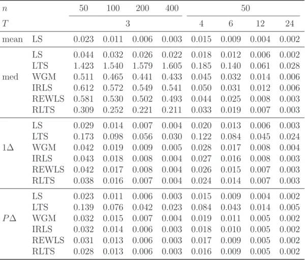
Table 2: The mean squared errors of all estimators for normally distributed errors and various sample sizes.
n 50 100 200 400 50 T 3 4 6 12 24 mean LS 0.023 0.011 0.006 0.003 0.015 0.009 0.004 0.002 LS 0.044 0.032 0.026 0.022 0.018 0.012 0.006 0.002 LTS 1.423 1.540 1.579 1.605 0.185 0.140 0.061 0.028 med WGM 0.511 0.465 0.441 0.433 0.045 0.032 0.014 0.006 IRLS 0.612 0.572 0.549 0.541 0.050 0.031 0.012 0.006 REWLS 0.581 0.530 0.502 0.493 0.044 0.025 0.008 0.003 RLTS 0.309 0.252 0.221 0.211 0.033 0.019 0.007 0.003 LS 0.029 0.014 0.007 0.004 0.020 0.013 0.006 0.003 LTS 0.173 0.098 0.056 0.030 0.122 0.084 0.045 0.024 1∆ WGM 0.042 0.019 0.009 0.005 0.028 0.017 0.008 0.004 IRLS 0.043 0.018 0.008 0.004 0.027 0.016 0.008 0.003 REWLS 0.042 0.017 0.008 0.004 0.026 0.015 0.007 0.003 RLTS 0.038 0.016 0.007 0.004 0.024 0.014 0.007 0.003 LS 0.023 0.011 0.006 0.003 0.015 0.009 0.004 0.002 LTS 0.139 0.076 0.042 0.023 0.084 0.043 0.014 0.005 P∆ WGM 0.032 0.015 0.007 0.004 0.019 0.011 0.005 0.002 IRLS 0.032 0.014 0.006 0.003 0.018 0.010 0.005 0.002 REWLS 0.031 0.013 0.006 0.003 0.017 0.009 0.005 0.002 RLTS 0.028 0.013 0.006 0.003 0.016 0.009 0.005 0.002
where xitk denotes the kth component of xit, k = 1,2,3, χ22 denotes the chi-squared
distribution with 2 degrees of freedom, and N(0,1) represents the standard normal
distribution.
Simulation experiments are conducted across different sample sizes nT, aiming at
both short micro-panels and long macro-panels, with n and T ranging from (n, T) =
(100,3) to (n, T) = (50,24). The performance of each estimator is evaluated using
S= 1000simulated samples and is measured by the mean squared error (MSE):MSE = 1/SPSs=1kβˆs
nT − βk2, where βˆnTs , s = 1, . . . , S, are the estimates for S simulated
4.1
Sample sizes
The performance of the estimators is first evaluated for normal errors, H ≡ N(0,1),
at different sample sizes: for T fixed and n increasing and for T increasing while n is
fixed. The simulation results are summarized in Table 2. The results for the median transformation confirm that the robust estimators based on this transformation are not
consistent for a fixed number of time periods T, but are consistent if T → ∞. Next,
LTS performs much worse than LS for all transformations, while all one-step estimators (WGM, IRLS, REWLS, and RLTS) exhibit much smaller MSEs and can match the performance of LS if the sample size is sufficiently large. Finally, it is interesting to note that – while the within-group LS estimator outperforms the LS applied to first-differenced data (errors are iid) – the LS and one-step robust estimators applied to pairwise-differenced data can actually match the performance of the within-group LS estimator.
4.2
Different error distributions
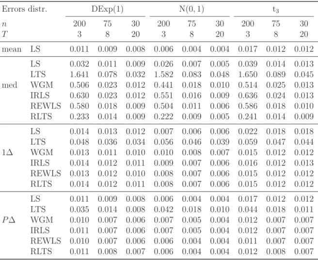
In this subsection, three different distributions H of the error term εit in (18) are
considered: the standard normalN(0,1), the double exponential distributionDExp(1)
with rate 1, and the Student distribution t3 with 3 degrees of freedom, see Table 3.
The LS estimator is no longer optimal and is slightly outperformed by one-step robust estimators in the case of the double-exponential errors and more substantially in the case of the Student errors (the differences among WGM, IRLS, REWLS, and RLTS are practically negligible). Regarding the data transformations, the pairwise-differencing leads uniformly to the best results, and in combination with REWLS, is preferable to the within-group LS estimator.
Table 3: The mean squared errors of all estimators for errors from the standard normal, double exponential, and Student distributions.
Errors distr. DExp(1) N(0,1) t3
n 200 75 30 200 75 30 200 75 30 T 3 8 20 3 8 20 3 8 20 mean LS 0.011 0.009 0.008 0.006 0.004 0.004 0.017 0.012 0.012 LS 0.032 0.011 0.009 0.026 0.007 0.005 0.039 0.014 0.013 LTS 1.641 0.078 0.032 1.582 0.083 0.048 1.650 0.089 0.045 med WGM 0.506 0.023 0.012 0.441 0.018 0.010 0.514 0.025 0.013 IRLS 0.630 0.023 0.012 0.551 0.016 0.009 0.636 0.024 0.013 REWLS 0.580 0.018 0.009 0.504 0.011 0.006 0.586 0.018 0.010 RLTS 0.233 0.014 0.009 0.222 0.009 0.005 0.241 0.014 0.009 LS 0.014 0.013 0.012 0.007 0.006 0.006 0.022 0.018 0.018 LTS 0.048 0.036 0.034 0.056 0.046 0.039 0.059 0.047 0.044 1∆ WGM 0.013 0.011 0.010 0.010 0.008 0.007 0.015 0.012 0.012 IRLS 0.014 0.012 0.011 0.009 0.007 0.006 0.016 0.012 0.013 REWLS 0.013 0.012 0.010 0.008 0.007 0.006 0.015 0.012 0.012 RLTS 0.014 0.012 0.011 0.008 0.007 0.006 0.015 0.012 0.012 LS 0.011 0.009 0.008 0.006 0.004 0.004 0.017 0.012 0.012 LTS 0.035 0.014 0.008 0.042 0.018 0.010 0.044 0.018 0.011 P∆ WGM 0.010 0.007 0.006 0.007 0.005 0.004 0.012 0.007 0.007 IRLS 0.011 0.007 0.006 0.007 0.005 0.004 0.012 0.007 0.007 REWLS 0.010 0.007 0.006 0.006 0.004 0.004 0.011 0.007 0.007 RLTS 0.011 0.008 0.007 0.006 0.004 0.004 0.012 0.008 0.007
4.3
Outliers
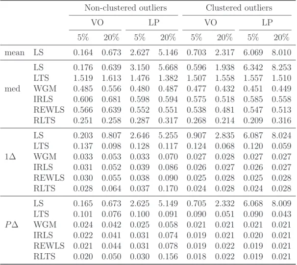
The robust properties are now evaluated by including outliers in the data. Let m
be the number of outliers and let Im be the index set of contaminated observations.
Contaminated values of the dependent variableyˇr
it ∼U(−10,30)oryˇitc ∼U(29,30)and
independent variables xˇitk ∼ N(6,2), (i, t) ∈ Im, k = 1,2,3, result in the following
contamination schemes defined by the actual values of (xit, yit) for (i, t) ∈ Im. If
yit = ˇyitr or yit = x>itβ+αi + ˇyitc for (i, t) ∈ Im, we talk about the non-clustered and
clustered outliers, respectively. On the other hand, ifxitis left unmodified orxit= ˇxit,
the contamination schemes is said to contain vertical outliers (VO) or leverage points
(LP), respectively. All non-contaminated data (i, t)6∈ Im follow model (18)–(19) with
H ≡ N(0,1). The sample size is fixed to n = 70 and T = 3 now and the number of
outliers is set to m= 10 (5% contamination) and m= 42 (20% contamination).
The results summarized in Table 4 document that, even if only 5% observations are contaminated, LS can get extremely biased (actually more that the inconsistent estimators based on the median transformation). On the contrary, the proposed robust estimators are not substantially affected by any type of contamination. Similarly to experiments discussed in previous sections, there are no substantial differences among the one-step robust estimators, while the data transformation matters: the pairwise-differencing again outperforms the first-pairwise-differencing.
5
Concluding remarks
The present study examines the parameter estimation in fixed-effects panel data mod-els with a fixed number of time periods from the point of view of robust statistical procedures. To achieve consistent estimators, we privilege first-difference and propose pairwise-difference data transformations and then apply robust estimators: LTS
fol-Table 4: The mean squared errors of all estimators in the presence of 5% or 20% scattered and clustered outliers.
Non-clustered outliers Clustered outliers
VO LP VO LP 5% 20% 5% 20% 5% 20% 5% 20% mean LS 0.164 0.673 2.627 5.146 0.703 2.317 6.069 8.010 LS 0.176 0.639 3.150 5.668 0.596 1.938 6.342 8.253 LTS 1.519 1.613 1.476 1.382 1.507 1.558 1.557 1.510 med WGM 0.485 0.556 0.480 0.487 0.477 0.432 0.451 0.449 IRLS 0.606 0.681 0.598 0.594 0.575 0.518 0.585 0.558 REWLS 0.566 0.639 0.552 0.551 0.538 0.481 0.547 0.513 RLTS 0.251 0.258 0.287 0.317 0.268 0.214 0.209 0.316 LS 0.203 0.807 2.646 5.255 0.907 2.835 6.087 8.024 LTS 0.137 0.098 0.128 0.117 0.124 0.068 0.120 0.059 1∆ WGM 0.033 0.053 0.033 0.070 0.027 0.028 0.027 0.027 IRLS 0.031 0.052 0.039 0.086 0.026 0.027 0.026 0.027 REWLS 0.030 0.055 0.038 0.090 0.025 0.028 0.025 0.028 RLTS 0.028 0.064 0.037 0.170 0.024 0.028 0.024 0.028 LS 0.165 0.673 2.625 5.149 0.705 2.332 6.068 8.009 LTS 0.101 0.076 0.100 0.091 0.090 0.051 0.090 0.043 P∆ WGM 0.024 0.042 0.025 0.058 0.021 0.021 0.021 0.021 IRLS 0.022 0.041 0.031 0.074 0.019 0.021 0.020 0.021 REWLS 0.021 0.044 0.031 0.078 0.019 0.022 0.019 0.021 RLTS 0.020 0.050 0.030 0.156 0.018 0.022 0.019 0.021
lowed by various reweighted LS and LTS methods. For a given data transformation, all methods achieve the same breakdown point and have similar finite-sample perfor-mance; the asymptotic distribution could be however provided only in the case of LTS and RLTS. Comparing the two data transformations, the best robust properties (i.e.,
the breakdown point 1/4 irrespective of the number of time periods T) and the best
estimation results have been obtained for the new pairwise-difference transformation, which could motivate its further study in the context of panel data models.
APPENDIX: PROOFS
Proof of Lemma 1: Since the LTS estimator is regression, affine, and scale equiv-ariant (Rousseeuw and Leroy, 1987, Lemma 3 in Chapter 3), we only have to verify that the data-transformations – the first- and pairwise-differencing – do not affect the
regression, affine, and scale transformations. For any s∈ N, this directly follows from
∆s(cy
it) = c∆syit, ∆s(yit+x>itv) = ∆syit+ (∆sxit)>v, and ∆s(x>itA) = (∆sxit)>A. ¤
Proof of Theorem 1: Before applying the LTSestimator, data are subject to the
differencing transformations (8) or (9), which generateT(T) =n(T−1)orT(T) =nT(T−
1)/2 transformed observations, respectively. With these transformations, the worst
case scenario occurs when aberrant observations are located so that each single outlier
contaminates always min{2, T −1} (first-differencing) orT −1 (pairwise-differencing)
differentiated observations. Hence givenm outliers in the original sample, the number
of outliers after the first- and pairwise-differencing will be at mostmin{2, T −1}m and
(T −1)m, respectively.
At the same time, the breakdown point of LTS with the trimming constant hnT
equals (nT(T)−h
nT)/[nT(T)] if hnT ≥ (nT(T)+p+ 1)/2 (Vandev and Neykov, 1998).
LTS thus breaks down only if the number of outliers exceedsnT(T)−h
nT. In the case of
the first differences, this means that LTS breaks down ifmin{2, T−1}m > nT(T)−h
nT,
implying that the breakdown point of the proposed panel-data LTS estimator equals
(nT(T)−h
nT)/[min{2, T−1}nT] ={(nT(T)−hnT)/[2nT(T)]} · {(2(T −1))/(min{2, T−
1}T)}. In the case of the pairwise differences, LTS breaks down if (T − 1)m >
nT(T) −h
nT, implying that the breakdown point equals (T(T) − hTn)/[nT(T − 1)] =
(nT(T)−h
nT)/(2nT(T)). The last claim of the theorem follows from limn→∞(nT(T)−
hnT)/(2nT(T)) = (1−λ)/2. ¤
Proof of Theorem 2: The claim of the theorem is proved for REWLS by Gervini and Yohai (2002, Theorem 3.3) and for RLTS by Čížek (2010, Theorem 2). The result
for the IRLS estimator also directly follows from Gervini and Yohai (2002, Theorem
3.3), sincevnT determined by REWLS is by definition always greater or equal tov =η
used in (12), see equation (14). ¤
References
Bramati, M. C. and C. Croux (2007). Robust estimators for the fixed effects panel data
model. Econometrics Journal 10(3), 521–540.
Čížek, P. (2006). Least trimmed squares in nonlinear regression under dependence.
Journal of Statistical Planning and Inference 136(11), 3967–3988.
Čížek, P. (2008). Robust and efficient adaptive estimation of binary-choice regression
models. Journal of the American Statistical Association 103, 687–696.
Čížek, P. (2010). Reweighted least trimmed squares: an alternative to one-step estima-tors. Discussion Paper 91/2010, CentER, Tilburg University.
Čížek, P. (2011). Semiparametrically weighted robust estimation of regression models.
Computational Statistics and Data Analysis 55, 774–788.
Davies, P. L. and U. Gather (2005). Breakdown and groups. The Annals of
Statis-tics 33(3), 977–1035.
Dhaene, G. and Y. Zhu (2009). Median-based estimation of dynamic panel models with fixed effects. Working paper, Faculty of Business and Economics, Katholieke Universiteit Leuven.
Genton, M. G. and A. Lucas (2003). Comprehensive definitions of breakdown points for
independent and dependent observations. Journal Of The Royal Statistical Society
Gervini, D. and V. J. Yohai (2002). A class of robust and fully efficient regression
estimators. The Annals of Statistics 30(2), 583–616.
Hampel, F. R., E. M. Ronchetti, P. J. Rousseeuw, and W. A. Stahel (1986). Robust
statistics : the approach based on influence functions. John Wiley & Sons.
Honoré, B. E. and J. L. Powell (2005). Pairwise difference estimation of nonlinear
models. In D. W. K. Andrews and J. H. Stock (Eds.), Identification and Inference
for Econometric Models. Essays in Honor of Thomas Rothenberg., Chapter 22, pp. 520–553. Cambridge University Press.
Koenker, R. (2004). Quantile regression for longitudinal data. Journal of Multivariate
Analysis 91(1), 74–89.
Lucas, A., R. van Dijk, and T. Kloek (2007). Outlier robust gmm estimation of leverage determinants in linear dynamic panel data models. Unpublished manuscript.
Maronna, R. A., R. D. Martin, and V. J. Yohai (2006). Robust Statistics. John Wiley
& Sons.
Maronna, R. A. and V. J. Yohai (2000). Robust regression with both continuous and
categorical predictors. Journal of Statistical Planning and Inference 89(1-2), 197–
214.
Ronchetti, E. and F. Trojani (2001). Robust inference with gmm estimators. Journal
of Econometrics 101(1), 37–69.
Rousseeuw, P. J. (1984). Least median of squares regression. Journal of the American
Statistical Association 79(388), 871–880.
Rousseeuw, P. J. and A. M. Leroy (1987). Robust regression and outlier detection.
Rousseeuw, P. J. and B. C. v. Zomeren (1990). Unmasking multivariate outliers and
leverage points. Journal of the American Statistical Association 85(411), 633–639.
Simpson, D. G., D. Ruppert, and R. J. Carroll (1992). On one-step gm estimates
and stability of inferences in linear regression. Journal of the American Statistical
Association 87(418), 439–450.
Stromberg, A. J., O. Hossjer, and D. M. Hawkins (2000). The least trimmed differences
regression estimator and alternatives. Journal of the American Statistical
Associa-tion 95(451), 853–864.
Vandev, D. L. and N. M. Neykov (1998). About regression estimators with high
break-down point. Statistics 32, 111–129.
Wagenvoort, R. and R. Waldmann (2002). On b-robust instrumental variable estimation
of the linear model with panel data. Journal of Econometrics 106(2), 297–324.
Wooldridge, J. M. (2002). Econometric Analysis of Cross Section and Panel Data,