Machine learning for crystal identification and discovery

Author Manuscript

Machine learning for crystal identification and discovery

Matthew Spellings

and Sharon C. Glotzer

1

Department of Chemical Engineering, University of Michigan, Ann Arbor, MI 48109

Biointerfaces Institute, University of Michigan, Ann Arbor, MI 48109

March 12, 2018

Abstract

As computers get faster, researchers — not hardware or algorithms — become the bottleneck in scientific discovery. Computational study of colloidal self-assembly is one area that is keenly affected: even after computers generate massive amounts of raw data, performing an exhaustive search to determine what (if any) ordered structures occur in a large parameter space of many

simulations can be excruciating. We demonstrate how machine learning can be applied to

discover interesting areas of parameter space in colloidal self-assembly. We create numerical fingerprints — inspired by bond orientational order diagrams — of structures found in self-assembly studies and use these descriptors to both find interesting regions in a phase diagram and identify characteristic local environments in simulations in an automated manner for simple and complex crystal structures. Utilizing these methods allows analysis to keep up with the data generation ability of modern high-throughput computing environments.

Keywords: machine learning, data science, computational, self-assembly, crystal

∗_{[email protected]}

This contribution was identified by Andrew Ferguson (University of Illinois at Urbana-Champaign) as the Best Presentation in the session “Data Mining and Machine Learning in Molecular Sciences I” of the 2016 AIChE Annual Meeting in San Francisco.

Author Manuscript

Introduction

In the process of engineering the self-assembly behavior of colloidal- and nanoscale particles, scientists leave enormous amounts of configurational data in their wake. Experimentally, crystal

structures with tunable properties can be created through anisotropic colloidal building blocks1_,

DNA-coated nanoparticles2,3,4, or a host of other interactions5. In computational studies of

colloidal matter, various simple, as well as complex, phases can be formed through systematic

modification of entropic or enthalpic interparticle interactions6,7,8,9,10,11_{. For exploratory studies}

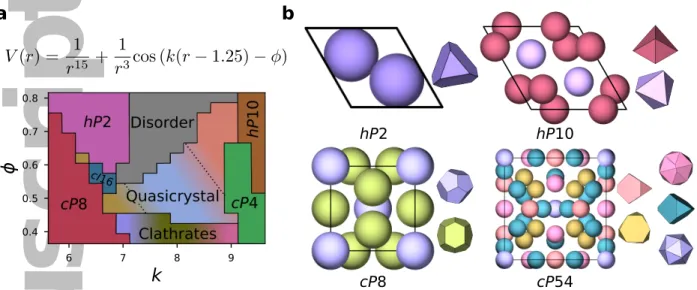
of these parameter spaces, the design process is difficult: after the computationally expensive undertaking of performing simulations, each dataset must also be analyzed — a procedure that is often manual, repetitive, and labor-intensive in the case of crystal structure identification. This analysis difficulty is partly due to the wide variety of crystal structures that can be found in self-assembling systems, as shown in Figure 1. As advances in hardware and software conspire to decrease the cost of parallel computation, it will only become more imperative that researchers utilize automated, high-performance analysis methods to investigate the data generated from their high-throughput simulation codes.

Automated analysis of data from two-dimensional systems has been successfully performed

using variations on then-atic order parameter(s)ψn, defined for each particle as12,13

ψn= 1 n ∑ j einθij_.

where the sum is over particle i’s neighbors and θij is the angle of the bond between particle

iand particle j. ψn can identify tetratic and hexatic behavior in hard squares14, rectangles15,

and disks12,13, as well as hexagonal order in systems of active disks16. In general, this order

parameter works well for detecting localn-fold bond orientational ordering in two-dimensional

systems, as evidenced by its wide use in these applications. In three spatial dimensions, however, structural order can be more complex, and detecting it more challenging. The Steinhardt order

parameter(s)17 _Q

n are natural three-dimensional analogues to then-atic order parameters and

they have been used to analyze many systems assembling relatively simple structures17,18,19_,

but they have some shortcomings. Even for some of the simplest, most common structures we

find in self-assembly, Steinhardt order parametersQn (and the related family of order

param-eters Wn, also derived from combinations of neighbor-bond spherical harmonics) often poorly

Author Manuscript

formed by dissimilar pairwise interactions20_{. Usually the inputs to Steinhardt order parameters}

for selection of neighbor shells, as well as threshold values for recognizing particles as being crystalline must be carefully tuned by hand to optimize the specificity for each system they will

be used to identify17,21,22_{. Ideally, the order parameters we use would be more robust and less}

biased if driven by the data we are interested in rather than arbitrary choices of symmetries to search for and hand-picked threshold values for the chosen parameters.

Another problem that hinders automatic structure analysis is that we typically do not know which structures are present in a dataset before analyzing it exhaustively. This can be problem-atic even for simple systems. For example, hard particles — which have some of the simplest interactions to define — are known to self-assemble into a great diversity of complex structures,

including quasicrystals and crystals with many-atom repeat units23,10_{. Creating and tuning}

high-specificity order parameters by hand for each of these structures would be an onerous task. Rather than designing and optimizing parameters manually, we endeavor to create generic descriptions of local symmetry and to utilize machine learning methods, in conjunction with simulation data, to automatically formulate appropriate order parameters for the structures we find. Here we will show that we can use machine learning methods to cluster data into sets of similar structures before the structures have been identified, or to identify systems quickly and efficiently given a set of known structures.

Machine learning (ML) has proven to be a powerful tool in many different fields. Typically, researchers use domain-specific knowledge to create a set of “descriptors” which place the data of interest in some high-dimensional space that the ML algorithms can work in. These descrip-tors should represent the important aspects and invariants of the systems we wish to study. In the field of soft matter, researchers have created ML models using descriptors that are sensitive

to particle coordination and local bond angles to identify crystalline phases24,25,26 _{and glassy}

solids27 respectively. One review paper28 presents an overview of families of descriptors and

order parameters with applications to condensed matter systems. For the study of colloidal self assembly, once we evaluate a set of descriptors for our data, we can apply standard ma-chine learning methods to solve the problems that interest us. In this paper, we present the use of neighborhood-local spherical harmonics, inspired by Bond Orientational Order (BOO)

analysis29,30,23,28,10_{, as descriptors of local particle environments that are sensitive to}

three-dimensional symmetries. We demonstrate the usefulness of these descriptors by analyzing data

Author Manuscript

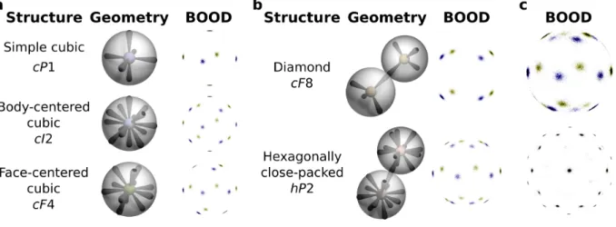
Bond Orientational Order Analysis

A common method of evaluating the structure of simulated systems is to compare Bond

Ori-entational Order Diagrams (BOODs)29,30,23,28,10 _{to those of reference structures. In a BOOD,}

the bonds — or vectors drawn between particles, typically within the first neighbor shell — of all the particles in the system are globally projected in a histogram on the surface of the unit sphere, as shown in Figure 2. Much like a diffraction pattern, the BOOD description of a system can be informative in analyzing the symmetry and quality of a crystal. However, BOOD analysis involves three caveats: first, because the BOOD is a superposition of all local crystalline environments in the global reference frame, the presence of different crystal grains — each with their own orientation — can hinder identification of structures. In the best case this is merely an annoyance, and in the worst case it can lead to the misidentification of a structure. For example, the BOOD of an ABC layered face-centered cubic (FCC) crystal with a stacking fault can appear very similar to the BOOD of an AB layered hexagonally close-packed (HCP) structure, as shown in Figure 2(c). Similarly, FCC structures can also be icosahedrally

twinned31, which causes the BOOD to exhibit icosahedral symmetry, again leading to structure

misidentification. Second, because the orientation of a BOOD is tied to the orientation of the

crystal it comes from, point-matching or symmetry detection algorithms28 _{would need to be}

employed to automatically compare a new sample to reference BOODs or find high-symmetry axes. Finally, BOODs are graphical metrics and can thus be difficult to quantitatively compare between samples and structures.

In this work we retain the idea of viewing projections of near-neighbor bonds, but rather than arranging them based on the global orientation of the crystal, we orient the bonds of each particle by a local measure: the principal axes of rotation (the eigenvectors of the inertia tensor) of its local neighborhood.

Local Neighborhood Descriptors

For structural analysis, global rotational invariance is one of the most basic properties we require of an order parameter. If the order parameters we generate are sensitive to sample orientation, they will be less helpful when identifying the same structure in two different systems, which may have crystallized with two distinct orientations. Ideally, identical bulk structures with different global orientations — or even within the same system in polycrystalline samples —

Author Manuscript

would be indistinguishable given only the values of the order parameters we create. For crystals of anisotropic particles, a good choice of local reference frame could be based on the orientation of the reference particle; however, in plastic crystals this information would be less useful due to the rotational freedom of the particles and, in general, this idea is not applicable to point particles.

To achieve global rotational invariance in our algorithm using only local information and without assuming that particles are anisotropic, we orient each particle’s local environment

based on the principal axes of rotation of its nearest neighbors1_{, represented as point masses. For}

a given number of nearest neighborsNnaround particle i, the inertia tensor of the neighborhood

is ¯ I(i, Nn) = Nn ∑ j=1 (r⃗ij·r⃗ij)¯1−r⃗ij⊗r⃗ij

wherer⃗ij is the vector from particlei’s position to the position of itsjth nearest neighbor, ¯1 is

the identity tensor, and⊗is the tensor product. We then rotate the points into the principal

reference frame for each particle, where the inertia tensor of the neighborhood is diagonal. We

accomplish this by finding the eigenvaluesλi and corresponding eigenvectors v⃗i of the inertia

tensor. We orient the structure such that the eigenvector with the largest eigenvalue (and

moment of inertia) is in thez-direction, the second-largest in they-direction, and the smallest

in thex-direction.

Using the inertia tensor to orient the local environment involves three details. First, the

result of the diagonalization procedure depends strongly on the number of particlesNn in the

local neighborhood and the symmetry of the structure being studied. For machine learning algorithms, which are often used for very high-dimensional data, we simply concatenate the de-scriptors computed for several different neighborhood sizes. Second, when the inertia tensor has repeated eigenvalues, diagonalization orients the neighborhood with one (two identical eigen-values) or two (three identical eigeneigen-values) remaining degrees of freedom randomly distributed, placing bonds randomly in rings or on the surface of the sphere, respectively. In the latter case both ordered and disordered structures exhibit no distinct intensity peaks, but we emphasize that this only occurs for particular combinations of structure and neighborhood size, so when descriptors are computed for machine learning applications — using a range of neighborhood

1_{The N nearest neighbors of particle with index iare the N distinct particles with smallest Euclidean distance}

Author Manuscript

sizes — this ambiguity is not an issue. Finally, in ordered systems with well defined shells of nearest-neighbor particles, there is often a degeneracy in terms of which nearest-neighbor particles within the shell the algorithm will find — for example, when looking at 5-particle

neighborhoods in the cI2 (BCC) structure, there are (8₅) ways to place 5 particles in the 8

vertices of the cube in the first neighbor shell, many of which are equivalent by symmetry. One solution to this problem is to average over multiple particles’ descriptors, which samples over the various ways that particles can be placed within neighbor shells. Alternatively, supervised learning methods are not limited to using pairwise distances as a measure of similarity and can naturally learn which features are important in order to associate the multiple distinct appearances of a local neighborhood to a single crystal structure.

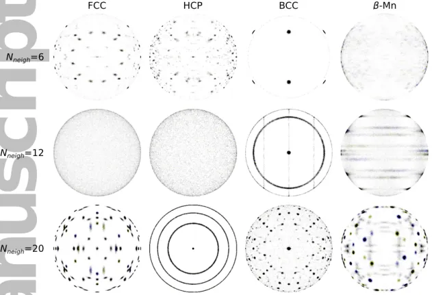
Crystal structures can be visualized in the same manner as BOODs29,30,28,10 _using

his-tograms of the bonds between neighboring particles, rotated into the reference frame of the

local neighborhood as defined above. This procedure forms distinct patterns — much like

BOODs — for different structures and numbers of neighbors. For several ideal structures with Gaussian noise applied to the positions, we show histograms on the surface of a unit sphere of the four nearest neighbor bonds in this reference frame in Figure 3 below.

To create a numerical description of neighboring particle bonds, we use sets of spherical

harmonicsYm

l (θ, ϕ), which are a natural set of basis functions for density maps — like these local

BOODs — on the surface of a sphere. Because our definition above creates a useful orientation for each particle based on its local environment, we do not have to resort to using

rotation-invariant combinations of spherical harmonics17 _{and can evaluate the spherical harmonics for}

alllandm.

We can reduce the spherical harmonics in a number of ways based on the desired application and the capacity of the machine learning methods we plan to use. When classifying individual

particles, we use the neighbor-averaged spherical harmonics: for each particle i and a set of

spherical harmonics of degreel and orderm, we define

¯ Y_lm(i, Nn) = 1 Nn Nn ∑ j=1 Y_lm(θij, ϕij) (1)

whereθij and ϕij are the spherical coordinates of the bond from particle ito particlej in the

reference frame of the local neighborhood of particlei as defined above and Nn is the number

of nearest-neighbor bonds to consider. This averaging method is the same idea that is used

Author Manuscript

harmonics would constructively interfere at particular frequencies (here particular orders of

spherical harmonics (l, m) would exhibit constructive interference for particular patterns, such

as the eight vertices of an axis-aligned cube), while others would exhibit only noise.

We find that neighbor-averaged spherical harmonics work well in a supervised ML setting, but due to the combinatorial degeneracy of placing particles inside neighbor shells, the neighbor-averaged spherical harmonics do not work as well for unsupervised learning algorithms. When training unsupervised models, we can instead look at globally-averaged spherical harmonics:

that is, for a particularl andm, we generate

¯ ¯ Y_lm= 1 NpNn Np ∑ i=1 Nn ∑ j=1 Y_lm(θij, ϕij) (2)

where Np is the number of particles in the system. This is equivalent to taking the spherical

harmonic transformation of the local BOODs shown in Figure 3. This method sacrifices some of the convenient locality properties of the neighborhood orientation: if there are grain boundaries or defects in the system, their signal will be reflected in the description of the whole system rather than being localized to the particles that are part of the grain boundary or defect.

Using Spherical Harmonic Descriptors for Structure

Iden-tification

To validate the usefulness of our local neighborhood spherical harmonic descriptors, we study

the simulation results of a paper11_{describing the assembly behavior of a host of complex crystal}

structures, including clathrates and quasicrystals. We chose this study because it contains some of the most complex crystals in terms of size and structure of the repeat unit that have been

predicted so farvia colloidal and nanoscale self-assembly. The crystals were all obtained using

the same two-parameter pair potential, defined as follows:

V(r) = 1

r15 +

1

r3cos (k(r−1.25)−ϕ).

The potential was truncated, shifted, and smoothed to zero at the third maximum to create short-range interaction potentials. The systems were slowly cooled to a low temperature from thermalized initial conditions, creating minimal surface area droplets (not connected through periodic boundary conditions) and columns (connected through periodic boundary conditions

Author Manuscript

in one dimension) of solid. Different combinations of the two independent potential

parame-ters k and ϕproduced different crystal structures. Including statistical replicas, this data set

contains over 1,100 samples — a volume that would take a researcher performing manual anal-ysis days or weeks to identify. Below we show that by using the spherical harmonics of the

neighbor bond distribution — oriented via the local environment — coupled to standard

ma-chine learning methods, we are able to analyze this data set, withouta priori knowledge of the

structures, in an automated manner in under 30 minutes on a common desktop processor. We

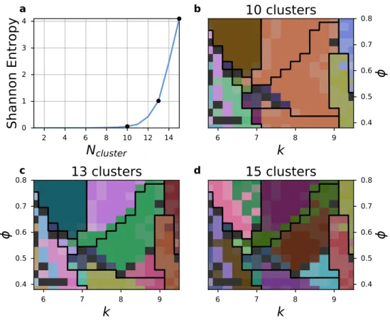
first pair our descriptors with an unsupervised ML method (clustering via Gaussian Mixture

Models32) to identify interesting structural regions of phase space and then with a supervised

ML algorithm (artificial neural networks) to generate a complete phase diagram from exemplar crystal structures. Detailed descriptions of the analysis performed in all cases are available in the Supplementary Information.

Unsupervised Learning

After generating the data, analysis of simulation results typically begins by trying to determine which — if any — crystal structures are present, with the eventual goal of identifying distinct regions in parameter space where each structure is formed. A simulation dataset could include thousands of combinations of simulation parameters and several replicas for each condition, so being able to lump together similar structures in an automated manner can reduce the required human work by orders of magnitude. This stage of analysis is an ideal application of unsupervised learning, which is often used to group data points together based on some idea of similarity in a high-dimensional space.

We use Gaussian mixture models (GMMs) as implemented in scikit-learn33 _{to perform}

un-supervised learning. Briefly, GMMs attempt to create a probability density function that agrees well with the distribution of observed data by using a given number of Gaussian functions in the input space. The number of Gaussian components in the mixture model is typically found

by optimizing the Bayesian information criterion (BIC)34, which measures how well a GMM fits

the observed data while penalizing models with many parameters to prevent overfitting. While GMMs produced by optimizing the BIC usually fit well the density distribution of the dataset they are trained on, the clusters that underlie our data are very commonly not Gaussian-distributed in space. This means that a mapping from the Gaussian component to which a point belongs (or the vector of probabilities for each component) to more meaningful

Author Manuscript

cluster membership is necessary. Several algorithms based on various strategies for generating

such a mapping have been proposed over the years35,36,37,38. In this work we use the method of

Baudry36_{, which greedily merges pairs of components based on the largest decrease in Shannon}

entropy (for observationsi and componentsj, −∑

i,j

pi,jln(pi,j)) caused by merging the pair of

components.

Because there are over one thousand simulated systems in the icosahedral quasicrystal

dataset11_{, we use globally-averaged spherical harmonics instead of neighborhood-averaged}

spher-ical harmonics for our GMMs, as in Equation 2. To find appropriate values for the maximum number of neighbors we use for the local bond descriptors and an appropriate maximum

spher-ical harmonic degreel for the local environment descriptors, we simultaneously optimize these

values and the number of Gaussian components in the mixture model using the BIC after

pro-jecting the descriptors to 128 dimensions using Principal Component Analysis (PCA)39 if the

number of descriptors for each system is greater than 128. In this way we choose a set of de-scriptors that is most readily fit by Gaussian mixtures with the fewest tunable parameters. To improve the reproducibility of the GMM fits to the observed probability distributions, we also select the best GMM (as judged by the BIC) out of three different initial configurations for each parameter set. In the end, this procedure selects 7 maximum nearest neighbors, a max-imum spherical harmonic degree of 7, and a GMM of 15 Gaussian components. In summary, the globally-averaged spherical harmonics produce a vector of spherical harmonics of length 36

(corresponding to the eighth triangle numberT8: we produce spherical harmonics with 0< l≤7

and 0≤m≤l) for each number of nearest neighborsNn ∈[4,7], which we concatenate into one

vector of length 140 for each system snapshot after excluding the constant ¯Y¯00. We use PCA

to project the input data into 128 dimensional space before formulating GMMs. We note that the final unsupervised learning results (after merging GMM components) are qualitatively very similar for all combinations of these parameters we tried for less than one close-packed neighbor

shell (around 12 neighbors) and with moderate-to-low spherical harmonic degree (lmax≤12).

After finding a GMM that fits the data well, we can merge Gaussian mixture components

to identify the clusters found in our data. Following the method of Baudry36, we sequentially

merge pairs of GMM components that yield the largest decrease in Shannon entropy. Figure 4(a) shows the Shannon entropy as GMM components are merged from the original 15 clusters — where each cluster corresponds to a GMM component — down to 1 cluster. In general for this method, the correct number of clusters to use is indicated by an upward elbow in the entropy

Author Manuscript

plot. For data that are not perfectly Gaussian in nature, however, the elbow is smoothed out into more of a curve. Based on this analysis, reasonable choices for the number of clusters to select may be between 9 and 13.

Phase diagrams for three selections of cluster counts, colored by the clusters found at each point in parameter space, are shown in Figure 4(b-d). Of the structures in this dataset, we find that the models are able to distinguish least clearly between the high-density icosahedral quasicrystal approximant and the disordered region as these are the first components to be merged. In general, we would expect cleaner crystals and crystals with fewer local environments to have more distinct spherical harmonic signatures that are easier for the GMMs to distinguish. Even without knowing how many phases are contained within, the model very accurately maps out the areas associated with the five crystalline regions, the icosahedral/quasicrystal region, and the disordered region. By clustering similar samples together, unsupervised learning can reduce the number of structures in this dataset that must be identified by an expert from over 1,100 to the order of a dozen. Here it is important to note that the results of unsupervised learning still require manual analysis in order to identify the structures present within the phase diagram, for example by manually identifying the best-scored sample for each cluster; once this step has been completed, these exemplar structures can be used to formulate a supervised learning classifier for high-throughput identification of structures as illustrated in the next section.

One interesting observation is the presence of multiple predicted phases in the cP8 and

hP2 regions of the phase diagram. As shown in Figure 5, on closer inspection we find that

one of the cP8 region structures of the original study11 _{corresponds to a cP8 structure and}

the others indicate polycrystalline cP8 and mixed systems ofcP8 andtP30 (Frank-Kasperσ)

phases. To identify individual particles or crystalline domains as thecP8 or tP30 phases, we

could apply supervised learning to the descriptors of individual particles’ local environments

instead of globally averaging the descriptors over entire systems. In contrast to thecP8 case,

the two types of structures found in thehP2 region correspond to a more- and less-well ordered

version of the same hP2 crystal. Because these structures are so similar, it makes sense that

they are among the earliest sets of GMM components to be merged. To qualitatively compare

Author Manuscript

Supervised Learning

With supervised learning methods, we can use our local environment descriptors to create order parameters based on our knowledge of which structures are present in the systems we study. We take exemplary simulation data for the five periodic crystal structures, the low- and medium-density icosahedral quasicrystals, the high-medium-density periodic quasicrystal approximant structure,

and four points in the disordered region of the phase diagram from manual analysis11_{and train a}

simple feedforward artificial neural network2_{(ANN) with one hidden layer to predict the}

struc-ture (i.e., from which exemplar sample each particle was taken) from the neighbor-averaged

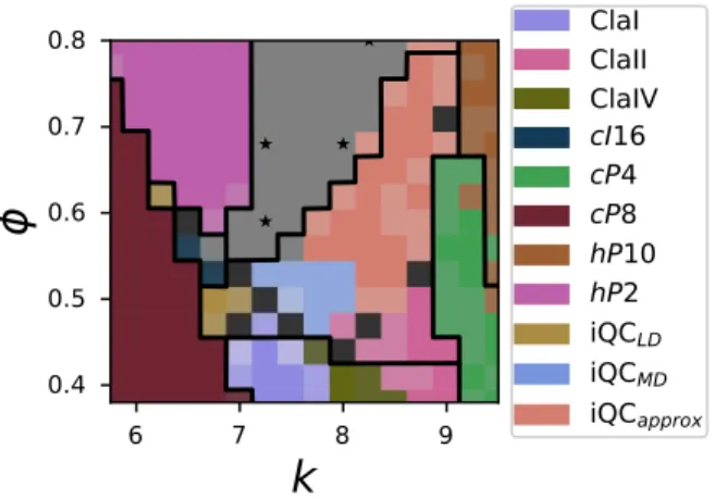
spherical harmonics of each particle, as given in Equation 1. As in our unsupervised learning example, we use local environments from 4–7 nearest neighbors and a maximum spherical har-monic degree of 7 to generate a 140-dimensional input vector for each particle. We use this ANN to construct the phase diagram by finding the most common particle type prediction among all particles in the systems at a particular set of conditions. The phase diagram colored by the most prevalent predicted structure in each simulation is shown in Figure 6.

Although there are still sometP30 samples in thecP8 region of the phase diagram, the ANN

identifies the whole region as entirely cP8 because tP30 was not given as a distinct example

structure for training. This makes sense because cP8 and tP30 are similar structures, so the

ANN identifies thetP30 samples as the nearest structure in descriptor space that it was trained

on — that is,cP8. This ability togeneralizewith sensible responses to previously-unseen data is

strongly influenced by the choice of descriptors and ML model and cannot be taken for granted, as illustrated by the comparison to Steinhardt order parameters below.

In the original study11_{, detailed analysis of the clathrate region of the phase diagram was}

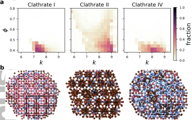
omitted, partly because the clathrates are complicated structures which often appear next to each other in the same simulation to form mixtures. Because the ANN provides a structure estimate for each particle in a system, we can use it to quantitatively identify the prevalence of the three clathrate structures present in this phase diagram, as shown in Figure 7(a). The ANN

finds an abundance of clathrate I at lowk, II at highk, and IV at intermediatek, just as was

qualitatively described in the original study.

Our supervised learning model can also be used to help isolate individual grains within a sample, or one structure from another in a mixed system. In Figure 7(b), we show a few typical systems of clathrates, with each particle colored according to its predicted type based on its

2

Author Manuscript

local environment. Visually, the ANN is able to distinguish the square tiling arrangement of cage motifs found in clathrate I from the rhombic and triangular arrangement of cage motifs found in clathrates II and IV, even in highly mixed systems.

Comparison to Steinhardt Order Parameters

We compare our local spherical harmonic descriptors to the Steinhardt order parameters — which are among the simplest comparable methods and have been extensively used in analysis

of 3D ordered systems17,18,19,20— to get an idea of their capability. In general, there are many

factors that should be carefully considered when comparing two sets of descriptors. Desirable attributes include low computational complexity, high information density, and the ability to be

inverted (i.e., to easily compute a structure from a set of descriptor values) or refined (i.e., to

be able to generate successively higher-fidelity descriptions). For the purpose of comparing to previous work, here we will focus more concretely on the performance of descriptors in supervised learning applications.

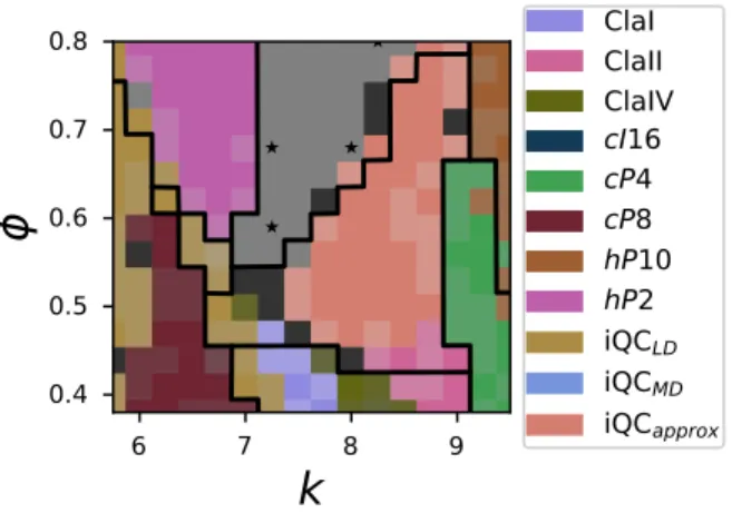
To probe the difference between our neighbor-averaged spherical harmonic descriptors to the Steinhardt order parameters, we generate a phase diagram of the icosahedral quasicrystal dataset using an ANN trained on a vector of per-particle Steinhardt order parameters for particle

i,Ql(i) (withl from 2 to 20): Ql(i) = 1 Nn v u u u t 4π 2l+ 1 l ∑ m=₋l N∑n(i) j=1 Ym l (θij, ϕij) 2 . (3)

Here we take the neighbors that we sum over as all particles within two standard deviations of the first four nearest-neighbor distances over the whole sample. While this is potentially a somewhat simplistic choice and more sophisticated methods of using Steinhardt order parameters have

been explored20_{, this is effective to illustrate a baseline comparison of the Steinhardt order}

parameters and our local environment spherical harmonic descriptors. The Steinhardt order parameter phase diagram should be directly comparable to the phase diagram generated using neighbor-averaged spherical harmonics in Figure 6. We show the supervised learning phase diagram generated from Steinhardt order parameter descriptors in Figure 8.

We find that, while the phase diagram generated from Steinhardt order parameters agrees with manual analysis in most cases, it differs significantly in how well the ANN model can

Author Manuscript

that the network trained with Steinhardt order parameters identifies tP30, mixed cP8-tP30,

and even pure cP8 systems in the high ϕ region as the low-density icosahedral quasicrystal

structure. Overall, the local environment spherical harmonics seem to generalize better in this case for the purpose of identifying structures than the Steinhardt order parameters.

Conclusion

We have introduced a generalized structural descriptor of a particle’s local environment that is sensitive to the symmetry of the local neighborhood. These descriptors are scale-free and rotation-invariant, and are useful for supervised, as well as unsupervised, learning of ordered systems. By coupling our numerical descriptions of local environments to common, readily-available machine learning algorithms, we are able to locate interesting structural regions of a complex phase diagram without prior information or to apply our knowledge of the available structures to generate phase diagrams automatically. Because the rate-limiting step of clustering observations into sets of distinct structures happens in an unsupervised manner, this method is highly useful for analyzing results of high-throughput computational experiments. Even though the descriptors are relatively short-ranged, only looking at the 7 nearest neighbors of each particle in this case, they are able to distinguish complicated clathrate structures with dozens of particles in a unit cell — and even an icosahedral quasicrystal that has no unit cell, but possesses extraordinarily complex orientational order.

In summary, our method allows machine learning algorithms to automatically build order parameters that describe interesting structural behavior from data sets. The machine learning methods and structural descriptors are applicable anywhere that the local environment of a system needs to be characterized, even for complex crystals. We expect our method to be useful in the study of crystal nucleation and growth, glass behavior, and building block design for engineering desirable structures.

Acknowledgments

This contribution was identified by Andrew Ferguson (University of Illinois at Urbana-Champaign) as the Best Presentation in the session “Data Mining and Machine Learning in Molecular Sci-ences I” of the 2016 AIChE Annual Meeting in San Francisco. The authors thank Julia Dshe-muchadse for helpful discussion of symmetry and structure. M. S. acknowledges support from

Author Manuscript

the University of Michigan Rackham Predoctoral Fellowship program. S. C. G. was partially supported by a Simons Investigator award from the Simons Foundation. Toyota Research In-stitute (“TRI”) provided funds to assist the authors with their research but this article solely reflects the opinions and conclusions of its authors and not TRI or any other Toyota entity.

Literature Cited

1. Henzie J, Gr¨unwald M, Widmer-Cooper A, Geissler PL, Yang P. Self-assembly of

uni-form polyhedral silver nanocrystals into densest packings and exotic superlattices. Nature

Materials 2012;11(2):131–137.

2. Shevchenko EV, Talapin DV, Kotov NA, O’Brien S, Murray CB. Structural diversity in

bi-nary nanoparticle superlattices. Nature 2006;439(7072):55–59. doi:10.1038/nature04414.

3. Macfarlane RJ, Lee B, Jones MR, Harris N, Schatz GC, Mirkin CA. Nanoparticle

super-lattice engineering with DNA. Science 2011;334(6053):204–208.

4. Zhang C, Macfarlane RJ, Young KL, Choi CHJ, Hao L, Auyeung E, Liu G, Zhou X,

Mirkin CA. A general approach to DNA-programmable atom equivalents.Nature Materials

2013;12(8):741–746.

5. Li B, Zhou D, Han Y. Assembly and phase transitions of colloidal crystals.Nature Reviews

Materials 2016;1:15011.

6. Hynninen AP, Christova CG, van Roij R, van Blaaderen A, Dijkstra M. Prediction and

observation of crystal structures of oppositely charged colloids. Physical Review Letters

2006;96(13). doi:10.1103/PhysRevLett.96.138308.

7. Glaser MA, Grason GM, Kamien RD, Koˇsmrlj A, Santangelo CD, Ziherl P.

Soft spheres make more mesophases. Europhysics Letters (EPL) 2007;78(4):46004.

doi:10.1209/0295-5075/78/46004.

8. Batten RD, Huse DA, Stillinger FH, Torquato S. Novel ground-state crystals with

con-trolled vacancy concentrations: from kagom´e to honeycomb to stripes. Soft Matter

Author Manuscript

9. Costa Campos LQ, de Souza Silva CC, Apolinario SWS. Structural phases

of colloids interacting via a flat-well potential. Physical Review E 2012;86(5).

doi:10.1103/PhysRevE.86.051402.

10. Damasceno PF, Engel M, Glotzer SC. Predictive self-assembly of polyhedra into complex

structures. Science 2012;337(6093):453–457.

11. Engel M, Damasceno PF, Phillips CL, Glotzer SC. Computational self-assembly of a

one-component icosahedral quasicrystal. Nature Materials 2015;14(1):109–116.

12. Bernard EP, Krauth W. Two-step melting in two dimensions:

first-order liquid-hexatic transition. Physical Review Letters 2011;107(15):155704.

doi:10.1103/PhysRevLett.107.155704.

13. Engel M, Anderson JA, Glotzer SC, Isobe M, Bernard EP, Krauth W. Hard-disk equation of state: first-order liquid-hexatic transition in two dimensions with three simulation methods.

Physical Review E 2013;87(4). doi:10.1103/PhysRevE.87.042134.

14. Wojciechowski KW, Frenkel D. Tetratic phase in the planar hard square

sys-tem? Computational Methods in Science and Technology 2004;10(2):235–255. doi:10.12921/cmst.2004.10.02.235-255.

15. Donev A, Burton J, Stillinger FH, Torquato S. Tetratic order in the phase

behavior of a hard-rectangle system. Physical Review B 2006;73(5):054109.

doi:10.1103/PhysRevB.73.054109.

16. Redner GS, Hagan MF, Baskaran A. Structure and dynamics of a

phase-separating active colloidal fluid. Physical Review Letters 2013;110(5):55701.

doi:10.1103/PhysRevLett.110.055701.

17. Steinhardt PJ, Nelson DR, Ronchetti M. Bond-orientational order in liquids and glasses.

Physical Review B 1983;28(2):784.

18. van Duijneveldt JS, Frenkel D. Computer simulation study of free energy

barri-ers in crystal nucleation. The Journal of Chemical Physics 1992;96(6):4655–4668.

Author Manuscript

19. Yan Z, Buldyrev SV, Giovambattista N, Stanley HE. Structural order for

one-scale and two-scale potentials. Physical Review Letters 2005;95(13):130604.

doi:10.1103/PhysRevLett.95.130604.

20. Lechner W, Dellago C. Accurate determination of crystal structures based on averaged

local bond order parameters. The Journal of Chemical Physics 2008;129(11):114707.

doi:10.1063/1.2977970.

21. Wolde PRt, Ruiz-Montero MJ, Frenkel D. Numerical calculation of the rate of crystal

nucleation in a Lennard-Jones system at moderate undercooling. The Journal of Chemical

Physics 1996;104(24):9932–9947. doi:10.1063/1.471721.

22. Chau PL, Hardwick AJ. A new order parameter for tetrahedral configurations. Molecular

Physics 1998;93(3):511–518. doi:10.1080/002689798169195.

23. Haji-Akbari A, Engel M, Keys AS, Zheng X, Petschek RG, Palffy-Muhoray P, Glotzer SC.

Disordered, quasicrystalline and crystalline phases of densely packed tetrahedra. Nature

2009;462(7274):773–777. doi:10.1038/nature08641.

24. Phillips CL, Voth GA. Discovering crystals using shape matching and machine learning.

Soft Matter 2013;9(35):8552–8568.

25. Reinhart WF, Long AW, Howard MP, Ferguson AL, Panagiotopoulos AZ. Machine learning

for autonomous crystal structure identification.Soft Matter2017;doi:10.1039/C7SM00957G.

26. Dietz C, Kretz T, Thoma MH. Machine-learning approach for local classification of

crystalline structures in multiphase systems. Physical Review E 2017;96(1):011301.

doi:10.1103/PhysRevE.96.011301.

27. Cubuk ED, Schoenholz SS, Rieser JM, Malone BD, Rottler J, Durian DJ, Kaxiras E, Liu AJ. Identifying structural flow defects in disordered solids using machine-learning methods.

Physical Review Letters 2015;114:108001. doi:10.1103/PhysRevLett.114.108001. 28. Keys AS, Iacovella CR, Glotzer SC. Characterizing structure through shape matching and

applications to self-assembly. Annual Review of Condensed Matter Physics 2011;2(1):263–

Author Manuscript

29. Dzugutov M. Formation of a dodecagonal quasicrystalline phase in a simple monatomic

liquid. Physical Review Letters 1993;70:2924–2927. doi:10.1103/PhysRevLett.70.2924.

30. Roth J, Denton AR. Solid-phase structures of the Dzugutov pair potential.Physical Review

E 2000;61(6):6845–6857. doi:10.1103/PhysRevE.61.6845.

31. Seo D, Yoo CI, Chung IS, Park SM, Ryu S, Song H. Shape adjustment between mul-tiply twinned and single-crystalline polyhedral gold nanocrystals: decahedra, icosahedra,

and truncated tetrahedra. The Journal of Physical Chemistry C 2008;112(7):2469–2475.

doi:10.1021/jp7109498.

32. Dempster AP, Laird NM, Rubin DB. Maximum likelihood from incomplete data via the EM

algorithm. Journal of the Royal Statistical Society Series B (Methodological) 1977;39(1):1–

38.

33. Pedregosa F, Varoquaux G, Gramfort A, Michel V, Thirion B, Grisel O, Blondel M, Pret-tenhofer P, Weiss R, Dubourg V, Vanderplas J, Passos A, Cournapeau D, Brucher M,

Perrot M, Duchesnay E. Scikit-learn: machine learning in Python. Journal of Machine

Learning Research 2011;12:2825–2830.

34. Schwarz G. Estimating the dimension of a model. The Annals of Statistics 1978;6(2):461–

464. doi:10.1214/aos/1176344136.

35. Hennig C. Methods for merging Gaussian mixture components.Advances in Data Analysis

and Classification 2010;4(1):3–34. doi:10.1007/s11634-010-0058-3.

36. Baudry JP, Raftery AE, Celeux G, Lo K, Gottardo R. Combining mixture components for

clustering. Journal of Computational and Graphical Statistics 2010;19(2):332–353.

37. Pastore A, Tonellato S. A merging algorithm for Gaussian mixture components. Working Paper 2013:04; Department of Economics, University of Venice “Ca’ Foscari”; 2013.

38. Scrucca L. Identifying connected components in Gaussian finite mixture

mod-els for clustering. Computational Statistics & Data Analysis 2016;93:5–17.

doi:10.1016/j.csda.2015.01.006.

39. Pearson K. On lines and planes of closest fit to systems of points in space. The London,

Author Manuscript

40. Chollet F. Keras. 2015.

List of Figures

1. Key results from a self-assembly study of isotropic pair potentials11. (a) The oscillating

pair potentialV(r) used in the study and a schematic adaptation of the phase diagram11_as

generated by manual analysis of the structures generated by systematically varyingkand

ϕ. The quasicrystalline region contains low-density and intermediate-density icosahedral

quasicrystals, as well as a high-density quasicrystal approximant. The clathrates that form are typically a mixture of clathrates I, II, and IV, with the prevalence of individual

structures primarily dictated by the potential parameter k. (b) A subset of the simple

and complex structures that self-assemble from the oscillating pair potential. For each structure, Pearson symbols and particle configurations in crystal unit cells are shown on the left, and Voronoi polyhedra corresponding to representative nearest-neighbor local environments are shown on the right.

2. Bond orientational order diagrams (BOODs) for various systems. (a) Geometry schemat-ics and BOODs for simple cubic, body-centered cubic, and face-centered cubic structures. (b) Geometry schematics and BOODs of structures with multiple local environment ori-entations. The BOOD is the superposition of the signals from the bonds of each local environment orientation. (c) BOODs of real face-centered cubic structures with defects. Above, the BOOD appears very similar to that of a hexagonally close-packed structure due to stacking faults. Below, the BOOD appears to exhibit 10-fold symmetry due to polycrystallinity. Points with blue and yellow coronas are only on the front-facing and back-facing side of the sphere, respectively.

3. Sphere surface histogram of four nearest-neighbor bonds in the local reference frame as defined by the nearest 6, 12, and 20 neighbors for face-centered cubic, hexagonally

close-packed, body-centered cubic andβ-manganese structures. FCC and HCP have full

neigh-bor shells at 12 neighneigh-bors with diagonal or nearly-diagonal inertia tensors, so they mostly

exhibit noise. β-manganese is a more complex structure with 20 particles per unit cell and

exhibits weak patterns at low neighbor counts for this amount of noise.

4. Icosahedral quasicrystal dataset phase diagrams generated by unsupervised Gaussian Mix-ture Models (GMMs). (a) Shannon entropy (blue line) of the quasicrystal dataset as GMM

Author Manuscript

components are successively merged from 15 clusters to one cluster. Merged cluster counts corresponding to (b-d) are indicated by black points. (b-d) Phase diagrams generated by taking the most common predicted cluster type for each parameter point, indicated by the black points in (a). For each selected cluster count, dark gray regions show a poor prefer-ence for any single structure among the samples for those parameters. Each type of system as identified by the GMM is assigned a different color, but this unsupervised algorithm clusters the distinct structures that it finds rather than labeling a previously-identified set

of known structures. Phase boundaries generated by manual analysis11 _{are included for}

reference as black lines.

5. Different crystal structures as identified by unsupervised learning of local environments. Colors correspond to the clusters identified by GMM components in Figure 4(d). (a-b)

Pure cP8 and mixed cP8−tP30 phases in the cP8 region of the phase diagram.

(c-d) More-ordered and less-ordered hP2 crystals, respectively. (e-f) BOODs of more- and

less-well-orderedhP2 crystals.

6. Supervised phase diagram generated by a neural network trained on representative struc-tures at particular points in parameter space. Stars indicate locations of training data for

the disordered region. Black lines are phase boundaries as identified by hand in11_.

7. Identification of clathrate local environments using supervised learning. (a) Fraction of particles in systems identified as clathrate I, II, and IV, as identified by an ANN. (b) Three representative snapshots of simulations with particles colored by their identified structure type and a few characteristic cage arrangements from each sample emphasized. Red: clathrate type I, brown: clathrate type II, blue: clathrate type IV.

8. Supervised phase diagram generated using a vector of per-particle Steinhardt order

Author Manuscript

Figure 1: Key results from a self-assembly study of isotropic pair potentials

. (a) The

oscillat-ing pair potential

V

(

r

) used in the study and a schematic adaptation of the phase diagram

as

generated by manual analysis of the structures generated by systematically varying

k

and

ϕ

. The

quasicrystalline region contains low-density and intermediate-density icosahedral quasicrystals, as

well as a high-density quasicrystal approximant. The clathrates that form are typically a mixture

of clathrates I, II, and IV, with the prevalence of individual structures primarily dictated by the

potential parameter

k

. (b) A subset of the simple and complex structures that self-assemble from

the oscillating pair potential. For each structure, Pearson symbols and particle configurations in

crystal unit cells are shown on the left, and Voronoi polyhedra corresponding to representative

nearest-neighbor local environments are shown on the right.

Author Manuscript

Figure 2: Bond orientational order diagrams (BOODs) for various systems. (a) Geometry

schemat-ics and BOODs for simple cubic, body-centered cubic, and face-centered cubic structures. (b)

Ge-ometry schematics and BOODs of structures with multiple local environment orientations. The

BOOD is the superposition of the signals from the bonds of each local environment orientation. (c)

BOODs of real face-centered cubic structures with defects. Above, the BOOD appears very similar

to that of a hexagonally close-packed structure due to stacking faults. Below, the BOOD appears

to exhibit 10-fold symmetry due to polycrystallinity. Points with blue and yellow coronas are only

on the front-facing and back-facing side of the sphere, respectively.

Author Manuscript

Figure 3: Sphere surface histogram of four nearest-neighbor bonds in the local reference frame as

defined by the nearest 6, 12, and 20 neighbors for face-centered cubic, hexagonally close-packed,

body-centered cubic and

β

-manganese structures.

FCC and HCP have full neighbor shells at

12 neighbors with diagonal or nearly-diagonal inertia tensors, so they mostly exhibit noise.

β

-manganese is a more complex structure with 20 particles per unit cell and exhibits weak patterns

at low neighbor counts for this amount of noise.

Author Manuscript

N

Shannon Entropy

k

ϕ

10 clusters

k

ϕ

13 clusters

k

ϕ

15 clusters

Figure 4: Icosahedral quasicrystal dataset phase diagrams generated by unsupervised Gaussian

Mixture Models (GMMs). (a) Shannon entropy (blue line) of the quasicrystal dataset as GMM

components are successively merged from 15 clusters to one cluster. Merged cluster counts

cor-responding to (b-d) are indicated by black points. (b-d) Phase diagrams generated by taking the

most common predicted cluster type for each parameter point, indicated by the black points in (a).

For each selected cluster count, dark gray regions show a poor preference for any single structure

among the samples for those parameters. Each type of system as identified by the GMM is

as-signed a different color, but this unsupervised algorithm clusters the distinct structures that it finds

rather than labeling a previously-identified set of known structures. Phase boundaries generated

by manual analysis

are included for reference as black lines.

Author Manuscript

Figure 5: Different crystal structures as identified by unsupervised learning of local environments.

Colors correspond to the clusters identified by GMM components in Figure 4(d). (a-b) Pure

cP

8

and mixed

cP

8

−

tP

30 phases in the

cP

8 region of the phase diagram. (c-d) More-ordered and

less-ordered

hP

2 crystals, respectively. (e-f) BOODs of more- and less-well-ordered

hP

2 crystals.

Author Manuscript

k

ϕ

Figure 6: Supervised phase diagram generated by a neural network trained on representative

struc-tures at particular points in parameter space. Stars indicate locations of training data for the

disordered region. Black lines are phase boundaries as identified by hand in

.

Author Manuscript

Figure 7: Identification of clathrate local environments using supervised learning. (a) Fraction

of particles in systems identified as clathrate I, II, and IV, as identified by an ANN. (b) Three

representative snapshots of simulations with particles colored by their identified structure type and

a few characteristic cage arrangements from each sample emphasized. Red: clathrate type I, brown:

clathrate type II, blue: clathrate type IV.

Author Manuscript

k

ϕ

Figure 8: Supervised phase diagram generated using a vector of per-particle Steinhardt order

parameters ¯

Q

.