Ann. Geophys., 26, 1439–1449, 2008 www.ann-geophys.net/26/1439/2008/ © European Geosciences Union 2008
Annales
Geophysicae
Statistical study of inverted-V structures in FAST data
N. Partamies1, E. Donovan2, and D. Knudsen2
1Finnish Meteorological Institute, Helsinki, Finland
2Institute for Space Research, University of Calgary, Calgary, Canada
Received: 8 January 2008 – Revised: 21 March 2008 – Accepted: 16 April 2008 – Published: 11 June 2008
Abstract. Since the 1970s the inverted-V structures have
been observed in the satellite-borne particle data. These3 -shaped enhancements of the differential energy flux on the high energy channels on the top of low number flux on the lower energies are traces of auroral particle acceleration by U-shaped potential drops along the field lines within the au-roral zones. In this study, we show the results of a statistical study of inverted-V events in five years (1997–2001) of the Fast Auroral SnapshoT (FAST) electron spectrograms. We found 588 well-defined events in total, but the statistical re-sults are also shown for a subset of 97 very best events.
The statistical analysis shows that the inverted-V’s mainly occur within the auroral oval latitudes (65◦–75◦ invariant latitude), in the pre-midnight sector (21–23 magnetic local time) and during the Northern Hemisphere winter months (November to February). The typical maximum energies of the inverted-V’s are 2–4 keV, when a threshold value of 0.3 keV is used as a selection criterion. This corresponds to an acceleration potential drop of a few kV. The typical peak energy tends to increase towards the magnetic mid-night. Most of the inverted-V events occur during magnet-ically quiet or moderate activity,Kp 1–4. The usual width of an inverted-V varies from 20 to 40 km and is comparable to the peak value of the typical meso-scale auroral arc width of 10–20 km. Furthermore, the polar cap potential values es-timated from the SuperDARN radar data are always at least three times larger than the inverted-V acceleration potential drop.
Keywords. Ionosphere (Auroral ionosphere; Electric fields
and currents; Particle acceleration)
Correspondence to: N. Partamies ([email protected])
1 Introduction
Energies from a few keV to tens of keVs within the discrete aurora indicate energization of the magnetospheric particles before they precipitate into the ionosphere. Signatures of the particle acceleration can be seen in the satellite data. Prob-ably the most referred one is the inverted-V, a signature of particle acceleration in a U-shaped potential drop above the auroral arcs. Similar to the arcs, the inverted-V’s are thought to be elongated in the east-west direction (along the oval), although the direct measurements by polar orbiting satellites are always meridional cross-sections. At the bottom of the potential drop a field-aligned electric field accelerates elec-trons towards the ionosphere and ions out of the ionosphere resulting in an upward field-aligned current (FAC). The rela-tion between field-aligned currentj|| and the potential drop
V can be described by the equationj||=K(V+TE/e)(e.g. Janhunen, 1999), whereKis an experimental parameter, of-ten referred to as the field-aligned conductance, TE is the electron temperature in the source region, andeis the elec-tron charge. Olsson and Janhunen (2000) demonstrated that the linear relationship between FAC and the acceleration po-tential drop does not apply nearly as often as was believed in the past, but in most cases the current density is rather inde-pendent of the potential. In addition to a quasi-static potential drop, particles can be accelerated by wave-particle interac-tion, which may also act together with the DC potential drop. The nature of the actual acceleration process, however, is be-yond the scope of this paper. The potential structures that ac-celerate electrons downward and ions upward leave a cavity in the ionospheric plasma density. These cavities have been shown to exist at the altitudes of 2–6RE (Janhunen et al., 2002) above the auroral oval latitudes. Furthermore, the den-sity depletion regions have been suggested to act as a source for the auroral kilometric radiation (Strangeway et al., 2001). So, various interesting auroral phenomena are related, in one way or another, to the particle acceleration processes.
1440 N. Partamies et al.: Statistical study of inverted-V’s The very first report where the term inverted-V was used
was published in 1971 by Frank and Ackerson who described different electron acceleration events including an inverted-V. Based on a few events they concluded that inverted-V’s are substructures occurring during moderate magnetic activity with theKpindex ranging from 3 to 4+. They also found out that the maximum accelerated energy of these structures is of the order of a keV, and their typical duration in the energy-time spectrogram is 30–50 s, which corresponds to a distance of about 150–250 km. Bosqued et al. (1985) reported the first statistical study of about 250 inverted-V events as detected by the AUREOL-3 satellite. According to their results, the typical width of the V structures is 50–100 km and their peak energies are 1–5 keV. These findings suggested that most of the inverted-V’s are much wider than many narrow individ-ual auroral arcs (∼100 m, e.g. Borovsky, 1993) captured by high-resolution ground-based instruments. Instead of corre-sponding single arcs, most of the V-structures have been as-sociated with wider constellations of multiple arcs. However, smaller scale sizes, typically 28–35 km, and an exponential width distribution was reported by Newell et al. (1996).
Based on Defense Meteorological Satellite Program (DMSP) satellite data, an electron acceleration survey by Newell (2000) shows that only 4% of all of the acceleration events can be called V’s. Furthermore, the inverted-V’s may not be isolated but rather part of a larger accelera-tion structure. They classified all Large-Scale Acceleraaccelera-tion Events (LSAE) according to their shape in the spectrogram into seven different categories including e.g. flat electron sig-natures with a constant peak energy, monotonically increas-ing or decreasincreas-ing cases, which would correspond to S-shaped potential structures, inverted-V’s and forms that resemble inverted-V’s. The authors did not comment on the auroral displays corresponding to these different acceleration events. Individual electron spectra within an inverted-V typically has a single peak as a signature of acceleration. Most of these spectra are shown to fit well into an accelerated Maxwellian model spectrum (Olsson and Janhunen, 2000).
There are two main issues considered in this study. The first question is how closely the statistical appearance (i.e. their occurrence frequency as a function of MLT, ILAT, and other parameters) of the inverted-V’s can be related to that of the auroral arcs. Another question is whether a relationship can be found between the cross-polar cap potential and the particle acceleration potential above the auroral arcs. The rest of the paper is organised as follows: Sect. 2 describes the data and the event selection criteria, Sect. 3 contains the statistical results of our data set. Defining the widths of the inverted-V’s and their comparisons to the ones of the auroral arcs is explained in Sect. 4. Section 5 discusses the obser-vations and compares them both to the previous electron ac-celeration studies and to the related observations of other au-roral phenomena, such as strong ionospheric electric fields, average auroral intensity, upward ion beams, substorm oc-currence and plasma density cavities.
2 Event selection and data
We define an inverted-V as a3-shaped enhancement of the differential energy flux on the high energy channels on the top of low flux on the lower energies. We also require that the enhancement is strong enough – at least ten times higher than the simultaneous fluxes on the lower energy channels – and at high enough energies (at 300 eV or higher) to be easily distinguished from the possible secondary and thermal elec-tron fluxes of the background. The events were also required to be physically large enough, visible in at least three time steps, to form a3shape. Finally, we looked for symmetric events, whose peak position would not be more than three data points towards either end from the centre of the struc-ture. These requirements are based both on our experience and the previous work by Olsson and Janhunen (2000) and Newell (2000).
The particle detector on board the polar orbiting Fast Auroral SnapshoT (FAST) satellite (Carlson et al., 1998) records energies from 6 eV to 30 keV in 47 channels. The dif-ferential energy fluxes (in eV/m2s sr eV) are measured sep-arately for pitch angles of 0◦, 90◦ and 180◦. In this study,
we use all the data for 0◦pitch angle (precipitating) electrons from 1997–2001. FAST orbital period is about 133 min and thus, it makes about 11 orbits per day and 19 760 orbits in 5 years, which is half of the number of the available north-ern auroral oval crossings. The orbital altitude varies within about 400–4100 km and the average velocity of the satellite is about 6.9 km/s. In the FAST quicklook data, the average tem-poral resolution is about five seconds implying the minimum observable scale size (three time steps) to be about 70 km.
The altitudes of acceleration regions typically range from 1000 km to about 3RE(e.g. Gorney et al., 1981). Thus, some of the potential structures taking place around the lower end of this altitude range may be only partly recorded or missed by the FAST satellite, which sees only the part of the accel-erated precipitation that is located above the orbit.
From the five years worth of data we found 588 inverted-V events in total. An example of a typical inverted-inverted-V in the electron energy-time spectrogram is shown in Fig. 1. This event was observed on 7 May 1999 on the orbit number 10 713. It reached the peak energy of about 11 keV and it was observed by FAST for 35 s. This individual event was also examined in FAST high resolution data with the tem-poral resolution of 0.3 s, and it still showed up as a single, smooth inverted-V.
A subset of 97 excellent events was separated from the full data set. The distributions for all the basic parameters have been checked for both data sets to make sure that their behaviour is similar and thus, our definition of the inverted-V is strict enough.
The events that were rejected from our event set were typ-ically either not entirely visible due to the upper energy limit of the FAST particle sensor or missing data, highly asymmet-ric in peak position (by more than three data points towards
N. Partamies et al.: Statistical study of inverted-V’sPartamies et al.: Statistical Study of inverted-V’s 14413
8.46 8.47 8.48 8.49 8.5 8.51 8.52 8.53 8.54 1.0×100 1.0×101 1.0×10² 1.0×10³ 1.0×10⁴ 1.0×10⁵ UT Energy (keV) 1e+06 3.09e+07 6.09e+07 9.08e+07 1.21e+08 1.51e+08 1.81e+08 2.11e+08 2.41e+08 2.7e+08 3e+08 3.3e+08 3.6e+08 3.9e+08 4.2e+08 4.5e+08 4.8e+08 Diff. energy flux
Fig. 1. An example of an inverted-V in an electron spectrogram.
Colour coding shows the differential energy flux (eV/(cm2s sr eV)), and pink spots mark the V structure as defined from the data. Y-axis is energy and X-Y-axis can be given in latitude (GLAT, ILAT), universal time (UT) or magnetic local time (MLT). This event was observed on 7 May, 1999 on the orbit number 10713 at 08:27:36– 08:32:24 UT. FAST saw this inverted-V for about 35 seconds.
in Figure 2, we can examine the shape of the inverted-V’s. Averaging over all 97 curves gives the typical shape of these structures as seen in the spectrograms (thick line in Figure 2). The average curve forms a fairly symmetric and well-defined inverted-V with the peak energy of about 5 keV. Peak ener-gies of all of these events vary from a few keV up to 20 keV. The maximum seasonal occurrence of our events is in November to February, as can be seen from Figure 3, but there is another maximum (139 events) during the summer months from May to July. In this data set, there are only a few events from the southern hemisphere. The curve on the top of the distribution is reconstructed from satellite ob-servations of electron precipitation, according to Figure 2 by Barth et al. (2004). It shows the seasonal variation of the electron flux ratio of the northern and southern hemispheres. This to-south energy flux ratio is high when the north-ern hemisphere energy flux is high (northnorth-ern winter), and low when the electron precipitation in the southern hemisphere is strong (northern summer). The minimum of the flux ratio around the day number 172 (summer solstice) and the maxi-mum around the day number 355 (winter solstice) agree with the main features of the inverted-V occurrence, except the en-hancement in summer. On the other hand, the substorm oc-currence as studied by Wang and L¨uhr (2007) also has a
max-1 10 19
[image:3.595.315.545.63.387.2]0 10 20 Distance Energy (keV )
Fig. 2. Energy–distance curve of the best 97 events on the top of
each other. One of these curves comes from the pink spots in Fig-ure 1. The thickest line is an arithmetic average of all curves, i.e. an average shape of the inverted-V’s as seen in the electron data. No scaling has been done for these data.
imum in June in addition to the maximum in Dec–Feb. The seasonal maxima in the substorm and inverted-V occurrence coincide with lowest seasonal values of ionospheric Peder-sen conductivity. The only difference we found between the summer maximum events (May to Jul) and the events during the winter months (Nov to Feb) is that the majority of the winter events occur at lower latitudes (65–70◦ILAT), while the summer events are predominantly observed at higher lat-itudes (75–85◦ILAT).
The peak energy of the V-structures, i.e. the accelerated maximum energy at the top of theΛ-shape, is proportional to the acceleration potential drop. This energy value is typi-cally less than 6 keV (6 kV) as shown by Figure 4. This is in agreement with earlier results by e.g. Olsson et al. (1998), who stated that the potential drops related to auroral arcs range typically up to 5 kV, higher values being associated with the onset aurora and Westward Travelling Surge (WTS) type activity (up to 25 kV). Accelerated energies of 1–5 keV were already suggested by Bosqued et al. (1985). The num-ber of inverted-V’s decreases exponentially towards higher peak energies as shown by the curve fitted to the event num-bers of the full set (red solid line in Fig.4). This suggests that within the resolution limits of the observations, events with lower peak energies always occur more frequently. Notice that the first bin of the histogram is left out of the fit be-cause it is biased by the selection criterion that requires the peak energy to be greater than 0.3 keV. The satellite altitude may contribute to the observed peak energy if the orbit is too high and crosses the acceleration region so that only a part of
Fig. 1. An example of an inverted-V in an electron spectrogram.
Colour coding shows the differential energy flux (eV/(cm2s sr eV)), and pink spots mark the V structure as defined from the data. Y-axis is energy and X-Y-axis can be given in latitude (GLAT, ILAT), universal time (UT) or magnetic local time (MLT). This event was observed on 7 May 1999 on the orbit number 10 713 at 08:27:36– 08:32:24 UT. FAST saw this inverted-V for about 35 s.
either end), flat or monotonically increasing or decreasing, or had a shape of an upright V.
3 Statistical results
Extracting the maximum flux curve (as indicated by the pink crosses in Fig. 1) for each event and plotting these curves for the 97 best events on the top of each other, as shown in Fig. 2, we can examine the shape of the inverted-V’s. Averaging over all 97 curves gives the typical shape of these structures as seen in the spectrograms (thick line in Fig. 2). The average curve forms a fairly symmetric and well-defined inverted-V with the peak energy of about 5 keV. Peak energies of all of these events vary from a few keV up to 20 keV.
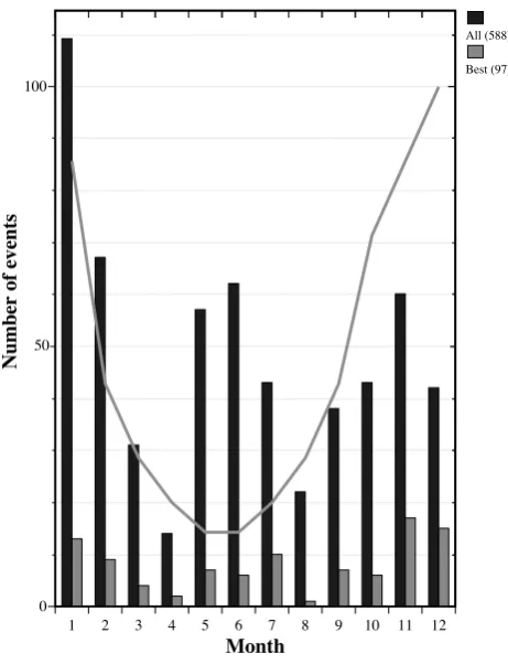
The maximum seasonal occurrence of our events is in November to February, as can be seen from Fig. 3, but there is another maximum (139 events) during the summer months from May to July. In this data set, there are only a few events from the Southern Hemisphere. The curve on the top of the distribution is reconstructed from satellite observa-tions of electron precipitation, according to Fig. 2 by Barth
Partamies et al.: Statistical Study of inverted-V’s
3
8.46 8.47 8.48 8.49 8.5 8.51 8.52 8.53 8.54
1.0×100 1.0×101 1.0×10² 1.0×10³ 1.0×10⁴ 1.0×10⁵
UT
Energy (keV)
1e+06 3.09e+07 6.09e+07 9.08e+07 1.21e+08 1.51e+08 1.81e+08 2.11e+08 2.41e+08 2.7e+08 3e+08 3.3e+08 3.6e+08 3.9e+08 4.2e+08 4.5e+08 4.8e+08 Diff. energy fluxFig. 1. An example of an inverted-V in an electron spectrogram.
Colour coding shows the differential energy flux (eV/(cm
2s sr eV)),
and pink spots mark the V structure as defined from the data.
Y-axis is energy and X-Y-axis can be given in latitude (GLAT, ILAT),
universal time (UT) or magnetic local time (MLT). This event was
observed on 7 May, 1999 on the orbit number 10713 at 08:27:36–
08:32:24 UT. FAST saw this inverted-V for about 35 seconds.
in Figure 2, we can examine the shape of the inverted-V’s.
Averaging over all 97 curves gives the typical shape of these
structures as seen in the spectrograms (thick line in Figure 2).
The average curve forms a fairly symmetric and well-defined
inverted-V with the peak energy of about 5 keV. Peak
ener-gies of all of these events vary from a few keV up to 20 keV.
The maximum seasonal occurrence of our events is in
November to February, as can be seen from Figure 3, but
there is another maximum (139 events) during the summer
months from May to July. In this data set, there are only
a few events from the southern hemisphere. The curve on
the top of the distribution is reconstructed from satellite
ob-servations of electron precipitation, according to Figure 2 by
Barth et al. (2004). It shows the seasonal variation of the
electron flux ratio of the northern and southern hemispheres.
This to-south energy flux ratio is high when the
north-ern hemisphere energy flux is high (northnorth-ern winter), and low
when the electron precipitation in the southern hemisphere is
strong (northern summer). The minimum of the flux ratio
around the day number 172 (summer solstice) and the
maxi-mum around the day number 355 (winter solstice) agree with
the main features of the inverted-V occurrence, except the
en-hancement in summer. On the other hand, the substorm
oc-currence as studied by Wang and L¨uhr (2007) also has a
max-1 10 19
[image:3.595.51.288.66.344.2]0 10 20 Distance Energy (keV )
Fig. 2. Energy–distance curve of the best 97 events on the top of
each other. One of these curves comes from the pink spots in
Fig-ure 1. The thickest line is an arithmetic average of all curves, i.e. an
average shape of the inverted-V’s as seen in the electron data. No
scaling has been done for these data.
imum in June in addition to the maximum in Dec–Feb. The
seasonal maxima in the substorm and inverted-V occurrence
coincide with lowest seasonal values of ionospheric
Peder-sen conductivity. The only difference we found between the
summer maximum events (May to Jul) and the events during
the winter months (Nov to Feb) is that the majority of the
winter events occur at lower latitudes (65–70
◦ILAT), while
the summer events are predominantly observed at higher
lat-itudes (75–85
◦ILAT).
The peak energy of the V-structures, i.e. the accelerated
maximum energy at the top of the
Λ-shape, is proportional
to the acceleration potential drop. This energy value is
typi-cally less than 6 keV (6 kV) as shown by Figure 4. This is in
agreement with earlier results by e.g. Olsson et al. (1998),
who stated that the potential drops related to auroral arcs
range typically up to 5 kV, higher values being associated
with the onset aurora and Westward Travelling Surge (WTS)
type activity (up to 25 kV). Accelerated energies of 1–5 keV
were already suggested by Bosqued et al. (1985). The
num-ber of inverted-V’s decreases exponentially towards higher
peak energies as shown by the curve fitted to the event
num-bers of the full set (red solid line in Fig.4). This suggests that
within the resolution limits of the observations, events with
lower peak energies always occur more frequently. Notice
that the first bin of the histogram is left out of the fit
be-cause it is biased by the selection criterion that requires the
peak energy to be greater than 0.3 keV. The satellite altitude
may contribute to the observed peak energy if the orbit is too
high and crosses the acceleration region so that only a part of
Fig. 2. Energy-distance curve of the best 97 events on the top of
each other. One of these curves comes from the pink spots in Fig. 1. The thickest line is an arithmetic average of all curves, i.e. an av-erage shape of the inverted-V’s as seen in the electron data. No scaling has been done for these data.
et al. (2004). It shows the seasonal variation of the elec-tron flux ratio of the Northern and Southern Hemispheres. This north-to-south energy flux ratio is high when the North-ern Hemisphere energy flux is high (northNorth-ern winter), and low when the electron precipitation in the Southern Hemi-sphere is strong (northern summer). The minimum of the flux ratio around the day number 172 (summer solstice) and the maximum around the day number 355 (winter solstice) agree with the main features of the inverted-V occurrence, except the enhancement in summer. On the other hand, the substorm occurrence as studied by Wang and L¨uhr (2007) also has a maximum in June in addition to the maximum in December–February. The seasonal maxima in the substorm and inverted-V occurrence coincide with lowest seasonal val-ues of ionospheric Pedersen conductivity. The only differ-ence we found between the summer maximum events (May to July) and the events during the winter months (November to February) is that the majority of the winter events occur at lower latitudes (65–70◦ILAT), while the summer events are predominantly observed at higher latitudes (75–85◦ILAT).
1442
4
N. Partamies et al.: Statistical study of inverted-V’sPartamies et al.: Statistical Study of inverted-V’s
1 2 3 4 5 6 7 8 9 10 11 12
0 100
Month
Number of events
All (588)
Best (97)
50
Fig. 3. Seasonal distribution of inverted-V events. Most events
are captured during the winter months, but another smaller popula-tion shows up during summer. The curve shows the seasonal varia-tion of the electron flux ratio of northern and southern hemispheres (Barth et al., 2004). Inverted-V events of this study have mainly been recorded over the norther auroral region.
the structure can be seen. In this case the peak energy would
have a tendency to decrease with an increasing altitude of the
orbit. Our survey of the FAST altitudes during the
inverted-V events (data not shown) revealed no correlation between
the peak energy and the spacecraft altitude. Thus, we
con-clude that our peak energy distribution is not biased by partly
recorded events.
Figure 5 shows that the peak energy grows towards the
Magnetic Local Time (MLT) midnight, where also the most
intense aurora occur. The highest peak energies appear at and
around 20–24 MLT and at and around 70 ILAT. The morning
sector in particular is dominated by low acceleration
ener-gies. Events at 80
◦ILAT or higher typically have low peak
energies as well as low energy flux values (<1mW/m
2). In
general, the highest energies appear at the times and places
where most of the inverted-V observations are found: around
21 MLT and 70–75
◦ILAT.
The Magnetic Local Time (MLT) distribution of the
inverted-V’s in Figure 6 shows that most of them take place
in the evening and pre-midnight sector around 21–23 MLT.
This behaviour agrees with that of the overall auroral
activ-ity. The MLT distribution in Figure 6 is normalised by the
time FAST spent in each MLT hour bin during the five years.
The overlaid curve is the occurrence of about 17,000
auro-ral arcs as a function of MLT (Syrj¨asuo and Donovan, 2004).
0 2 4 6 8 10 12 14 16 18 20
0 100
Peak energy (keV)
Number of events
All (588)
Best (97)
50
Fig. 4. The distribution of the peak energy observed within the
inverted-V’s. In most cases, the accelerated energies range from 2 to 4 keV. The overlaid red curve shows a fit of an exponential function into the whole data set.
The arc occurrence curve, too, has been normalised by the
total amount of ASC images taken in each MLT sector. The
striking similarity of these two distributions supports the idea
that the inverted-V’s are the type of acceleration of the
auro-ral arcs.
Kp index is a three-hour index of geomagnetic activity.
It is generated based on measurements at 12 or 13 stations
around the world, and its values range from 0 to 9. As seen
from Figure 7, the small Kp values from one to four are the
ones most commonly related to inverted-V’s. This
distribu-tion is normalised by an equally numbered random set of Kp
values showing that the most typical of all Kp values is one.
In addition to the smooth distribution around the small
val-ues, there are about ten inverted-V events taking place during
very active conditions, Kp
≥
8. Provided that the
inverted-V’s occur together with well-defined auroral arcs, it sounds
natural that the typical magnetic activity related to these
pro-cesses is low or moderate. During high Kp values arcs turn
into more dynamic aurora, which indicates changes in the
particle acceleration structures as well. Higher activity may
cause fine structures that are beyond the FAST quicklook
data resolution. It may also result in more asymmetric events
that, in this study, are not classified as inverted-V’s.
The maximum width of an inverted-V, as we call it, is the
total length of the structure as seen by the satellite. This is
S
=
V
SAT·
∆
T
, where
S
is the maximum length,
V
SAT∼
=
7
km/s is the average speed of the satellite as it passes an
Fig. 3. Seasonal distribution of inverted-V events. Most events are
captured during the winter months, but another smaller population shows up during summer. The curve shows the seasonal variation of the electron flux ratio of Northern and Southern Hemispheres (Barth et al., 2004). Inverted-V events of this study have mainly been recorded over the norther auroral region.
The peak energy of the V-structures, i.e. the accelerated maximum energy at the top of the3-shape, is proportional to the acceleration potential drop. This energy value is typically less than 6 keV (6 kV) as shown by Fig. 4. This is in agree-ment with earlier results by e.g. Olsson et al. (1998), who stated that the potential drops related to auroral arcs range typically up to 5 kV, higher values being associated with the onset aurora and Westward Travelling Surge (WTS) type ac-tivity (up to 25 kV). Accelerated energies of 1–5 keV were already suggested by Bosqued et al. (1985). The number of inverted-V’s decreases exponentially towards higher peak energies as shown by the curve fitted to the event numbers of the full set (red solid line in Fig. 4). This suggests that within the resolution limits of the observations, events with lower peak energies always occur more frequently. Notice that the first bin of the histogram is left out of the fit be-cause it is biased by the selection criterion that requires the peak energy to be greater than 0.3 keV. The satellite altitude may contribute to the observed peak energy if the orbit is too high and crosses the acceleration region so that only a part of the structure can be seen. In this case the peak energy would
4
Partamies et al.: Statistical Study of inverted-V’s
1 2 3 4 5 6 7 8 9 10 11 12
0 100
Month
Number of events
All (588)
Best (97)
50
Fig. 3. Seasonal distribution of inverted-V events. Most events
are captured during the winter months, but another smaller popula-tion shows up during summer. The curve shows the seasonal varia-tion of the electron flux ratio of northern and southern hemispheres (Barth et al., 2004). Inverted-V events of this study have mainly been recorded over the norther auroral region.
the structure can be seen. In this case the peak energy would
have a tendency to decrease with an increasing altitude of the
orbit. Our survey of the FAST altitudes during the
inverted-V events (data not shown) revealed no correlation between
the peak energy and the spacecraft altitude. Thus, we
con-clude that our peak energy distribution is not biased by partly
recorded events.
Figure 5 shows that the peak energy grows towards the
Magnetic Local Time (MLT) midnight, where also the most
intense aurora occur. The highest peak energies appear at and
around 20–24 MLT and at and around 70 ILAT. The morning
sector in particular is dominated by low acceleration
ener-gies. Events at 80
◦ILAT or higher typically have low peak
energies as well as low energy flux values (<1mW/m
2). In
general, the highest energies appear at the times and places
where most of the inverted-V observations are found: around
21 MLT and 70–75
◦ILAT.
The Magnetic Local Time (MLT) distribution of the
inverted-V’s in Figure 6 shows that most of them take place
in the evening and pre-midnight sector around 21–23 MLT.
This behaviour agrees with that of the overall auroral
activ-ity. The MLT distribution in Figure 6 is normalised by the
time FAST spent in each MLT hour bin during the five years.
The overlaid curve is the occurrence of about 17,000
auro-ral arcs as a function of MLT (Syrj¨asuo and Donovan, 2004).
0 2 4 6 8 10 12 14 16 18 20
0 100
Peak energy (keV)
Number of events
All (588)
Best (97)
50
Fig. 4. The distribution of the peak energy observed within the
inverted-V’s. In most cases, the accelerated energies range from 2 to 4 keV. The overlaid red curve shows a fit of an exponential function into the whole data set.
The arc occurrence curve, too, has been normalised by the
total amount of ASC images taken in each MLT sector. The
striking similarity of these two distributions supports the idea
that the inverted-V’s are the type of acceleration of the
auro-ral arcs.
Kp index is a three-hour index of geomagnetic activity.
It is generated based on measurements at 12 or 13 stations
around the world, and its values range from 0 to 9. As seen
from Figure 7, the small Kp values from one to four are the
ones most commonly related to inverted-V’s. This
distribu-tion is normalised by an equally numbered random set of Kp
values showing that the most typical of all Kp values is one.
In addition to the smooth distribution around the small
val-ues, there are about ten inverted-V events taking place during
very active conditions, Kp
≥
8. Provided that the
inverted-V’s occur together with well-defined auroral arcs, it sounds
natural that the typical magnetic activity related to these
pro-cesses is low or moderate. During high Kp values arcs turn
into more dynamic aurora, which indicates changes in the
particle acceleration structures as well. Higher activity may
cause fine structures that are beyond the FAST quicklook
data resolution. It may also result in more asymmetric events
that, in this study, are not classified as inverted-V’s.
The maximum width of an inverted-V, as we call it, is the
total length of the structure as seen by the satellite. This is
S
=
V
SAT·
∆
T
, where
S
is the maximum length,
V
SAT∼
=
7
km/s is the average speed of the satellite as it passes an
Fig. 4. The distribution of the peak energy observed within the
inverted-V’s. In most cases, the accelerated energies range from 2 to 4 keV. The overlaid red curve shows a fit of an exponential function into the whole data set.
have a tendency to decrease with an increasing altitude of the orbit. Our survey of the FAST altitudes during the inverted-V events (data not shown) revealed no correlation between the peak energy and the spacecraft altitude. Thus, we con-clude that our peak energy distribution is not biased by partly recorded events.
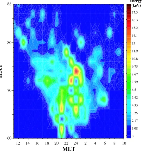
Figure 5 shows that the peak energy grows towards the Magnetic Local Time (MLT) midnight, where also the most intense aurora occur. The highest peak energies appear at and around 20:00–24:00 MLT and at and around 70 ILAT. The morning sector in particular is dominated by low acceleration energies. Events at 80◦ILAT or higher typically have low peak energies as well as low energy flux values (<1 mW/m2). In general, the highest energies appear at the times and places where most of the inverted-V observations are found: around 21:00 MLT and 70–75◦ILAT.
The Magnetic Local Time (MLT) distribution of the inverted-V’s in Fig. 6 shows that most of them take place in the evening and pre-midnight sector around 21:00– 23:00 MLT. This behaviour agrees with that of the overall auroral activity. The MLT distribution in Fig. 6 is normalised by the time FAST spent in each MLT hour bin during the five years. The overlaid curve is the occurrence of about 17 000
[image:4.595.51.282.61.363.2] [image:4.595.312.544.64.359.2]N. Partamies et al.: Statistical study of inverted-V’sPartamies et al.: Statistical Study of inverted-V’s 14435 60 70 80 88 MLT ILAT 0 1.08 2.17 3.25 4.33 5.42 6.5 7.59 8.67 9.75 10.8 11.9 13 14.1 15.2 16.3 17.3 Energy (keV) 8 6 4 2 22 20 18
16 24 10
14 12
Fig. 5. The distribution of the peak energy (colour-coding) as a
function of ILAT and Magnetic Local Time (MLT). Typical invari-ant latitudes for inverted-V observations are 65–75◦. Highest peak energies are usually observed around the magnetic midnight as well as at lower latitudes.
inverted-V and∆T is the time period, during which the V-structure is visible in the satellite data. The typical maximum widths of the structures vary around 130 km (the distribution not shown), and there is a cut-off around 70–90 km. To be able to identify an inverted-V, it must show up in at least three time steps of the data. In the FAST quicklook data, the aver-age time resolution is 5 s. Consequently, the averaver-age speed of the satellite defines the minimum observable inverted-V length to be about 70 km (the distance between the first and the third consecutive observation point).
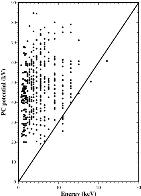
We also determined the cross-polar cap (PC) potential val-ues for each and every inverted-V event. These potential values come from the Super Dual Auroral Radar Network (SuperDARN) radar (Greenwald et al., 1995) measurements, where spherical harmonics have been fitted to the recorded line-of-sight velocities to produce a smooth convection ve-locity map and to give an estimate of the cross-polar cap po-tential (Ruohoniemi and Baker, 1998). The scatter plot in Figure 8 suggests that the PC potential is always at least three times larger than the potential drop accelerating the inverted-V particles. This finding indicates that the PC potential plays a role in determining the acceleration potentials of auroral arcs. As Fig. 8 also demonstrates, there is a clear cutoff in the PC values around 20 kV. The upper end of the PC range is not as clear but shows that very high potential values are rarely observed together with the inverted-V type accelera-tion. There is no reliability check performed for the PC po-tential values in this figure. In other words, no events were
12 13 14 15 16 17 18 19 20 21 22 23 24 0 1 2 3 4 5 6 7 8 9 10
0 1.0 MLT Occurrence t All (588) Best (97) 0.5 11
Fig. 6. The distribution of the occurrence of the inverted-V’s in
MLT shows the maximum occurrence in the pre-midnight sector (21–23 MLT) where also other auroral phenomena are most often seen. The red curve presents the occurrence of auroral arcs in MLT according to Syrj¨asuo and Donovan (2004).
rejected because of, for example, a small amount of actual data points in the convection map. It is not a straightforward task to define when the PC potential estimate is good and thus, we rather rely on the fact that a large number of events averages out the uncertainties.
4 Peak energy, arc widths and Kp
To examine in more detail the relation between the inverted-V peak energy, width (fitted FWHM) and Kp index values we divide the data set into sub-groups with peak energies of less than 3 keV (170 events), 3–6 keV (183 events) and over 6 keV (146 events). For these different subsets we plot the distributions of inverted-V widths (Fig. 9) and Kp (Fig. 10). According to Figure 9 most events with the widths less than 60 km have peak energies less than 6 keV (blue and green bars), while most events with the widths larger than 60 km are caused by accelerated electrons with the energies greater than 3 keV (green and red bars). So there is slight tendency for smaller structures to be less accelerated. However, no clear division point or clear relation between energies and
Fig. 5. The distribution of the peak energy (colour-coding) as a
function of ILAT and Magnetic Local Time (MLT). Typical invari-ant latitudes for inverted-V observations are 65–75◦. Highest peak energies are usually observed around the magnetic midnight as well as at lower latitudes.
auroral arcs as a function of MLT (Syrj¨asuo and Donovan, 2004). The arc occurrence curve, too, has been normalised by the total amount of ASC images taken in each MLT sector. The striking similarity of these two distributions supports the idea that the inverted-V’s are the type of acceleration of the auroral arcs.
Kp index is a three-hour index of geomagnetic activity. It is generated based on measurements at 12 or 13 stations around the world, and its values range from 0 to 9. As seen from Fig. 7, the smallKpvalues from one to four are the ones most commonly related to inverted-V’s. This distribution is normalised by an equally numbered random set ofKp val-ues showing that the most typical of allKpvalues is one. In addition to the smooth distribution around the small values, there are about ten inverted-V events taking place during very active conditions,Kp≥8. Provided that the inverted-V’s oc-cur together with well-defined auroral arcs, it sounds natural that the typical magnetic activity related to these processes is low or moderate. During highKpvalues arcs turn into more dynamic aurora, which indicates changes in the particle ac-celeration structures as well. Higher activity may cause fine structures that are beyond the FAST quicklook data resolu-tion. It may also result in more asymmetric events that, in this study, are not classified as inverted-V’s.
The maximum width of an inverted-V, as we call it, is the total length of the structure as seen by the satellite. This is
Partamies et al.: Statistical Study of inverted-V’s
5
60 70 80 88 MLT ILAT 0 1.08 2.17 3.25 4.33 5.42 6.5 7.59 8.67 9.75 10.8 11.9 13 14.1 15.2 16.3 17.3 Energy (keV) 8 6 4 2 22 20 18
16 24 10
14 12
Fig. 5. The distribution of the peak energy (colour-coding) as a
function of ILAT and Magnetic Local Time (MLT). Typical invari-ant latitudes for inverted-V observations are 65–75◦. Highest peak
energies are usually observed around the magnetic midnight as well as at lower latitudes.
inverted-V and
∆
T
is the time period, during which the
V-structure is visible in the satellite data. The typical maximum
widths of the structures vary around 130 km (the distribution
not shown), and there is a cut-off around 70–90 km. To be
able to identify an inverted-V, it must show up in at least three
time steps of the data. In the FAST quicklook data, the
aver-age time resolution is 5 s. Consequently, the averaver-age speed
of the satellite defines the minimum observable inverted-V
length to be about 70 km (the distance between the first and
the third consecutive observation point).
We also determined the cross-polar cap (PC) potential
val-ues for each and every inverted-V event. These potential
values come from the Super Dual Auroral Radar Network
(SuperDARN) radar (Greenwald et al., 1995) measurements,
where spherical harmonics have been fitted to the recorded
line-of-sight velocities to produce a smooth convection
ve-locity map and to give an estimate of the cross-polar cap
po-tential (Ruohoniemi and Baker, 1998). The scatter plot in
Figure 8 suggests that the PC potential is always at least three
times larger than the potential drop accelerating the
inverted-V particles. This finding indicates that the PC potential plays
a role in determining the acceleration potentials of auroral
arcs. As Fig. 8 also demonstrates, there is a clear cutoff in
the PC values around 20 kV. The upper end of the PC range
is not as clear but shows that very high potential values are
rarely observed together with the inverted-V type
accelera-tion. There is no reliability check performed for the PC
po-tential values in this figure. In other words, no events were
12 13 14 15 16 17 18 19 20 21 22 23 24 0 1 2 3 4 5 6 7 8 9 10 0 1.0 MLT Occurrence t All (588) Best (97) 0.5 11
Fig. 6. The distribution of the occurrence of the inverted-V’s in
MLT shows the maximum occurrence in the pre-midnight sector (21–23 MLT) where also other auroral phenomena are most often seen. The red curve presents the occurrence of auroral arcs in MLT according to Syrj¨asuo and Donovan (2004).
rejected because of, for example, a small amount of actual
data points in the convection map. It is not a straightforward
task to define when the PC potential estimate is good and
thus, we rather rely on the fact that a large number of events
averages out the uncertainties.
4
Peak energy, arc widths and Kp
To examine in more detail the relation between the
inverted-V peak energy, width (fitted FWHM) and Kp index values
we divide the data set into sub-groups with peak energies of
less than 3 keV (170 events), 3–6 keV (183 events) and over
6 keV (146 events). For these different subsets we plot the
distributions of inverted-V widths (Fig. 9) and Kp (Fig. 10).
According to Figure 9 most events with the widths less than
60 km have peak energies less than 6 keV (blue and green
bars), while most events with the widths larger than 60 km
are caused by accelerated electrons with the energies greater
than 3 keV (green and red bars). So there is slight tendency
for smaller structures to be less accelerated. However, no
clear division point or clear relation between energies and
Fig. 6. The distribution of the occurrence of the inverted-V’s in
MLT shows the maximum occurrence in the pre-midnight sector (21:00–23:00 MLT) where also other auroral phenomena are most often seen. The red curve presents the occurrence of auroral arcs in MLT according to Syrj¨asuo and Donovan (2004).
S=VSAT·1T, whereSis the maximum length,VSAT∼=7 km/s is the average speed of the satellite as it passes an inverted-V and1T is the time period, during which the V-structure is visible in the satellite data. The typical maximum widths of the structures vary around 130 km (the distribution not shown), and there is a cut-off around 70–90 km. To be able to identify an inverted-V, it must show up in at least three time steps of the data. In the FAST quicklook data, the av-erage time resolution is 5 s. Consequently, the avav-erage speed of the satellite defines the minimum observable inverted-V length to be about 70 km (the distance between the first and the third consecutive observation point).
We also determined the cross-polar cap (PC) potential val-ues for each and every inverted-V event. These potential values come from the Super Dual Auroral Radar Network (SuperDARN) radar (Greenwald et al., 1995) measurements, where spherical harmonics have been fitted to the recorded line-of-sight velocities to produce a smooth convection ve-locity map and to give an estimate of the cross-polar cap potential (Ruohoniemi and Baker, 1998). The scatter plot in Fig. 8 suggests that the PC potential is always at least three times larger than the potential drop accelerating the
[image:5.595.310.542.64.361.2] [image:5.595.55.283.67.311.2]1444
6
N. Partamies et al.: Statistical study of inverted-V’sPartamies et al.: Statistical Study of inverted-V’s
0 1 2 3 4 5 6 7 8
0 100 190
Kp index
Normalised number of events
All (588) Best (97)
Fig. 7. Distribution of Kp index values related to the inverted-V’s.
The inverted-V’s are typically recorded during quiet times or mod-erate magnetic activity (Kp 1–4). The distribution is divided by the occurrence frequency of each Kp value in a randomly selected data set.
widths can be found. Any structure size can be associated
with any energy range.
The Kp index distributions of the same peak energy
sub-sets are plotted in Figure 10. Similarly to the width
distri-butions of the previous figure, there is no clear Kp
separa-tion for different energies. But when Kp is less than 2 the
inverted-V’s are often caused by electrons with energies less
than 6 keV, while for Kp higher than 2 the electron energies
are usually higher than 3 keV. So, higher acceleration
ener-gies tend to occur in more active conditions.
5
Gaussian fits
To be able to compare the inverted-V scale sizes to the ones
of the auroral arcs and to better define the V widths, we fitted
the Gaussian function to the energy flux curve of the V
struc-tures. Because the subset of the best events and the whole
data set behaved similarly for all other parameters presented
in this paper, the whole data set was fitted. An example of
an energy flux enhancement corresponding to an inverted-V
is shown in the left panel of Figure 11. This example event
is the same one that was shown in Figure 1. The energy flux
is given as a function of distance (along the FAST trajectory)
at the altitude of 100 km.
Prior to the fit, the offsets of the energy flux curves were
manually removed and thus, our fitting routine contains only
0 10 20 30
0 10 20 30 40 50 60 70 80 90
Energy (keV)
[image:6.595.51.280.61.362.2] [image:6.595.311.544.65.388.2]PC potential (kV)
Fig. 8. Cross-polar cap potential measured at the times of the inverted-V observations show that the polar cap potential (Y-axis) is always at least three times larger (solid line) than the peak energy of the inverted-V (X-axis).
three free parameters: the amplitude of the Gaussian curve
A
1, position of its maximum
A
2and the full-width
half-maximum (FWHM) value
A
3. The offset was set to be the
minimum (background) value of the curve prior to the
en-hancement in order to keep as many data points as possible,
since in many cases there were only a few points in total.
The mathematical form of the Gaussian function can now be
written as
y
=
A
1exp
(
−
(
x
−
A
2)
2/
2
A
23)
.
For each event, the residual normalised by the energy flux
amplitude was defined as
R
=
pP
((y
−
m)
2)
/A
1
, where
y
is the Gaussian curve value and
m
is the corresponding
measured energy flux value. We rejected the fits whenever
R
≥
20
% and accepted all fits with
R
≤
10
%. This left
us with 269 acceptably fitted events. An example of a good
fit is shown on the right hand side in Figure 11, and the
dis-tribution of the FWHM values of the fitted inverted-V’s can
be seen in Figure 12. The widths in these plots have been
determined by using the spacecraft average velocity during
each inverted-V event. The typical width of these structures
is 20–40 km and the shape of the distribution slope is
ap-proximately exponential. There is again a cutoff on smaller
widths that is due to the temporal resolution of the
quick-look data and consequently, the minimum observable size.
The minimum observable size for the maximum width of the
inverted-V’s was defined to be about 70 km. Since FWHM
values are the e-fold values of the energy flux curves the
min-imum observable size is clearly smaller in this examination
Fig. 7. Distribution ofKpindex values related to the inverted-V’s.
The inverted-V’s are typically recorded during quiet times or mod-erate magnetic activity (Kp1–4). The distribution is divided by the
occurrence frequency of eachKpvalue in a randomly selected data
set.
inverted-V particles. This finding indicates that the PC po-tential plays a role in determining the acceleration popo-tentials of auroral arcs. As Fig. 8 also demonstrates, there is a clear cutoff in the PC values around 20 kV. The upper end of the PC range is not as clear but shows that very high potential values are rarely observed together with the inverted-V type acceleration. There is no reliability check performed for the PC potential values in this figure. In other words, no events were rejected because of, for example, a small amount of ac-tual data points in the convection map. It is not a straightfor-ward task to define when the PC potential estimate is good and thus, we rather rely on the fact that a large number of events averages out the uncertainties.
4 Peak energy, arc widths andKp
To examine in more detail the relation between the inverted-V peak energy, width (fitted FWHM) andKp index values we divide the data set into sub-groups with peak energies of less than 3 keV (170 events), 3–6 keV (183 events) and over 6 keV (146 events). For these different subsets we plot the distributions of inverted-V widths (Fig. 9) andKp(Fig. 10).
6
Partamies et al.: Statistical Study of inverted-V’s
0 1 2 3 4 5 6 7 8
0 100 190
Kp index
Normalised number of events
All (588)
Best (97)
Fig. 7. Distribution of Kp index values related to the inverted-V’s.
The inverted-V’s are typically recorded during quiet times or
mod-erate magnetic activity (Kp 1–4). The distribution is divided by the
occurrence frequency of each Kp value in a randomly selected data
set.
widths can be found. Any structure size can be associated
with any energy range.
The Kp index distributions of the same peak energy
sub-sets are plotted in Figure 10. Similarly to the width
distri-butions of the previous figure, there is no clear Kp
separa-tion for different energies. But when Kp is less than 2 the
inverted-V’s are often caused by electrons with energies less
than 6 keV, while for Kp higher than 2 the electron energies
are usually higher than 3 keV. So, higher acceleration
ener-gies tend to occur in more active conditions.
5
Gaussian fits
To be able to compare the inverted-V scale sizes to the ones
of the auroral arcs and to better define the V widths, we fitted
the Gaussian function to the energy flux curve of the V
struc-tures. Because the subset of the best events and the whole
data set behaved similarly for all other parameters presented
in this paper, the whole data set was fitted. An example of
an energy flux enhancement corresponding to an inverted-V
is shown in the left panel of Figure 11. This example event
is the same one that was shown in Figure 1. The energy flux
is given as a function of distance (along the FAST trajectory)
at the altitude of 100 km.
Prior to the fit, the offsets of the energy flux curves were
manually removed and thus, our fitting routine contains only
0 10 20 30
0 10 20 30 40 50 60 70 80 90
Energy (keV)
PC potential (kV)
Fig. 8.
Cross-polar cap potential measured at the times of the
inverted-V observations show that the polar cap potential (Y-axis)
is always at least three times larger (solid line) than the peak energy
of the inverted-V (X-axis).
three free parameters: the amplitude of the Gaussian curve
A
1, position of its maximum
A
2and the full-width
half-maximum (FWHM) value
A
3. The offset was set to be the
minimum (background) value of the curve prior to the
en-hancement in order to keep as many data points as possible,
since in many cases there were only a few points in total.
The mathematical form of the Gaussian function can now be
written as
y
=
A
1exp
(
−
(
x
−
A
2)
2/
2
A
23)
.
For each event, the residual normalised by the energy flux
amplitude was defined as
R
=
pP
((y
−
m)
2)
/A
1
, where
y
is the Gaussian curve value and
m
is the corresponding
measured energy flux value. We rejected the fits whenever
R
≥
20
% and accepted all fits with
R
≤
10
%. This left
us with 269 acceptably fitted events. An example of a good
fit is shown on the right hand side in Figure 11, and the
dis-tribution of the FWHM values of the fitted inverted-V’s can
be seen in Figure 12. The widths in these plots have been
determined by using the spacecraft average velocity during
each inverted-V event. The typical width of these structures
is 20–40 km and the shape of the distribution slope is
ap-proximately exponential. There is again a cutoff on smaller
widths that is due to the temporal resolution of the
quick-look data and consequently, the minimum observable size.
The minimum observable size for the maximum width of the
inverted-V’s was defined to be about 70 km. Since FWHM
values are the e-fold values of the energy flux curves the
min-imum observable size is clearly smaller in this examination
Fig. 8. Cross-polar cap potential measured at the times of the
inverted-V observations show that the polar cap potential (Y-axis) is always at least three times larger (solid line) than the peak energy of the inverted-V (X-axis).
According to Fig. 9 most events with the widths less than 60 km have peak energies less than 6 keV (blue and green bars), while most events with the widths larger than 60 km are caused by accelerated electrons with the energies greater than 3 keV (green and red bars). So there is slight tendency for smaller structures to be less accelerated. However, no clear division point or clear relation between energies and widths can be found. Any structure size can be associated with any energy range.
TheKp index distributions of the same peak energy sub-sets are plotted in Fig. 10. Similarly to the width distributions of the previous figure, there is no clearKpseparation for dif-ferent energies. But whenKpis less than 2 the inverted-V’s are often caused by electrons with energies less than 6 keV, while forKphigher than 2 the electron energies are usually higher than 3 keV. So, higher acceleration energies tend to occur in more active conditions.
N. Partamies et al.: Statistical study of inverted-V’s
Partamies et al.: Statistical Study of inverted-V’s
14457
0 10 20 30 40 50 60 70 80 90 100 110 120 130 140 150 160 0
10 20 30
FWHM (km)
Number of envents
Eav < 3keV
3keV < Eav < 6keV
[image:7.595.309.543.62.391.2]Eav > 6keV
Fig. 9. Distribution of full-width half-maximum (FWHM) values
of the inverted-V’s for events with peak energies of less than 3 keV
(blue), between 3 and 6 keV (green), and more than 6 keV (red).
but cannot be exactly determined because it depends on the
energy flux maximum of each event.
The reference data set in Figure 12 is the distribution of the
widths of the optical auroral arcs as observed by the
CANO-PUS all-sky camera in Gillam (Knudsen et al., 2001). The
fitting of the arc brightness profiles by Knudsen et al. (2001)
was performed in a similar manner, and also this optical arc
distribution slopes in an exponential way, but the peak
ap-pears at somewhat smaller values (10 km). The inverted-V
widths might shift to the smaller values, too, if the
high-resolution particle data was used in the event selection. The
similar behaviour of these two data sets suggest that the
meso-scale auroral arcs are the visual traces of the
inverted-V’s seen in the FAST low resolution data. Energy flux is
generally a good proxy for auroral brightness, but here the
different spatial resolutions of the ground-based imager and
the polar orbiting satellite result in slightly different
typi-cally observed scale sizes. To be able to tell whether these
inverted-V’s exactly correspond to single same size arcs or
a system of narrower multiple arcs would require conjugate
measurements from the ground.
6
Discussion
Many things that this statistical study brought up are
simi-lar to the occurrence of other auroral phenomena.
Observa-tions of upgoing ion beams (Collin et al., 1998; Janhunen
0 1 2 3 4 5 6 7 8
0 10 20 30 40 50 60
Kp index
Number of events
Eav < 3keV
3keV < Eav < 6keV
Eav > 6keV
Fig. 10. Distribution of Kp index during the inverted-V’s for events
with peak energies of less than 3 keV (blue), between 3 and 6 keV
(green), and more than 6 keV (red).
8.49 8.5 8.51 0.08
10
UT (hours)
Energy flux (mW/m
2
)
−80 0 100 200
0 10
Distance (km)
Energy flux (mW/m2)
Fig. 11. An example of an energy flux peak within an inverted-V
(left hand side) as well as the fitted Gaussian curve to the energy
flux (right hand side). The diamonds represent the data points and
the vertical lines mark the start and end times of the event
corre-sponding to the first and last pink spots in Figure 1.
[image:7.595.52.283.64.403.2]et al., 2004) showed a peak occurrence in ILAT 68
◦–71
◦,
Fig. 9. Distribution of full-width half-maximum (FWHM) values
of the inverted-V’s for events with peak energies of less than 3 keV (blue), between 3 and 6 keV (green), and more than 6 keV (red).
5 Gaussian fits
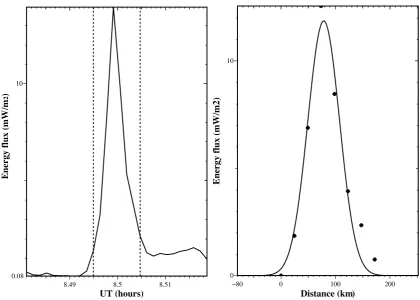
To be able to compare the inverted-V scale sizes to the ones of the auroral arcs and to better define the V widths, we fitted the Gaussian function to the energy flux curve of the V struc-tures. Because the subset of the best events and the whole data set behaved similarly for all other parameters presented in this paper, the whole data set was fitted. An example of an energy flux enhancement corresponding to an inverted-V is shown in the left panel of Fig. 11. This example event is the same one that was shown in Fig. 1. The energy flux is given as a function of distance (along the FAST trajectory) at the altitude of 100 km.
Prior to the fit, the offsets of the energy flux curves were manually removed and thus, our fitting routine contains only three free parameters: the amplitude of the Gaussian curve
A1, position of its maximum A2 and the full-width half-maximum (FWHM) valueA3. The offset was set to be the minimum (background) value of the curve prior to the en-hancement in order to keep as many data points as possible, since in many cases there were only a few points in total.
Partamies et al.: Statistical Study of inverted-V’s 7
0 10 20 30 40 50 60 70 80 90 100 110 120 130 140 150 160 0
10 20 30
FWHM (km)
Number of envents
Eav < 3keV
3keV < Eav < 6keV
Eav > 6keV
Fig. 9. Distribution of full-width half-maximum (FWHM) values
of the inverted-V’s for events with peak energies of less than 3 keV (blue), between 3 and 6 keV (green), and more than 6 keV (red).
but cannot be exactly determined because it depends on the energy flux maximum of each event.
The reference data set in Figure 12 is the distribution of the widths of the optical auroral arcs as observed by the CANO-PUS all-sky camera in Gillam (Knudsen et al., 2001). The fitting of the arc brightness profiles by Knudsen et al. (2001) was performed in a similar manner, and also this optical arc distribution slopes in an exponential way, but the peak ap-pears at somewhat smaller values (10 km). The inverted-V widths might shift to the smaller values, too, if the high-resolution particle data was used in the event selection. The similar behaviour of these two data sets suggest that the meso-scale auroral arcs are the visual traces of the inverted-V’s seen in the FAST low resolution data. Energy flux is generally a good proxy for auroral brightness, but here the different spatial resolutions of the ground-based imager and the polar orbiting satellite result in slightly different typi-cally observed scale sizes. To be able to tell whether these inverted-V’s exactly correspond to single same size arcs or a system of narrower multiple arcs would require conjugate measurements from the ground.
6 Discussion
Many things that this statistical study brought up are simi-lar to the occurrence of other auroral phenomena. Observa-tions of upgoing ion beams (Collin et al., 1998; Janhunen
0 1 2 3 4 5 6 7 8
0 10 20 30 40 50 60
Kp index
Number of events
Eav < 3keV
3keV < Eav < 6keV
Eav > 6keV
Fig. 10. Distribution of Kp index during the inverted-V’s for events
with peak energies of less than 3 keV (blue), between 3 and 6 keV (green), and more than 6 keV (red).
8.49 8.5 8.51 0.08
10
UT (hours)
Energy flux (mW/m
2
)
−80 0 100 200 0
10
Distance (km)
Energy flux (mW/m2)
Fig. 11. An example of an energy flux peak within an inverted-V
(left hand side) as well as the fitted Gaussian curve to the energy flux (right hand side). The diamonds represent the data points and the vertical lines mark the start and end times of the event corre-sponding to the first and last pink spots in Figure 1.
et al., 2004) showed a peak occurrence in ILAT 68◦–71◦,
Fig. 10. Distribution ofKpindex during the inverted-V’s for events
with peak energies of less than 3 keV (blue), between 3 and 6 keV (green), and more than 6 keV (red).
The mathematical form of the Gaussian function can now be written asy=A1exp(−(x−A2)2/2A23).
For each event, the residual normalised by the energy flux amplitude was defined asR=pP((y−m)2)/A
1, where
y is the Gaussian curve value and mis the corresponding measured energy flux value. We rejected the fits whenever
R≥20% and accepted all fits withR≤10%. This left us with 269 acceptably fitted events. An example of a good fit is shown on the right hand side in Fig. 11, and the distribution of the FWHM values of the fitted inverted-V’s can be seen in Fig. 12. The widths in these plots have been determined by using the spacecraft average velocity during each inverted-V event. The typical width of these structures is 20–40 km and the shape of the distribution slope is approximately ex-ponential. There is again a cutoff on smaller widths that is due to the temporal resolution of the quicklook data and con-sequently, the minimum observable size. The minimum ob-servable size for the maximum width of the inverted-V’s was defined to be about 70 km. Since FWHM values are the e-fold values of the energy flux curves the minimum observ-able size is clearly smaller in this examination but cannot
1446 N. Partamies et al.: Statistical study of inverted-V’s
Partamies et al.: Statistical Study of inverted-V’s
7
0 10 20 30 40 50 60 70 80 90 100 110 120 130 140 150 160
0
10
20
30
FWHM (km)
Number of envents
Eav < 3keV
3keV < Eav < 6keV
Eav > 6keV
Fig. 9. Distribution of full-width half-maximum (FWHM) values
of the inverted-V’s for events with peak energies of less than 3 keV
(blue), between 3 and 6 keV (green), and more than 6 keV (red).
but cannot be exactly determined because it depends on the
energy flux maximum of each event.
The reference data set in Figure 12 is the distribution of the
widths of the optical auroral arcs as observed by the
CANO-PUS all-sky camera in Gillam (Knudsen et al., 2001). The
fitting of the arc brightness profiles by Knudsen et al. (2001)
was performed in a similar manner, and also this optical arc
distribution slopes in an exponential way, but the peak
ap-pears at somewhat smaller values (10 km). The inverted-V
widths might shift to the smaller values, too, if the
high-resolution particle data was used in the event selection. The
similar behaviour of these two data sets suggest that the
meso-scale auroral arcs are the visual traces of the
inverted-V’s seen in the FAST low resolution data. Energy flux is
generally a good proxy for auroral brightness, but here the
different spatial resolutions of the ground-based imager and
the polar orbiting satellite result in slightly different
typi-cally observed scale sizes. To be able to tell whether these
inverted-V’s exactly correspond to single same size arcs or
a system of narrower multiple arcs would require conjugate
measurements from the ground.
6
Discussion
Many things that this statistical study brought up are
simi-lar to the occurrence of other auroral phenomena.
Observa-tions of upgoing ion beams (Collin et al., 1998; Janhunen
0
1
2
3
4
5
6
7
8
0
10
20
30
40
50
60
Kp index
Number of events
Eav < 3keV
3keV < Eav < 6keV
Eav > 6keV
Fig. 10. Distribution of Kp index during the inverted-V’s for events
with peak energies of less than 3 keV (blue), between 3 and 6 keV
(green), and more than 6 keV (red).
8.49 8.5 8.51 0.08
10
UT (hours)
Energy flux (mW/m
2
)
−80 0 100 200
0 10
Distance (km)
[image:8.595.87.508.63.363.2]Energy flux (mW/m2)
Fig. 11. An example of an energy flux peak within an inverted-V
(left hand side) as well as the fitted Gaussian curve to the energy
flux (right hand side). The diamonds represent the data points and
the vertical lines mark the start and end times of the event
corre-sponding to the first and last pink spots in Figure 1.
et al., 2004) showed a peak occurrence in ILAT 68
◦
–71
◦
,
Fig. 11. An example of an energy flux peak within an inverted-V (left hand side) as well as the fitted Gaussian curve to the energy flux (right
hand side). The diamonds represent the data points and the vertical lines mark the start and end times of the event corresponding to the first and last pink spots in Fig. 1.
be exactly determined because it depends on the energy flux maximum of each event.
The reference data set in Fig. 12 is the distribution of the widths of the optical auroral arcs as observed by the CANO-PUS all-sky camera in Gillam (Knudsen et al., 2001). The fitting of the arc brightness profiles by Knudsen et al. (2001) was performed in a similar manner, and also this optical arc distribution slopes in an exponential way, but the peak ap-pears at somewhat smaller values (10 km). The inverted-V widths might shift to the smaller values, too, if the high-resolution particle data was used in the event selection. The similar behaviour of these two data sets suggest that the meso-scale auroral arcs are the visual traces of the inverted-V’s seen in the FAST low resolution data. Energy flux is generally a good proxy for auroral brightness, but here the different spatial resolutions of the ground-based imager and the polar orbiting satellite result in slightly different typi-cally observed scale sizes. To be able to tell whether these inverted-V’s exactly correspond to single same size arcs or a system of narrower multiple arcs would require conjugate measurements from the ground.
6 Discussion
Many things that this statistical study brought up are similar to the occurrence of other auroral phenomena. Observations of upgoing ion beams (Collin et al., 1998; Janhunen et al., 2004) showed a peak occurrence in ILAT 68◦–71◦, which are
the average auroral oval latitudes as well as the typical lati-tudes of the inverted-V observations of this study. The mag-netic local time and the invariant latitude distribution of the inverted-V’s are similar to those of the probability of accel-erated electrons (Newell et al., 1996) and the average auroral intensity (Liou et al., 1997). One significant difference, how-ever, is that V-structures are also observed at the invariant latitudes of 80◦, where the probability of electron accelera-tion and the average auroral intensity are negligible.
Seasonal variation of other auroral phenomena, such as average auroral luminosity in ultraviolet (Liou et al., 1997), occurrence frequency of upward flowing ion beams (Collin et al., 1998; Janhunen et al., 2004), cosmic radio noise ab-sorption (Yamagishi et al., 1998), ionospheric narrow-band ELF emissions (Satio et al., 1987), occurrence of auroral electromagnetic ion cyclotron (EMIC) waves (Erlandson and Zanetti, 1998), occurrence of auroral kilometric radiation (AKR) (Kumamoto and Oya, 1998), particle acceleration