A constrained multi-objective surrogate-based optimization algorithm

(1)

A Constrained Multi-Objective Surrogate-Based Optimization

Algorithm

Prashant Singh, Ivo Couckuyt, Francesco Ferranti and Tom Dhaene

Abstract— Surrogate models or metamodels are widely used in the realm of engineering for design optimization to minimize the number of computationally expensive simulations. Most practical problems often have conflicting objectives, which lead to a number of competing solutions which form a Pareto front. Multi-objective surrogate-based constrained optimization algorithms have been proposed in literature, but handling constraints directly is a relatively new research area. Most algorithms proposed to directly deal with multi-objective op-timization have been evolutionary algorithms (Multi-Objective Evolutionary Algorithms - MOEAs). MOEAs can handle large design spaces but require a large number of simulations, which might be infeasible in practice, especially if the constraints are expensive. A multi-objective constrained optimization algorithm is presented in this paper which makes use of Kriging models, in conjunction with multi-objective probability of improvement (PoI) and probability of feasibility (PoF) criteria to drive the sample selection process economically. The efficacy of the pro-posed algorithm is demonstrated on an analytical benchmark function, and the algorithm is then used to solve a microwave filter design optimization problem.

I. INTRODUCTION

E

NGINEERING design optimization of complex systems such as aircraft, electronic filters, wireless sensors, etc. often involves expensive simulations. Wang and Shan [1] cite the example of an automotive crash simulation conducted by Ford Motor Company which takes anywhere between 36 and 160 hours to complete. A two variable optimization problem would take 75 days to 11 months to solve using these estimates, which is unacceptable in practice. This time-to-completion can be drastically scaled down if a cheaper replacement is used instead of the expensive simulator. Specifically, this work is concerned with data-based black-box approximations, also known as surrogate models or

metamodels.

Surrogate models may be used as full replacements of the underlying simulators for all intents and purposes (global

surrogate models), or may cover only a region within the entire design space (localsurrogate models). Local surrogate models are often used in global design optimization frame-works [2]. The methodology of using surrogate models to aid the process of design optimization is called surrogate based optimization (SBO). A SBO problem may be single-objective Prashant Singh, Ivo Couckuyt, Francesco Ferranti and Tom Dhaene are with the Department of Information Technology, iMinds, Ghent University, Ghent 9000, Belgium (email: {prashant.singh, ivo.couckuyt, francesco.ferranti, tom.dhaene}@intec.ugent.be).

This research has been funded by the Interuniversity Attraction Poles Programme BESTCOM initiated by the Belgian Science Policy Office, and the Fund for Scientific Research in Flanders (FWO-Vlaanderen). Ivo Couckuyt and Francesco Ferranti are post-doctoral research fellows of FWO-Vlaanderen.

or multi-objective. This paper proposes a novel SBO algo-rithm for multi-objective optimization problems which may have additional computationally expensive constraints. The optimization solution is given in the form of a set of equally optimal solutions, i.e., the Pareto set.

This paper is organized as follows: Section II describes the use of surrogate models in design optimization. The proposed algorithm is presented in Section III and its efficacy is tested on analytical and real-world problems in Section IV. Finally, the conclusions are drawn in Section V.

II. MULTI-OBJECTIVESURROGATEBASED OPTIMIZATION

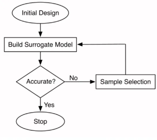
A typical surrogate modeling scenario is shown in Fig. 1. The idea is to evaluate the simulator at a few carefully chosen points in the design space, so as to maximize information gain. In the case of global surrogate modeling, the goal is to mimic the behavior of the simulator as closely as possible, and the sample selection scheme chooses additional samples to achieve this objective with a minimal number of expensive samples.

Initial Design

Build Surrogate Model

Accurate?

Stop

Sample Selection

Yes No

Fig. 1. Surrogate Modeling Flowchart.

In the case of surrogate-based optimization (SBO) the aim is to find the global optimum, and the sample selec-tion scheme selects addiselec-tional samples to guide the search towards the optimum. SBO methods have been widely used in various fields such as aerospace, electromagnetics, metal-lurgy, etc. [3]

The past decade has seen widespread use of SBO methods to solve single-objective optimization problems. However, most problems in the real-world are multi-objective with the objectives often in conflict with each other, and some

(2)

complex problems have additional constraints (over objec-tives, or inputs). These constraints in turn may also be computationally expensive to evaluate and, hence, applying traditional constrained optimization methods may be too time-consuming. Multi-objective optimization methods result in multiple solutions, the Pareto set. Each solution in the Pareto set can not be improved with respect to a particular objective without compromising on another objective.

Most methods in literature to solve multi-objective opti-mization problems directly have been evolutionary in nature. Examples are theNon-dominated Sorting Genetic Algorithm

- II (NSGA-II) [8], the Strength Pareto Evolutionary Algo-rithm 2(SPEA2) [9] and theS-Metric Selection Evolutionary

MultiObjective Algorithm (SMS-EMOA) [10].

Although the resulting Pareto sets are convenient, multi-objective evolutionary algorithms usually require a very large number of simulations, which is a prohibitive factor when simulations are expensive. Couckuyt et al. [4] presented a MOSBO algorithm (Efficient Multiobjective Optimization algorithm) which uses multi-objective formulations of prob-ability of improvement (PoI) and expected improvement (EI) criteria [6] with Kriging models. EMO is more efficient in terms of number of function evaluations as compared to evolutionary methods.

The algorithm proposed in this work uses the hypervolume-based PoI criterion described in [4] to handle multiple objectives and utilizes the Probability of Feasibility (PoF) criterion to handle computationally expensive constraints.

III. EFFICIENTCONSTRAINEDMULTI-OBJECTIVE OPTIMIZATIONALGORITHM(ECMO)

The sampling criteria employed by the proposed ECMO algorithm make use of Kriging models to drive the op-timization process. Kriging models are very popular and widely used in surrogate modeling. A thorough mathematical treatment has been given by Forrester et al. [5]. A basic introduction is presented below. Multi-objective versions of the hypervolume-based probability of improvement (PoI) [4] and the probability of feasibility (PoF) are described in subsequent sections.

A. Kriging

Given a set of𝑛samples𝑋, (x₁, ...,x_n)′in𝑑dimensions mapped to function values (𝑦1, ..., 𝑦𝑛)′,

𝑋= (x1, ...,xn)′ (1)

Kriging is composed of two components. The first com-ponent is a regressor ℎ(𝑥), while the second component is a centred Gaussian process 𝑍, which is constructed with variance 𝜎2 and correlation matrix𝜓through the residuals.

𝑌(x) =ℎ(x) +𝑍(x). (2)

The regressor is coded in the𝑛×𝑝matrix𝐹 having basis functions𝑏_𝑖(x)for 𝑖= 1...𝑝, 𝐹 = ⎛ ⎜ ⎝ 𝑏1(x1) 𝑏2(x1) ⋅ ⋅ ⋅ 𝑏𝑝(x1) .. . . .. ... 𝑏1(xn) 𝑏2(xn) ⋅ ⋅ ⋅ 𝑏𝑝(xn) ⎞ ⎟ ⎠,

and the 𝑛×𝑛correlation matrix𝜓 is given by,

𝜓= ⎛ ⎜ ⎝ 𝜓(x1,x1) ⋅ ⋅ ⋅ 𝜓(x1,xn) .. . . .. ... 𝜓(xn,x1) ⋅ ⋅ ⋅ 𝜓(xn,xn) ⎞ ⎟ ⎠,

where 𝜓(x_i,x_j) is the correlation function. 𝜓(x_i,x_j) is parameterized by a set of hyperparameters 𝜃. Obtaining an accurate model is highly dependent upon the choice of the correlation function. In this work, the Mat´ern correlation function [11] with𝜈= 3₂ is used for the experiments, which is defined as 𝜓(x,x′₎𝑀𝑎𝑡´𝑒𝑟𝑛 𝜈=3 2 = (1 + √ 3𝑙)𝑒𝑥𝑝(−√3𝑙), (3) where 𝑙= ⎷∑𝑑 𝑖=1 𝜃𝑖(𝑥𝑖−𝑥′𝑖)2.

The hyperparameters 𝜃 are identified by Maximum Like-lihood Estimation (MLE) [4].

B. Hypervolume-based PoI

The single-objective probability of improvement sampling criterion [5] has been widely used in practice, and discussed in literature. The idea is to select subsequent samples such that the current best output value 𝑦_𝑚𝑖𝑛 is improved. Let

ˆ

𝑦(x)be the prediction and 𝑠2(x)be the prediction variance of the Kriging model, then the probability of having an improvement is,

𝑃(𝐼(x)) = Φ(𝑦𝑚𝑖𝑛)

where Φ(𝑡) is the normal cumulative distribution function

Φ(𝑡) = 1 2 ( 1 +𝑒𝑟𝑓(_𝑠𝑡−₍_x𝑦ˆ₎(√x) 2 ))

with mean𝑦ˆ(x)and variance

𝑠2₍_x₎_{, and}_𝑒𝑟𝑓₍_⋅₎ _{is the Gauss error function.}

However, in a multi-objective setting there are several ways to measure the improvement over the current Pareto set. Couckuyt et. al. [4] proposed to use the hypervolume-based PoI for its good performance and fast calculation.

The hypervolume-based PoI is defined as,

𝑃ℎ𝑣(𝐼(x)) =ℋ𝑒𝑥𝑐(x)×𝑃(𝐼(x)),

where ℋ_𝑒𝑥𝑐(x)is the exclusive hypervolume measuring the improvement of a new sample x over the Pareto set and

𝑃(𝐼(x)) is the multi-objective probability of improvement given by, 𝑃(𝐼(x)) = ∫ y∈𝐴 𝑚 ∏ 𝑗=1 𝜙𝑗(𝑦𝑗)𝑑𝑦𝑗,

(3)

with 𝐴 being the non-dominated region (Fig. 2) of the ob-jective space and𝑚being the number of objective functions. The function𝜙_𝑗is the probability density function associated with the Kriging model for the 𝑗′𝑡ℎ objective denoted as

𝜙𝑗(𝑦𝑗)≜𝜙𝑗(𝑦𝑗; ˆ𝑦𝑗(x), 𝑠2𝑗(x)). y 1 y2 Non−dominated region Exclusive hypervolume p f3 f4 f5 f6 fv=7 f1 f2

Fig. 2. Illustration of a Pareto set of two objective functions. The dots represent the Pareto points 𝑓𝑖 , for 𝑖 = 1...𝑣. The integration area A of the hypervolume-based PoI corresponds to the (light and dark) shaded region which is decomposed into cells by a binary partitioning procedure. The exclusive hypervolume of a pointprelative to the Pareto set can be computed from existing cells and corresponds to the dark shaded region.

Identifying𝐴and, hence, evaluating the criterion is rather cumbersome. An efficient algorithm is suggested by Couck-uyt et. al. which is used in this paper. For further information, the reader is referred to Couckuyt et al. [4].

C. Probability of Feasibility

The probability of feasibility (PoF) criterion [6] is well suited to handle expensive constraint functions. Intuitively, the PoF criterion can be seen as a measure of the degree to which a sample satisfies the constraints. The higher the prob-ability, the stronger the indication that the sample satisfies the constraints. Given𝑘constraint functions, each modelled by a Kriging model, the probability of the prediction being greater than the constraint limit can be computed in a manner similar to the probability of improvement. Let𝑔ˆ𝑖(x)be the prediction and 𝑠2_𝑖(x) be the variance of the Kriging model for the 𝑖𝑡ℎ constraint where 𝑖= 1, .., 𝑘, then the probability of feasibility can be defined as

𝑃(𝐹𝑖(x)> 𝑔𝑖𝑚𝑖𝑛) = Φ ( 𝐹𝑖−𝑔ˆ𝑖(x) 𝑠𝑖(x) ) ,

where Φ(𝑡) is the standard normal cumulative distribution function Φ(𝑡) = 1₂

(

1 +𝑒𝑟𝑓(_√𝑡

2)

)

, 𝑔𝑖 the constraint func-tion, 𝑔𝑖_𝑚𝑖𝑛 the limiting constraint value, 𝐹_𝑖(x) = 𝐺_𝑖(x)−

𝑔𝑖

𝑚𝑖𝑛 the measure of feasibility and𝐺𝑖(x)a random variable

for the𝑖𝑡ℎconstraint. The combined probability of feasibility of satisfying𝑘 constraints then becomes

𝑃𝑐𝑜𝑚𝑏𝑖𝑛𝑒𝑑(x) = 𝑘 ∏ 𝑖=1

𝑃(𝐹𝑖(x)> 𝑔𝑚𝑖𝑛𝑖 ). (4)

The final multi-objective criterion 𝛾 used in this work is obtained by multiplying the hypervolume-based PoI with the PoF

𝛾(x) =𝑃ℎ𝑣(𝐼(x))×𝑃𝑐𝑜𝑚𝑏𝑖𝑛𝑒𝑑(x).

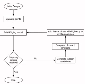
Optimizing this criterion will provide an automatic balance between selecting points which: (i) improve the Pareto set satisfying all the constraints, (ii) improve the accuracy of the Kriging models of the objectives and constraints. The candidates satisfying the constraints will have a high value of 𝑃_{𝑐𝑜𝑚𝑏𝑖𝑛𝑒𝑑}, while the candidates which minimize the ob-jective more will have a high value of𝑃_ℎ𝑣. Thus, candidates having a high 𝛾 value will be more desirable in terms of satisfying the constraints as well as improving the value of the objective function(s). The flowchart of the ECMO algorithm can be seen in Fig. 3.

Initial Design

Evaluate points

Build Kriging model

Stopping criteria reached? Stop Generate random candidates

Compute γ for each

candidate

Add the candidate with highest γ to

existing samples

Yes

No

Fig. 3. Flowchart of the ECMO algorithm.

Since the uncertainty of the Kriging model will be high during the start of the optimization process due to the limited number of samples available, the value of the PoF criterion for candidate samples will not be very close to 0 or 1. As the algorithm iterates and more samples are selected, the uncertainty will decrease and the Kriging model will be more certain and assign probabilities close to 0 or 1 to candidate samples.

Since each objective and each constraint is modeled using a separate Kriging model, the algorithm is prone to slowing down as the number of objectives and constraints (𝑚+𝑘) increases. However, the increase in number of dimensions

𝑑 has a more severe effect on the modeling speed as the complexity of building a Kriging model is cubic in the number of total samples and increases exponentially with the number of dimensions. Typically, the number of samples

(4)

required to build an accurate model is directly proportional to the dimensionality of the problem. As the dimensionality

𝑑of the problem increases, an increasing amount of samples would be needed to train the Kriging model and the speed of model construction will become progressively slower. These limitations can be countered to an extent by using different approximation methods for Kriging [12].

IV. EXAMPLES

The ECMO algorithm is tested on an analytical, and a real-world problem. The analytical example is the Nowacki Beam Problem [13], while the real-world problem is the design of a microwave filter. The experiments are performed using the SUrrogate MOdeling MATLAB1_{Toolbox (SUMO)}

[14], which is freely available for personal non-commercial use. MATLAB’sfminconoptimizer was used to optimize the best candidate selected using the 𝛾 criterion. The stopping criterion used for the experiments was a limit on the number of samples or function evaluations. Other possible stopping criteria include stopping when the model reaches a certain accuracy (e.g. cross-validation error below a specified limit) and a limit on the time (in seconds/minutes/hours) the algorithm takes.

A. Nowacki Beam Problem

Nowacki [13] described a tip-loaded encastre cantilever beam design problem [5] for minimum cross-sectional area and lowest bending stress subject to specified constraints. Considering a rectangular beam of length𝑙= 1.5m, subject to a tip-load 𝐹 = 5 kN, with design variables being height

ℎ and breadth 𝑏 of the beam, the constrained optimization problem can be formulated as:

Min 𝑏,ℎ 𝐴, 𝜎𝐵 for 20 mm< ℎ <250 mm, 10 mm< 𝑏 <50 mm, s.t. 𝛿≤5mm, 𝜎𝐵≤𝜎𝑌, 𝜏≤𝜎𝑌/2, ℎ/𝑏≤10, 𝐹𝐶𝑅𝐼𝑇 ≥𝑓 ×𝐹,

where 𝐴=𝑏×ℎis the cross-sectional area of the beam,

𝜎𝐵 = 6𝐹 𝑙/(𝑏ℎ2) is the bending stress, 𝛿 = 𝐹 𝑙3/(3𝐸𝐼𝑌)

is the maximum tip deflection, 𝜎_𝑌 is the yield stress of the material, 𝜏 = 3𝐹/(2𝑏ℎ) is the maximum allowable shear stress, ℎ/𝑏 is the height-to-breadth ratio, and 𝐹𝐶𝑅𝐼𝑇 = (4/𝑙2₎√_𝐺𝐼_𝑇_𝐸𝐼_𝑍_/₍₁₋_𝜈2₎_{is the failure force of buckling.} Here,𝐼𝑇 = (𝑏3ℎ+𝑏ℎ3)/12,𝐼𝑍 =𝑏3ℎ/12, and𝑓 is a safety factor of two.

1_{MATLAB, The MathWorks Inc., Natick, MA}

The material under consideration is mild steel with yield stress 𝜎_𝑌 = 240 MPa, Young’s modulus 𝐸 = 216.62 GPa,

𝜈 = 0.27and shear modulus 𝐺= 86.65 GPa.

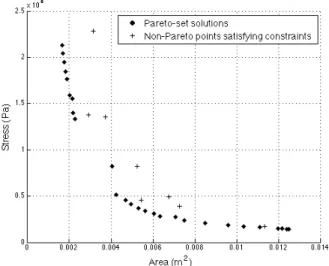
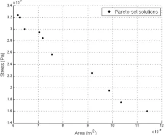
Fig. 4. Non-dominated solutions of the Nowacki beam problem found using ECMO.

Fig. 5. The selected samples for the Nowacki beam problem. The ECMO algorithm was allowed to run for a total of 50 sample points, beginning with a Latin Hypercube of 11 points in addition to the 4 corner points. The result of the proposed algorithm for the Nowacki beam problem can be seen in Fig. 4. The sample points can be seen in Fig. 5. The Pareto front clearly describes the trade-off between the two objectives - at the extreme value of one objective, the other has its least value. It should be noted that there are points which satisfy all the constraints, but are not included in the Pareto set as they are dominated by other solutions.

For the purpose of comparison, the NSGA-II algorithm was used to solve the problem. The population size was set to 10, and the algorithm was allowed to run for 4 generations to match the limit of 50 total function evaluations imposed

(5)

Fig. 6. Non-dominated solutions of the Nowacki beam problem found using NSGA-II.

on ECMO. The resulting Pareto front can be seen in Fig. 6. The ECMO algorithm was able to find 27 non-dominated solutions, as compared to 9 non-dominated solutions found by Forrester et. al. [5] (using multi-objective constrained expected improvement) and 10 found by NSGA-II using the same number of total samples.

Although it can be argued that initializing NSGA-II with a larger population may yield more solutions, that would come at the cost of sacrificing the number of generations.

B. Double Folded Stub Microwave Filter

The ECMO algorithm is used to model a Double Folded Stub (DFS) microwave filter with constraints on its scattering parameters and design parameters. The filter is similar to the one described in Chemmangat et. al. [15].

Fig. 7. Layout of the DFS microwave filter.

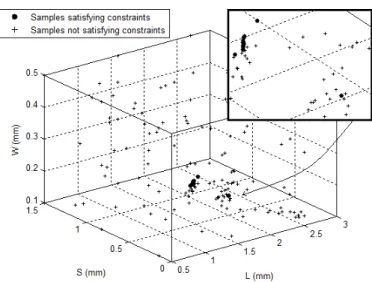
The design variables are the spacing 𝑆 between a folded stub and the main line, the length 𝐿 of each folded stub, and the width 𝑊 of each conductor. The scattering matrix

S(𝑓, 𝑆, 𝐿, 𝑊) is computed using the ADS Momentum EM simulator2_{. The frequency}_𝑓 _{is sampled over the range [5-20]}

GHz using 91 uniformly distributed samples. The substrate is 0.254 mm thick with relative permittivity 𝜖_𝑟equal to 9.9. The scattering matrixS(𝑓, 𝑆, 𝐿, 𝑊)can be written as

2_{Momentum EEsof EDA, Agilent Technologies, Santa Rosa, CA.}

S(𝑓, 𝑆, 𝐿, 𝑊) = [ 𝑆11(𝑓, 𝑆, 𝐿, 𝑊) 𝑆12(𝑓, 𝑆, 𝐿, 𝑊) 𝑆21(𝑓, 𝑆, 𝐿, 𝑊) 𝑆22(𝑓, 𝑆, 𝐿, 𝑊) ] , (5) and is a complex-valued matrix composed of a real and imaginary part.

TABLE I

DESIGN PARAMETERS OF THEDFSMICROWAVE FILTER

Parameter Min Max Spacing 0.15 mm 1.5 mm

Length 0.5 mm 5.0 mm Width 0.1 mm 0.5 mm

The design specifications are formulated in terms of objec-tives and constraints on the scattering parameters and design variables. The constrained optimization problem is defined as Min 𝑆,𝑊,𝐿 −∣𝑆21∣dB, ∣𝑆21∣dB for (5 GHz ≤𝑓 ≤8 GHz, 18 GHz ≤𝑓 ≤20 GHz), (12 GHz ≤𝑓 ≤14 GHz), respectively s.t. 3𝑊 + 2𝑆 ≤2 mm ∣𝑆11∣dB≥-3 dB for 12 GHz≤𝑓 ≤14 GHz ∣𝑆21∣dB ≤-30 dB for 12 GHz≤𝑓 ≤14 GHz ∣𝑆11∣dB≤-10 dB for 5 GHz≤𝑓 ≤8 GHz and 18 GHz≤𝑓 ≤20 GHz ∣𝑆21∣dB≥-3 dB for 5 GHz≤𝑓 ≤8 GHz and 18 GHz≤𝑓 ≤20 GHz where ∣.∣dB= 20𝑙𝑜𝑔10∣.∣and∣.∣indicates the absolute value

operator. It should be noted that the objective −∣𝑆21∣dB

corresponds to the frequency range 𝑓₁ = (5≤𝑓 ≤8,18≤

𝑓 ≤ 20) GHz and objective ∣𝑆21∣dB corresponds to the

frequency range𝑓₂= (12≤𝑓 ≤14)GHz.

The algorithm was allowed to run with a total simulation budget of 150 samples. The initial design was a Latin Hypercube of 50 samples, in addition to 8 corner points. One sample per iteration was added till the sampling budget was exhausted. Each simulation takes approximately a minute on an Intel Core i5 machine with 8 GB RAM. It is desirable to perform as few simulations as possible while searching for possible solutions.

The result of the algorithm can be seen in Fig. 8 and Fig. 9. It can be observed that the hypervolume-based probability of improvement and probability of feasibility sampling criteria drive the sampling towards the region with a high likelihood of having design points which minimize the objectives and satisfy constraints. This leads to a dense clustering which

(6)

Fig. 8. Pareto set for the DFS microwave filter.

Fig. 9. Selected sampling locations for the DFS microwave filter. The region containing the Pareto-optimal solutions is very small and the solutions can be seen in a magnified view.

can be seen in Fig. 9. Since the algorithm is able to zoom in on the interesting region quickly, the approach minimizes the number of expensive simulations required by concentrating on the regions having a high likelihood of containing possible solutions.

The layouts and frequency responses (∣𝑆11∣dB,∣𝑆21∣dB) of

three of the filter designs from the Pareto set are depicted in Figs. 10 - 18. Although each of the solutions in the Pareto set are non-dominated, the designer may prefer one over the other based on different criteria like selecting the solution with the values of the design parameters𝑆,𝐿, or𝑊 which are most suitable for the robustness of the design considering fabrication tolerances.

The stopping criteria also depend on the designer. A de-signer might want to obtain Pareto-optimal solutions rapidly in case there is a need to get the product in the market quickly, or when the designer wants to check possible

so-Fig. 10. Layout of one of the Pareto-optimal DFS filter designs with design variables (𝑆, 𝐿, 𝑊) = (0.7168, 1.7449, 0.1887) mm.

Fig. 11. ∣𝑆₁₁∣response of one of the Pareto-optimal DFS filter designs with design variables (𝑆, 𝐿, 𝑊) = (0.7168, 1.7449, 0.1887) mm.

Fig. 12. ∣𝑆21∣response of one of the Pareto-optimal DFS filter designs with design variables (𝑆, 𝐿, 𝑊) = (0.7168, 1.7449, 0.1887) mm.

(7)

Fig. 13. Layout of one of the Pareto-optimal DFS filter designs with design variables (𝑆, 𝐿, 𝑊) = (0.7236, 1.7536, 0.1824) mm.

Fig. 16. Layout of one of the Pareto-optimal DFS filter designs with design variables (𝑆, 𝐿, 𝑊) = (0.7292, 1.7159, 0.1805) mm.

(8)

lutions for different values of constraints/objectives. In such cases the sampling budget will be small. On the other hand, a designer might also want the freedom to obtain a large number of competing Pareto-optimal solutions so that they can later be evaluated based on other parameters.

V. CONCLUSIONS

We have presented the ECMO algorithm to solve compu-tationally expensive constrained multi-objective optimization problems which uses Kriging models in conjunction with probability of improvement (PoI) and probability of feasi-bility (PoF). The ECMO algorithm performed as expected on test problems and has the ability to solve multi-objective constrained optimization problems. The algorithm however suffers from the well-known limitations of surrogate mod-eling methods with respect to the limited input dimension-ality of the problems which can be handled. However, the ECMO algorithm can be applied to problems having up to 7 objectives, which is sufficient for most real-world problems. Future work will compare the ECMO algorithm with existing methods to solve constrained multi-objective optimization problems.

REFERENCES

[1] G. Wang and S. Shan, “Review of metamodeling techniques in support of engineering design optimization,”Journal of Mechanical Design, vol. 129, pp. 370, 2007.

[2] N. M. Alexandrov, J. E. Dennis Jr, R. M. Lewis, and V. Torczon, “A trust-region framework for managing the use of approximation models in optimization,”Structural Optimization, vol. 15, no. 1, pp. 16-23, 1998.

[3] S. Koziel and L. Leifsson (eds.), “Surrogate-Based Modeling and Optimization,”Applications in Engineering, ISBN 978-1-4614-7551-4, Springer, 2013.

[4] I. Couckuyt, D. Deschrijver and T. Dhaene, “Fast Calculation of the Multiobjective Probability of Improvement and Expected Improvement Criteria for Pareto Optimization,”Journal of Global Optimization, In Print, 2013.

[5] A. Forrester, A. Sobester, A. Keane, “Engineering Design via Surro-gate Modelling: A Practical Guide,” ISBN 978-0-470-06068-1, Wiley, 2008.

[6] A. Forrester and A. Keane, “Recent advances in surrogate-based optimization,”Progress in Aerospace Sciences, vol. 45, no. 1, pp. 50-79, 2009.

[7] J. Martin and T. Simpson, “Use of kriging models to approximate deterministic computer models,”AIAA journal, vol. 43, no 4, pp. 853-863, 2005.

[8] K. Deb, A. Pratap, S. Agarwal, T. Meyarivan, “A fast and elitist multiobjective genetic algorithm: NSGA-II,” IEEE Transactions on

Evolutionary Computation, vol. 6, no. 2, pp. 182-197, 2002.

[9] E. Zitzler, M. Laumanns, and L. Thiele, “SPEA2: Improving the Strength Pareto Evolutionary Algorithm,” Technical Report, Swiss

Federal Institute of Technology, 2001.

[10] N. Beume, B. Naujoks, M. Emmerich, “SMS-EMOA: Multiobjective selection based on dominated hypervolume,” European Journal of

Operational Research, vol. 181, no. 3, pp. 1653-1669, 2007.

[11] M. Stein, “Interpolation of spatial data: some theory for kriging,” ISBN 978-0-387-98629-6, Springer, 1999.

[12] K. Chalupka, C. K. Williams, and I. Murray, “A framework for evaluating approximation methods for Gaussian process regression,”

The Journal of Machine Learning Research, vol. 14 no. 1, pp.

333-350, 2013.

[13] H. Nowacki, (1980) “Modelling of design decisions for CAD,”CAD

Modelling, Systems Engineering, CAD-Systems, Lecture Notes in

Computer Science, Springer-Verlag, Berlin, 1980.

[14] D. Gorissen, I. Couckuyt, P. Demeester, T. Dhaene, K. Crombecq, “A Surrogate Modeling and Adaptive Sampling Toolbox for Computer Based Design,”Journal of Machine Learning Research, vol. 11, pp. 2051-2055, July 2010.

[15] K. Chemmangat, F. Ferranti, T. Dhaene, L. Knockaert, “Gradient-based optimization using parametric sensitivity macromodels,”International Journal of Numerical Modelling: Electronic Networks, Devices and