Modeling of Sales Forecasting in Retail Using Soft
Computing Techniques
Lu´ıs Lobo da Costa, Susana M. Vieira and Jo˜ao M. C. Sousa
Center of Intelligent Systems - IDMEC-LAETAInstituto Superior T´ecnico, Technical University of Lisbon Lisbon, Portugal
Email:[email protected]
Abstract—This paper addresses the problem of aggregate daily sales forecasting in retail. Soft computing modeling techniques were applied to this problem.
A methodology on how to select the three forecasting periods is presented. The different forecasting horizons consist of a stationary period, a stationary period with disturbances, and a non-stationary period. It is also presented a methodology on how to construct the models’ features. These are the weekly and monthly seasonality, the macroeconomic environment translated into the purchasing power, the major promotions and holidays. Further, each model’s parameter is developed. The models that presented accurate training performances are finally tested over the forecasting periods, allowing the obtention of reasonably accurate forecasts for the three periods.
Keywords—Sales forecasting, Modeling, Soft computing tech-niques, Retail.
I. INTRODUCTION
This paper addresses the problem of sales forecasting in retail. The problem was approached using soft computing techniques for three forecasting periods. In order to allow the obtention of accurate performances, the features that have a strong effect on sales had to be determined.
Due to the strong and growing competition existing nowa-days, the majority of retailers are in a continuous effort for increasing profits and reducing costs [1]. In addition, the variations in consumers demand contribute to a fluctuating market behavior [2]. In that sense, an accurate sales forecasting system is an efficient way to achieve higher profits and lower costs, by improving customers satisfaction, reducing product destruction, increasing sales revenue and designing production plans efficiently [1]. Sales forecasting refers to the prediction of future sales based on past historical data. Owing to competition and globalization, sales forecasting plays an even more important role as part of the commercial enterprize [3].
From a historical perspective, exponential smoothing meth-ods and decomposition methmeth-ods were the first forecasting approaches to be developed back in the mid-1950s. During the 1960s, as computer power became more available and cheaper, more sophisticated forecasting methods appeared [4]. Box– Jenckins [5] methodology gave rise to the ARIMA models [4]. Later on, during the 1970s and 1980s, even more sophisticated forecasting approaches were developed including econometric methods and Bayesian methods [6].
Intelligent or softcomputing algorithms, which combined fuzzy theory with neural network has found a variety of applications in various fields [7]. One of the major limitations of the traditional methods compared to soft computing is that they are essentially linear methods [8].
The idea of using neural networks (NNs) for forecasting is not new. The first application dates back to 1964 [9]. Research efforts on NNs for forecasting are considerable. The literature is vast and growing [10]. Applications goes from time series [11], to financial applications [12]; electric load consumption [13], and others [14]. Most studies use the straightforward multilayer perceptron (MLP) networks [15], [16], while others employ some variants of MLP. It should be pointed out that recurrent networks also play an important role in forecasting. In [17], the use of nonlinear autoregressive exogenous model (NARX) is studied. There are also some fuzzy systems applied to forecasting [18], [19]. Most of fuzzy systems are applied in a neuro-fuzzy structure [20],[21].
In Section II, soft computing techniques are presented. Further, in Section III the periods of forecasting are selected as well as the inputs are constructed. In Section IV the models are obtained and in Section V, the results are presented and discussed. Finally, in Section VI, the conclusions are drawn.
II. MODELING
In this work five types of models were developed: Fuzzy classification models, fuzzy NARX models, feedforward clas-sification neural networks, NARX networks and adaptive neuro fuzzy inference system (ANFIS) models. Rule-based fuzzy models describe relationships between variables by means of if–then rules, and in a Takagi-Sugeno model take the form,
Ri:If xisAi then yi=fi(x), i= 1,2, ..., K, (1)
where x ∈ Rn is the multidimensional input (antecedent)
variable and yi ∈ Rp is the also multidimensional output (consequent) variable. Ri denotes the ith rule, and K is the number of rules in the rule base. These models use clustering techniques to group data in subsets of similarity in order to simplify fuzzy systems’ rule base. In this work a classification model, and a NARX model were used, which can use past data as inputs (including past sales data). Artificial neural networks consist of an inter-connection of a number of neurons that try to resemble the way the human brain works. There are many varieties of connections under study, however, here it was used one type of network, which is called multilayer perceptron.
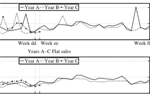
Week cc Week dd Week ee Week ff Years A−C Sales
Year A Year B Year C
Week cc Week dd Week ee Week ff Years A−C Flat sales
Year A Year B Year C
Figure 1: Comparison of real sales with flat sales per year
Neuro-fuzzy modeling, refers to the way of applying various learning techniques developed in the neural network literature to fuzzy modeling or a fuzzy inference system. ANFIS use a feed forward network to search for fuzzy decision rules that perform well on a given task. Using a given input-output data set, the system creates a FIS whose membership function parameters are adjusted using a back-propagation algorithm alone or a combination of a back-propagation algorithm with a least-squares method.
III. PREPROCESSING OF SALES DATA
One of the goals when building prediction models is the ability to use them on the prediction of several different peri-ods. For that, they need to be sufficiently generic and its inputs robust enough so they can translate the system’s dynamics effectively. For this purpose, it’s necessary that the inputs are constructed in a coherent manner with a logic that sustains the numerical values that they have. Due to confidentiality restrictions none of the timespan can be associated to real years, months or specific days (such as known holidays). A. Period definition
For the period definition, the available data in a first approach was weekly sales data form weekaato weekaa+44, named f f from year A to B, and from week aa to week
aa+ 22, named ee, of year C. The objective of this work is forecasting year C sales. For that purpose, the models are trained using data from a certain period of year A andB to predict the same period of year C. After defining the periods of forecasting, daily sales data is used in the modeling and forecasting phase.
The approach chosen to deal with period selection was to select three different forecasting periods, starting from a stationary period (no disturbances) and evolving to gradually more complex (disturbed) periods. The stationarity of a sales curves means a sales pattern without the effect of monthly seasonality, yearly seasonality and promotions. In Fig. 1 is presented the comparison between the real weekly sales curve with the flat curve, without the previous effects. From this figure is possible to compute the three forecasting periods desired. As the real curve from weeks aatobbhas a similar dynamic than the flat, it means that it’s a period without major events and, thus, stationary. If we extend the period to weeks ccthere is an inclusion of some disturbances to this
TABLE I: WEEKLY SEASONALITY Week day Mon Tue Wed Thu Fri Sat Sun
ws 0 -0.1 -0.2 -0.12 0 1 0.8
period. Furthermore, if the period is even more extended until weeksdd, it is defined a period plenty of disturbances, which dynamics are translated by a non-stationary behavior instead of a stationary with disturbances behavior. In this sense, the periods are defined as:Stationary period:From weeksaato
bb, 6 weeks, 42 days per year, 126 days in total; stationary period with disturbances: From weeks aa to cc, 9 weeks, 63 days per year, 189 days in total; non-stationary period: From weeksaatodd, 20 weeks, 140 days per year, 420 days in total.
B. Feature construction
The goal of feature construction is to obtain features that accurately represent the effects that they have in sales. For that, one needs to understand its effect, and then have a logical approach to its mathematical definition. The main attributes that influence sales are theweekly seasonality (ws),monthly seasonality (ms), purchasing power of customers (pw), promotions (p) andholidays or festive days (h).
1) Weekly seasonality (ws): The weekly seasonality could be compared to a distribution of sales during the week. It is a pattern that describes sales during the several days of the week. There is a peak on weekend sales, which starts to raise from wednesday, and declines until tuesday.
The input started to be constructed as a normalized [0 1] distribution, being saturday 1 and wednesday 0, but after some adaptations, the input resulted as presented in Table I. These adaptations were done based on a greedy heuristic, developed for this feature. As it is a pattern that will remain constant, unless significant political measures occur, such as saturdays become working days as well, which may happen; this type of seasonality will have minor changes through the years. The resulting input is presented on the following table.
2) Monthly seasonality (ms): The monthly seasonality refers to the way people spend money during a month period. Being used to receive wages at the end of the month, usually the last weekend of a month and the first weekend of the next (weekends after wages - WAW) are the weekends where customers are more willing to spend. There is also an addition to this trend, as in the weekend before customers receive their wages (weekend before wages - WBW) they have less money, which has the consequence of being less willing to spend money. So there is contention of expenses and sales on those weekends tend to be lower than on a regular weekend.
The values given to this type of seasonality are represented on Table II, presented next. The logic behind its construction was the multiplicative effect these days have on sales. It was built comparing the values of sales on the intended weekends with the average of a regular weekend. The first group of numbers concerns to the weekend of contention of expenses, and the last to the expected increase in sales.
TABLE II: MONTHLY SEASONALITY
WBW WAW
Sat Sun Sat Sun ms 0.94 0.76 1.27 1.05
3) Purchasing power of costumers (pw): From daily sales analysis, it was clear that despite different years having the same pattern, there was an offset between the curves, where sales have been decreasing along the years.
In that sense it was needed to construct an input that would account for this influence. It was named purchasing power, although it doesn’t have a direct relation with the purchasing power definition, and the goal was to build a vector of inputs, which values would be constant during each year, relating years B and C overall sales behavior with year A. In that sense, the input for year A was zero. Its construction was made through the analysis of internal documentation for the years A and B (10%), and assumed for the forecasting year (26% from yearA toC).
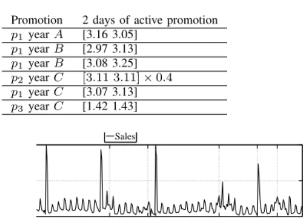
4) Promotions (p): Concerning the promotions, there are of three types. Type 1 (p1) are transversal promotions discounts
spendable in future sales that last 2 or 3 days. There are several of this type of promotions in every year. Type 2 promotions (p2) only happened once in year C, the forecasting year.
The difference is that, instead of the transversal discount, the customer has to spend multiples of a certain amount to have access to the same discount. The third type of promotions, named promotions of type 3 (p3), are promotions equal to p1 but only applied to a category (a part) of a business unit,
instead of being transversal. There is also only one promotion of this type, in yearC. This type of promotions is announced two days before its beginning in order to reduce the decrease on sales that happens in between.
The approach for the construction of this parameter was similar to the monthly seasonality. It was compiled the sales value of the peaks of the promotion compared to the average of the corresponding regular weekday (without the effect of promotions) sales. The value computed was the multiplicative factor in sales due to promotions compared to the same regular weekday. This procedure was also adopted in the 2 days before promotions. In that way, the input for the type 1 promotions,
p1, was constructed as a vector of ones, with the values of
Table III whenever there was a promotion. The p1 present in
the forecasting period is slightly different, as consists of 3 days, where the first is a holiday, and the last is a holiday where people tend to spend in family as is described in the next section. Due to that it was modeled as a 2 day promotion on friday and saturday. The definition of the p2, the first in
the prediction period, was slightly different. Although the type of discount was similar, this promotion lasted for a week, in opposition to the type 1 and 3. The approach taken was to compute the average increase in sales of all days of the type 1 promotion, i.e., the average of all the values of corresponding to the training set in Table III. By doing this, the average effect of ap1was computed. Then the attribute was constructed with
40% (due to an assumed expectation of lower affluence) of this value for all days of promotion. The type 3 promotion,
p3, was modeled in a slightly different way. The effect of the
average increase of a p1 promotion were multiplied by 0.2,
TABLE III: PROMOTION INPUT Promotion 2 days of active promotion p1yearA [3.16 3.05] p1yearB [2.97 3.13] p1yearB [3.08 3.25] p2yearC [3.11 3.11]×0.4 p1yearC [3.07 3.13] p3yearC [1.42 1.43] h3−A h1−B h2−B h3−B h1−C h2−C h3−C Sales
Figure 2: Events related with holidays
TABLE IV: TYPE1EFFECT Year Monday Tuesday (event day) Wednesday
A 1.37 1.33 1.51
B 1.14 1.22 1.01
C 1.26 1.28 1.25
the expected value of the weight of the category in discount in the days of promotion. In that sense, the resulting input of this promotion would be p3 = [1 + (p1−1)×0.2]. Next is
presented Table III, which shows the input values.
5) Holidays or festive days: Finally, the last effect taken in account was the existence of holidays or festive days. These are of three types: a holiday always on the same day of the week,h1; acombination of two holidays, on friday and sunday,
which affect the hole previous week, h2; and a combination
of two holidays always on the same day (different days of the week in different years),h3. In Fig. 2 are represented all the
effects related with this input.
Type 1: In fact, this event is not a holiday (H), it’s a day where employees are allowed to skip work. Due to that, it might implicate going to a major commercial surface and being exposed to the retailer products. From Fig. 2 observation, the main effect is avoiding the sales decrease, delaying the regular week dynamics. In that sense it was compiled using the multiplicative effect this input has on the weekday and its neighborhood of the event. The values are presented in Table IV.
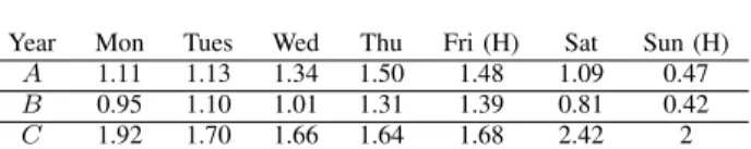
Type 2: This type of holidays is a combination of 2 holidays but has an effect on a hole week. It is period marked by contention due to the facts associated with it. The week ends with holidays on friday and sunday. Specially on sunday, families tend to gather and spend the day together. Being an important holiday, in years A and B, stores were only partially opened (half day), which had the consequence of lowering sales in those days. Although sunday is an important day, the hole week has a different behavior. As before, the rational behind the definition of the hole week as input, was the quotient between sales those days and average sales for the same weekday, without promotions effect. The prediction input was slightly different, as it wasn’t the average of the effect on
TABLE V: TYPE2EFFECT
Year Mon Tues Wed Thu Fri (H) Sat Sun (H)
A 1.11 1.13 1.34 1.50 1.48 1.09 0.47
B 0.95 1.10 1.01 1.31 1.39 0.81 0.42
C 1.92 1.70 1.66 1.64 1.68 2.42 2
the previous years for one of the days. In year C there was a
p1on the weekend, beginning on friday and ending on sunday,
which means that stores weren’t partially closed on sunday. In that sense, for this day, as the previous years shape a partially closed day, the input was as if there was no effect, as if it was a regular sunday. This approach was chosen for two reasons. Firstly, it’s impossible to know the effect of a open sunday holiday, as the data doesn’t show it. Secondly, there is a p1
promotion on that weekend and sunday was the last day of promotion, which may be sufficient to counter the possible decrease that a sunday holiday of this type may have in sales. In that sense, the input is presented in Table V. This approach was already mentioned for the promotions.
Type 3: This is an effect cause by a combination of two holidays. This holidays have 5 days in between, which means that they form a week if the days between are considered, which was the case. The approach used to build this attribute was similar to the remaining, having some minor changes.
In yearsAandBboth holidays have a completely different behavior, which makes the definition of this attribute very difficult to accomplish. This has concern to politics in the company as well because, as in the Type 2 holidays, where shops closed on sunday afternoon in year A andB and then were opened in year C; here, for instance, on the holiday of the end of the week of yearAshops did close on the afternoon (sales break down), whereas in years B and C they were opened. Also, the first holiday of the week in year B was the day right after the Type 2 sunday (holiday), when shops closed in the afternoon, leading to an increase in sales.
In addition to these facts, both holidays have a fixed day, which, in comparison with Type 1 and 2, is worse for input construction, because it means that they move around week-days during the years. And, as it was possible to see throughout the section, sales have a high dependence on weekdays, and the fact that these holidays change their weekday depending on the year, makes defining its influence through training very difficult.
The procedure to the construction of this input was to define a quotient between the multiplicative effect on sales each day. The only points that were not averaged, were the ones where in one of the years was a promotion (yearB) and where the stores were partially closed (year A). Those values were chosen to be the same as the year A values, in the first case; and the same as the values in yearB, in the second case. Finally, as there was intense promotional activity in that week, those values were multiplied by 2. Table VI presents the input vales.
IV. INTELLIGENT MODELING FOR SALES FORECASTING After developing the inputs, the models were obtained. There were five models applied to each forecasting horizon:
TABLE VI: TYPE3HOLIDAYS INPUT
Year Day1(H) Day2 Day3 Day4 Day5 Day6 Day7(H)
A 0.91 0.88 0.88 0.91 1.05 1.21 0.65
B 1.01 0.83 0.78 0.73 0.62 3.08 3.25
C 0.96 0.85 0.83 0.82 0.84 1.21 1
Fuzzy classification models,fuzzy NARX models (FNARX), feedforward classifications neural networks, NARX net-works (NNNARX) and ANFIS. Each model was trained using the pervious section’s periods and inputs. Concerning the fuzzy models, different cluster (C) structures were compared and different delays for the NARX. For neural networks different combinations of hidden-layers (HL) and neurons (N) were balanced, and different delays for the NARX. For the ANFIS, only in one period different numbers of membership functions (MF) were analyzed, as for the longer periods, due to computational efforts, it was only possible to perform with 2 MF.
For the fuzzy models, the fuzziness exponent was set to 2; the termination tolerance to0.01; the seed tosum(100∗clock); the antecedents were antecedent membership functions and the consequents estimated with locally weighted Least-Squares. The clustering algorithm was chosen to be the Fuzzy C-means. For the neural networks, the number of training epochs and training algorithm used were 1000 training epochs and Levenberg-Marquardt algorithm, respectively. For the AN-FIS, the number of training epochs was set to 20 and the membership functions used were Gaussians. A summary of the parameters for all the models in each specific period, is resented in Table VII. For the stationary period the delays in the FNARX an NNNARX were of [7,1,3,4] and [11 for all] for the [s,ws,ms,pw] inputs, respectively. Concerning the stationary period with disturbances, the delays were of [9,3,5,1,3,1] and [11 for all] for the [s,ws,ms,pw,h,p] inputs, respectively. For the last period, it was of [7,1,5,1,14,1] and [10 for all] for the [s,ws,ms,pw,h,p] inputs, respectively.
V. RESULTS AND DISCUSSION
This section is divided by forecasting period and only the best forecast is presented in a figure. The performance criteria used were the variance accounted for, V AFi = (
1−var(yi−yˆi)
var(yi)
)
×100%; and the root mean square error,
RM SE=
√∑n
i=1(x1,i−x2,i)2
n .
A. Stationary period
The models’ performance for the stationary period are pre-sented in Table VIII and the best model forecast is prepre-sented in Fig. 3. As it is possible to observe in Fig. 3 and Table VIII, the fuzzy classification model, which had the worse performance of all the models in training, presents the best test results. The main differences between the forecast and target are a discrepancy in the beginning of the period, some irregular peaks during weekdays and a general offset between both curves. The first may have to due with a discounts season that usually happens in that season but, as can be seen in previous years, that effect is’n visible and wasn’t shaped in testing due to the lack of importance. The majority of the
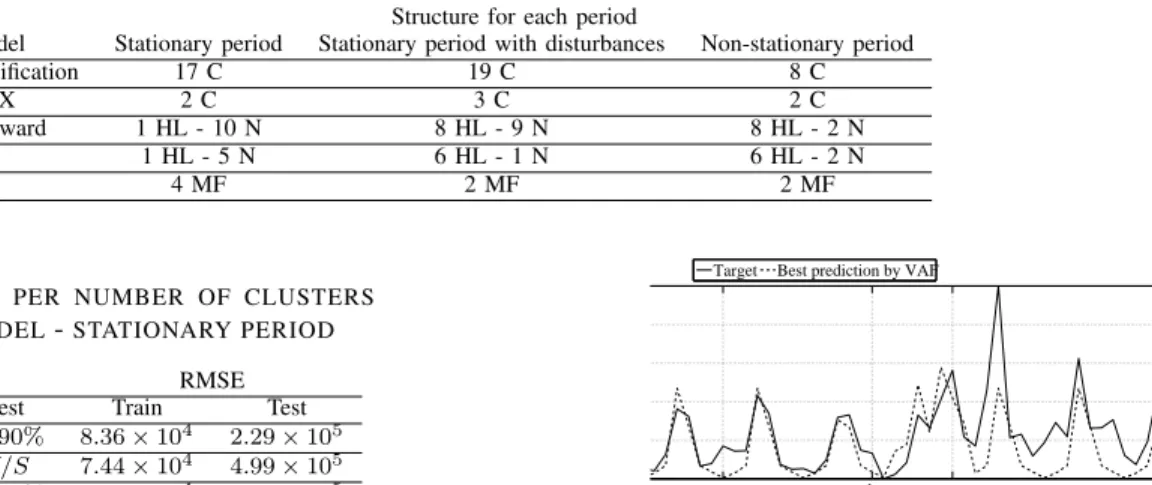
TABLE VII: PARAMETERS OF THE MODELS FOR EACH PERIOD Structure for each period
Type of model Stationary period Stationary period with disturbances Non-stationary period
Fuzzy Classification 17 C 19 C 8 C
Fuzzy NARX 2 C 3 C 2 C
NN Feedforward 1 HL - 10 N 8 HL - 9 N 8 HL - 2 N
NN NARX 1 HL - 5 N 6 HL - 1 N 6 HL - 2 N
ANFIS 4 MF 2 MF 2 MF
TABLE VIII: PERFORMANCE PER NUMBER OF CLUSTERS FOR THE CLASSIFICATION MODEL-STATIONARY PERIOD
VAF RMSE
Model Train Test Train Test
Fuzzy Class. 91.16% 84.90% 8.36×10⁴ 2.29×10⁵ Fuzzy NARX. 92.60% N/S 7.44×10⁴ 4.99×10⁵ Feedforward NN 91.79% 48.83% 8.02×10⁴ 3.64×10⁵ NARX NN 67.67% 59.93% 1.81×10⁵ 2.64×10⁵ ANFIS Class. 92.30% 81.31% 7.84×10⁴ 1.50×10⁵ a b
Target Best prediction by VAF
Figure 3: Sales forecasting with the fuzzy classification model - Stationary period
TABLE IX: PERFORMANCE PER NUMBER OF CLUSTERS FOR THE CLASSIFICATION MODEL - STATIONARY PERIOD WITH DISTURBANCES
VAF RMSE
Model Train Test Train Test
Fuzzy Class. 95.64% 54.42% 1.06×10⁵ 2.41×10⁵ Fuzzy NARX. 96.26% N/S 9.02×10⁴ 3.08×10⁵ Feedforward NN 60.42% N/S 3.77×10⁴ 2.82×10⁶ NARX NN 19.05% N/S 3.40×10⁵ 3.95×10⁵ ANFIS Class. 96.13% N/S 9.55×10⁴ 3.85×10⁵
effects on the middle of the week seem random, although point a is precisely the beginning of the month. In that sense, it could be introduced as input. But from training data, this effect is not visible, thus, it wouldn’t be expected to happen. Point b is also an exception as it was a special day that wasn’t accounted due to the fact that in the only year that this effect was visible was coincident with the h1 promotion.
B. Stationary period with disturbances
The models’ performance for the stationary period with disturbances are presented in Table IX and the best model forecast is presented in Fig. 4. The only model that performed well enough was, once again, the fuzzy classification model In Fig. 4 is possible to observe that the lower performance has to due with the added weeks, where there are several effects that couldn’t be captured by the system. Thep2promotion (poinsb
a b c
Target Best prediction by VAF
Figure 4: Sales forecasting with the fuzzy classification model - stationary period with disturbances
TABLE X: PERFORMANCE PER NUMBER OF CLUSTERS FOR THE CLASSIFICATION MODEL-NON-STATIONARY PERIOD
VAF RMSE
Model Train Test Train Test
Fuzzy Class. 92.98% 64.41 1.82×10⁵ 3.15×10⁵ Fuzzy NARX. 92.35% N/S 1.47×10⁵ 4.58×10⁵ Feedforward NN 47.97% N/S 3.49×10⁵ 4.75×10⁵ NARX NN 5.48% N/S 5.16×10⁵ 1.51×10⁶ ANFIS Class. 93.28% N/S 1.61×10⁵ 8.05×10⁵
toc) is badly captured, only the part aligned with theh1(point
(c)) is minimally accurate. The biggest error comes after, on the final weeks of the period where no event is defined, due to the fact that on the training set none happens on those weeks in previous years.
C. Non-stationary period
The models’ performance for the non-stationary period are presented in Table X and the best model forecast is presented in Fig. 5. In this period, the best model was, once again, the fuzzy classification system. The higher VAF of this period’s forecast means that the addition made to this period has a better forecast than the one presented in the stationary period with disturbances. In fact, the model presents the same failures as the stationary and stationary with disturbances period, in what capturing the system dynamics is concern. In addition to that, it has also some difficulties in capturing eventh3, which
was already expected. Theh2effect is not possible to discuss
due to a combination of that event withp1, which the system
was able to capture accurately. Concerning thep1 andp3, the
system is extremely accurate on its forecast. Concerning the
p1, and comparing with the retailer’s forecast (the only type
of forecast made by the retailer), is important to mention that the model had an error of 1.7% of the total promotion, while the retailer had an error of 30%. This is a major improvement.
b c h2 & p1 h3 p3 Target Best prediction by VAF
Figure 5: Sales forecasting with the fuzzy classification and NARX model - Non-stationary period
VI. CONCLUSION
This work addressed the problem of sales forecasting, by applying soft, or intelligent, computing techniques to a retailer. Firstly, the approach to the problem was defined, selecting the periods to forecast and which features to use in each period. Then, different modeling techniques were applied and the models for each technique were obtained. Finally, the forecasting results were achieved for each horizon of prediction.
For the five models applied to the problem, only the fuzzy classification is applicable to the problem, achieving accurate forecasts of the stationary trend and some well defined events. Specially for the stationary period, the performance was superior than for the remaining periods. The remaining models are not applicable.The reasons for not having performances as high as on the first period have to due with exceptional events that either weren’t present in training data and, therefore the model couldn’t learn its impact; or were present in training but not in the way as it happened in the test year. So, although the model had knowledge about the impacts of these events, it didn’t had knowledge about the precise circumstances in which these events would affect the system. The first examples are, for instance, the three weeks after the p2 promotion, where
there is an increase in sales and, on previous years, that didn’t happen and it wasn’t predictable to happen in year C. It is also the case of thep2promotion, which is a promotion never
made before. For the second case there is the week of the
h3 holidays, when although there was knowledge about past
years, the fact that these holidays are movable, in addition with a strong promotional activity made this events unpredictable. On the other hand, one major conclusion that can be drawn is the accurate forecast of thep1 andp3promotions. On the two
promotions of this type in testing, the sales value estimations were very accurate.
Finally, an important conclusion is that the best model improves by far the actual forecasting existing in the company analyzed. In the future, this tool can bring major benefits.
ACKNOWLEDGEMENTS
This work was supported by Strategic Project, ref-erence PEst-OE/EME/LA0022/2011, through FCT (under the Unit IDMEC - Pole IST, Research Group ID-MEC/LAETA/CSI). This work is also supported by the FCT grant SFRH/BPD/65215/2009, Fundac¸˜ao para a Ciˆencia e a Tecnologia, Minist´erio da Educac¸˜ao e Ciˆencia, Portugal. The authors would also like to thank SONAE SR and more specifi-cally Eng. Hugo Alexandre and his team, for providing all the
information needed and for all the support given throughout the project.
REFERENCES
[1] F. Chen and T. Ou, “Sales forecasting system based on gray extreme learning machine with taguchi method in retail industry,”Expert Systems with Applications, vol. 38, no. 3, pp. 1336 – 1345, 2011.
[2] I. Alon, M. Qi, and R. J. Sadowski, “Forecasting aggregate retail sales: A comparison of artifcial neural networks and traditional methods,” Journal of Retailing and Consumer Services, pp. 147–156, 2001. [3] T. Xiao and X. Qi, “Price competition, cost and demand disruptions
and coordination of a supply chain with one manufacturer and two competing retailers,”Omega, vol. 36, no. 5, pp. 741 – 753, 2008. [4] A. A. Levis and L. G. Papageorgiou, “A hierarchical solution approach
for multi-site capacity planning under uncertainty in the pharmaceutical industry,”Computers and Chemical Engineering, vol. 28, no. 5, pp. 707 – 725, 2004.
[5] G. E. P. Box and G. Jenkins,Time Series Analysis, Forecasting and Control. Holden-Day, Incorporated, 1990.
[6] S. W. Makridakis, S. and V. McGee,Forecasting: Methods and Applica-tions, 2nd edn. New York, NY, USA: John Wiley & Sons, Chichester, 1983.
[7] A.-C. Cheng, C.-J. Chen, and C.-Y. Chen, “A fuzzy multiple criteria comparison of technology forecasting methods for predicting the new materials development,”Technological Forecasting and Social Change, vol. 75, no. 1, pp. 131 – 141, 2008.
[8] C.-W. Chu and G. P. Zhang, “A comparative study of linear and nonlinear models for aggregate retail sales forecasting,” International Journal of Production Economics, vol. 86, no. 3, pp. 217 – 231, 2003. [9] M. J. C. Hu, “Application of the adaline system to weather forecasting,”
E. E. Degree Thesis, Stanford Electronic Lab, Tech. Rep., 1964. [10] G. Zhang, B. E. Patuwo, and M. Y. Hu, “Forecasting with artificial
neu-ral networks:: The state of the art,”International Journal of Forecasting, vol. 14, no. 1, pp. 35 – 62, 1998.
[11] J. Deppisch, H.-U. Bauer, and T. Geisel, “Hierarchical training of neural networks and prediction of chaotic time series,”Physics Letters A, vol. 158, no. 1 - 2, pp. 57 – 62, 1991.
[12] E. M. Azoff, Neural Network Time Series Forecasting of Financial Markets, 1st ed. New York, NY, USA: John Wiley & Sons, Inc., 1994.
[13] D. Srinivasan, A. Liew, and C. Chang, “A neural network short-term load forecaster,”Electric Power Systems Research, vol. 28, no. 3, pp. 227 – 234, 1994.
[14] J. Su´arez, O. Mayora-Ibarra, J. Torres-Jim´enez, and L. Ruiz-Su´arez, “Short-term ozone forecasting by artificial neural networks,” Advances in Engineering Software, vol. 23, no. 3, pp. 143 – 149, 1995. [15] S. Y. Kang, “An investigation of the use of feedforward neural networks for forecasting,” Ph.D. dissertation, Kent, OH, USA, 1992, uMI Order No. GAX92-01899.
[16] Z. Tang and P. A. Fishwick, “Feedforward neural nets as models for time series forecasting,”INFORMS Journal on Computing, pp. 374– 385, 1993.
[17] J. M. P. Menezes, Jr. and G. A. Barreto, “Long-term time series predic-tion with the narx network: An empirical evaluapredic-tion,”Neurocomput., vol. 71, no. 16-18, pp. 3335–3343, Oct. 2008.
[18] P. Dash, A. Liew, S. Rahman, and S. Dash, “Fuzzy and neuro-fuzzy computing models for electric load forecasting,” Engineering Applications of Artificial Intelligence, vol. 8, no. 4, pp. 423 – 433, 1995.
[19] A. Al-Anbuky, S. Bataineh, and S. Al-Aqtash, “Power demand predic-tion using fuzzy logic,”Control Engineering Practice, vol. 3, no. 9, pp. 1291 – 1298, 1995.
[20] R. Kuo, P. Wu, and C. Wang, “An intelligent sales forecasting system through integration of artificial neural networks and fuzzy neural networks with fuzzy weight elimination,” Neural Networks, vol. 15, no. 7, pp. 909 – 925, 2002.
[21] P.-C. Chang, Y.-W. Wang, and C.-H. Liu, “The development of a weighted evolving fuzzy neural network for pcb sales forecasting,” Expert Systems with Applications, vol. 32, no. 1, pp. 86 – 96, 2007.