中央研究院經濟所學術研討論文
IEAS Working Paper
On the Budget-Constrained IRS : Equilibrium and Efficiency
Meng-Yu Liang and C.C. Yang
IEAS Working Paper No. 07-A002
January, 2007 Institute of Economics Academia Sinica Taipei 115, TAIWAN http://www.sinica.edu.tw/econ/
中央研究院
經濟研究所
I
NSTITUTE
OF
E
CONOMICS,
A
CADEMIA
S
INICA
TAIWAN
copyright © 2006 (Meng-Yu Liang and C.C. Yang)On the Budget-Constrained IRS: Equilibrium and
E¢ ciency
Meng-Yu Liang
Institute of Economics, Academia Sinica, Nankang, Taipei 115, Taiwan
C.C. Yang
Institute of Economics, Academia Sinica, Nankang, Taipei 115, Taiwan
Department of Public Finance, National Chengchi University, Wenshan, Taipei 116, Taiwan
Abstract
This paper extends Graetz, Reinganum and Wilde’s (1986) seminal work on tax compliance to the real-world scenario where the IRS (Internal Revenue Service) faces a budget constraint imposed upon her by the Congress. The paper consists of two parts. The …rst part is positive – we characterize the equilibria resulting from the interaction between taxpayers and the budget-constrained IRS. The second part is normative – we examine the e¢ ciency implication of varying the size of the budget allocated to the IRS. It is shown that, to mitigate or eliminate the so-called “congestion e¤ect,” the IRS should be su¢ ciently budgeted and, in particular, we provide a case for the policy prescription that the size of the budget allocated to the IRS should be expanded as
Corresponding author, C.C. Yang. Mailing address: Institute of Economics, Academia Sinica, Nankang, Taipei 115, Taiwan. Email: [email protected]
long as an additional dollar allocated could return more than an additional dollar of tax revenue.
1
Introduction
“Unlike other government agencies, there is a positive return on money invested in the IRS. ... In its FY2007 budget recommendation, the Board calls for a modest increase in enforcement that would result in a real return on investment, ranging from three to six dollars on every dollar spent, resulting in $730 million revenue increase by FY2009 on a $242 million investment.”
IRS Oversight Board (2006, pp. 12-13)1
On the basis of a 3-1 to 6-1 return for an additional dollar invested, does it make sense for the Board to recommend an expanded IRS budget on enforcement? This paper provides a case for the positive answer.
We consider a model of tax compliance, which extends the seminal work of Graetz, Rein-ganum and Wilde (1986, hereafter GRW) to the real-world scenario where the IRS faces a budget constraint imposed upon her by the Congress. The paper consists of two parts. The …rst part is positive. We characterize the equilibria resulting from the interaction between taxpayers and the budget-constrained IRS, and study the impact of imposing budget con-straints on the IRS. The second part is normative. We examine the e¢ ciency implication of varying the size of the budget allocated to the IRS and, in particular, we ask: how much should we fund the IRS?
Unlike the classical work of Allingham and Sandmo (1972) and Yitzhaki (1974) on tax evasion, which treats the IRS actions as exogenous, the GRW model views the IRS as a
1“The IRS Oversight Board was created by the IRS Restructuring and Reform Act of 1998 (RRA 98),
which was enacted to improve the IRS so that it may better serve the public and meet the needs of taxpayers.” (see the web-site of the Board)
strategic player that interacts with taxpayers. The GRW model also di¤ers from the principal-agent tax evasion model …rst introduced by Reinganum and Wilde (1985). As pointed out by GRW, the principal-agent model su¤ers from the time inconsistency problem since it requires that the IRS announce and commit to an audit policy, even though the precommitted audit policy will typically prove suboptimal once taxpayers submit their reported income. GRW emphasize that their interactive model follows the natural temporal sequence of decisions: …rst, taxpayers report their income, and only then does the IRS decide whether to perform tax audits.2
Graetz, Reinganum and Wilde (1984, hereafter GRW0) also extend the GRW model to
account for the e¤ect of imposing budget constraints on the IRS. However, their way of deriving equilibria is somewhat complicated. We believe our approach greatly simpli…es the analysis. More importantly, we further address the e¢ ciency issue across equilibria whereas they do not. We will compare our approach with the GRW0 approach after we derive the
equilibria of our model.3
Slemrod and Yitzhaki (1987) investigate the same normative question as our paper. The main di¤erences in modeling include: (i) while they study tax auditingwith commitment, we study tax auditingwithout commitment; and (ii) while they subsume the IRS and the Congress under the rubric of a single player called “government,” we treat the IRS and the Congress as two di¤erent players. Perhaps more interestingly, the policy prescription derived from our model starkly contrasts that derived from their model. Slemrod and Yitzhaki prescribe
2For recent surveys of the tax evasion literature, see Andreoni et al (1998), Slemrod and Yitzhaki (2002),
Cowell (2004) and Sandmo (2005). Auditing is typically a negative-sum game between taxpayers and the IRS. However, using auditing as a threat, it may be feasible for the IRS to create a Pareto-improving outcome for both taxpayers and the IRS under some circumstances; see Chu (1990) and Ueng and Yang (2000, 2001) for the details.
3Macho-Stadler and Perez-Castrillo (1997) consider the e¤ect of imposing budget constraints on the IRS
that the size of the budget allocated to the IRSshould not be expanded to the level where an additional dollar allocated would return just an additional dollar of tax revenue.4 By contrast,
we prescribe that the size of the budget allocated to the IRS should be expanded until an additional dollar allocated would return just an additional dollar of tax revenue. It is shown within our model that our policy prescription always dominates other policy prescriptions that fall short of equating the marginal revenue to the marginal cost of tax collection. The dominating criterion is based on the lower e¢ ciency cost per dollar of tax collection. We will make more comparisons between our result and theirs when we address the e¢ ciency issue.
The remainder of this article is organized as follows. Section 2 describes the basic model. Section 3 provides the full characterization of the equilibrium outcomes. Section 4 addresses the e¢ ciency issue and provides an answer to the optimal funding of the IRS. Section 5 considers an extension of the basic model and Section 6 concludes.
2
Basic Model
Our basic model is essentially the same as the GRW model. For ease of exposition, however, we transform the GRW model into an equivalent, but simpler, model. GRW assume that taxpayers earn either high or low income. High-income taxpayers need to pay a high tax, while low-income taxpayers need to pay a low tax. We normalize the low income of the GRW model to zero so that either taxpayers earn an income or they do not. Only the taxpayers who earn the income need to pay tax in our model. GRW defend their simple setup by arguing that “the model might also be viewed as addressing issues of noncompliance across a
4This conclusion is also drawn by Usher (1986), Kaplow (1990), Mayshar (1991), and Sanchez and Sobel
(1993). A feature of the Slemrod-Yitzhaki model that these papers have in common is the auditing with commitment. Except for the principal-agent model of Sanchez and Sobel (1993), these papers, similar to Slemrod and Yitzhaki (1987), subsume the IRS and the Congress under the rubric of a single player called “government.”
relatively small range of income–for example, within a given audit class”(GRW, p. 17). We consider an extended model with multiple audit classes in Section 5.
Suppose that there is a unit mass of continuum taxpayers who may earn an incomey >0. This income need not be the total income earned. It may simply represent a particular type of income, say, income from vehicle sales or tip income. Those taxpayers who have incomey
are obliged to pay a positive taxT (< y), while those who do not have y are obliged to pay nothing. The IRS knows that there is a q 2 (0;1) portion of taxpayers who have y, and a
1 q portion of taxpayers who do not have y. However, the IRS cannot identify a priori which taxpayer has y and which taxpayer does not havey. As emphasized by GRW, one of the distinct features of modern systems of income taxation is their self-reporting nature: the tax law requires taxpayers to …le tax returns and report their own income to the IRS. The taxpayers who do not haveywill always report nothing to the IRS truthfully. However, some taxpayers who haveymay cheat and also report nothing. A cheater is subject to a …neF >0
if he is discovered cheating by the IRS. This …ne is imposed in addition to the taxT due with
T+F y(the limited liability constraint). The taxpayers who haveyare assumed to possess a common von Neumann-Morgenstern utility function over income, namely,u:R+ !R+ with u0 >0 and u00 < 0. They maximize the expected utility by choosing to report y or report
nothing.5
After receiving a taxpayer’s report, the IRS can decide whether to perform an investigative tax audit. Auditing is costly and the IRS has to bear a cost ofc >0 to verify each taxpayer. We assume as in GRW that the truth will be discovered once a tax audit is performed and
5There are the so-called “ghost” taxpayers, who fail to …le their tax returns to the IRS as required by the
tax law (Cowell and Gordon, 1995; Erard and Ho, 2001). In our simple model, those taxpayers who havey
but report nothing to the IRS and those taxpayers who havey but do not report it to the IRS can be treated as the same. Thus, there are two possible interpretations for non-compliance in our model: (i)underreporting
if taxpayers havey but report nothing to the IRS, and (ii)non-…ling if taxpayers have y but fail to …le tax returns with the IRS.
that it always pays o¤ for the IRS to audit an evader (i.e. T +F > c). Under a given budget constraintI, the IRS’s objective is to maximize the tax revenue collected (including taxes and …nes), net of audit costs through auditing. Because auditing is costly, it is clear that the “pro…t-maximizing” IRS will only audit those taxpayers who report nothing. We assume that none of the taxpayers bear any additional cost during the auditing process. We also assume that the IRS cannot use the taxes or …nes collected to …nance her own auditing expenses.6 The IRS takes the tax T , the …ne F and the budget I as given in her auditing
since these variables are predetermined by the Congress. Our focus is on the impact ofI.7
The timing of this game is as follows. Given the realization of y ; c; T; F and I, those taxpayers who do not have y always report nothing, and those taxpayers who have y simul-taneously choose whether to report y or not. After observing the taxpayers’ reports, the IRS randomly chooses to audit a fraction of taxpayers who do not report y. We solve the equilibrium of this game under the condition that the IRS’s strategies are restricted to depend on the distribution of the taxpayers’reports only.8
3
Equilibrium
3.1
Equilibrium outcomes
In this subsection we will characterize all the equilibrium outcomes of the game.
6Wertz (1979, p. 144) describes the rule of the game: “An agency [the IRS] may not spend more on
enforcement activities in a budget period than its legislature has appropriated for them. De…ciencies collected throughout the period are transmitted to the general government; they may not be used by the agency to expand its activities.”
7Both the taxT and the …neF are also under the control of the Congress. However, their determination
is not on the yearly basis as the budgetI.
8This restriction implies that a unilateral deviation by a single taxpayer cannot in‡uence the course of our
3.1.1 Characterization
We use the notation to denote the portion of cheaters among all taxpayers,9and the notation
( )to denote the IRS’s best audit response to . It is clear that 2[0; q]and ( )2[0;1]. Note that the IRS can observe in our model. This is because the IRS knows by assumption that there is aq2(0;1)portion of taxpayers who havey, but only aq portion of taxpayers report havingy to the IRS.
For any 2[0; q], letR( )denote the IRS’s (gross) expected revenue from a single audit. Thus,
R( ) =
+ (1 q)(T +F)
where + (1 q) is the portion of taxpayers who do not report y. R( ) represents the marginal revenue of tax collection to the IRS when there is the amount of cheaters. Observe that R(0) = 0; R(q) = q(T +F), and @R@ >0.
To characterize the equilibrium, we need to de…ne several other notations. First, de…ne as the probability of audit such that a taxpayer who has income y is merely indi¤erent between reportingy and not reporting y. That is,
u(y T F) + 1 u(y) =u(y T):
Secondly, de…ne as the amount of such that the IRS is merely indi¤erent between auditing and not auditing. That is,
R( ) =c: (1)
Finally, de…ne ^ as the amount of such that the IRS uses as the audit probability and
9Thus, the portion of honest taxpayers (including those who haveyand also reportyto the IRS, and those
who do not havey) equals(q ) + (1 q) = 1 . Note that the notation in the GRW model denotes the portion of actual cheaters among those who arepotential cheaters, while it denotes the portion of cheaters
just exhausts all her budget. That is,
( ^ + 1 q)c=I:
For convenience, we shall call “the taxpayer who hasy”simply “the taxpayer”from now on. We use( ; )to denote the outcome of an equilibrium. Let be the set of all equilibrium outcomes. The following proposition characterizes the set of equilibrium outcomes of the game.10
Proposition 1 (i) If R(q)2[0; c), then =f(q;0)g. (ii) If R(q) = c, then = f(q; ) : 2[0;minfIc; g]g. (iii) If R(q)> c, then
a) =f(q; I
c)g for I 2[0; ( + 1 q)c);
b) =f( ; ); ^; ; q;cI g for I 2[ ( + 1 q)c; c];
c) =f( ; )g for I 2( c, 1).
Remark 1 In b) of Proposition 1 (iii), ^; will coincide with( ; )if I = ( + 1 q)c,
while it will coincide with q;Ic if I = c. This can be seen directly from the de…nition of ^.
Remark 2 Taxpayers report their income to the IRS before auditing and, therefore, they are …rst movers in the auditing game. However, unlike the leader in a Stackelberg game, knowing
the IRS’s response ( ) does not help the taxpayers much because no taxpayer can alter by
his single deviation and hence no taxpayer can a¤ect by his income report (remember our
regularity assumption that the IRS’s strategies only depend on the distribution of the taxpayers’ reports). As a result of this “impotent” feature, the taxpayers de facto take the IRS’s audit
probability as given. This explains why the subgame perfect equilibrium coincides with the
Nash equilibrium in our model. This coincidence is consistent with Kalai’s (2004) observation that the equilibria of simultaneous-move games are robust to a large variety of extensive or sequential modi…cations when there are many players.
3.1.2 Hard-to-tax
There are the so-called “hard-to-tax”taxpayers, which is a common referrence to small …rms, smaller farmers, self-employed persons, and informal suppliers.11 These taxpayers could be
de…ned as those whose “tax amounts are quite low compared with the administration costs that would have to be incurred by the tax administration to assess the proper amount of tax.” (Thuronyi, 2004, p. 102). This de…nition corresponds to the case where R(q)2 [0; c]
in our model. “Hard-to-tax” is not the same as “impossible-to-tax” after all. It is simply not pro…table for the IRS to audit these taxpayers. As a result of lacking the motivation to audit, a very high level of evasion results in equilibrium ( =q in Proposition 1 (i) and (ii)). The possibility that the corner solution =q will occur when audit costs are very high has been noted by GRW. Our minor addition is to point out that if the equilibrium outcome
=q is associated with R(q)2 [0; c], then pouring more resources into tax administration will be of little help in resolving the problem and =q will still result. Bird and Casanegra de Jantscher (1992) emphasize that a common constraint usually faced by tax reforms in developing countries is the scarcity of resources for tax administration. This emphasis may need to be quali…ed in light of our …nding here.12
3.1.3 Graphic illustration
The intuition underlying Proposition 1 (iii) is best understood in terms of the best-response graphs of the taxpayers and of the IRS. Figures 1a, 1b and 1c illustrate a), b) and c) of
11Informal suppliers are de…ned as: “individuals who provide products or services through informal
arrange-ments which frequently involve cash-related transactions or ‘o¤ the books’ accounting practice.” (Internal Revenue Service, 1996, p. 43)
12Former IRS Commissioner Lawrence B. Gibbs was reported to have stated that the IRS will not collect
“small amounts owed by such a huge number of taxpayers that collection e¤orts would not be cost-e¤ective” (Los Angeles Times, 1987). Inspired by Gibbs’statement, Reinganum and Wilde (1988) consider a model in which the IRS will tolerate evasion in cases where collection e¤orts would not be cost-e¤ective for the IRS.
Proposition 1 (iii), respectively. In each …gure, the dotted curve represents the taxpayers’ best response while the solid curve represents the IRS’s. Note that taxpayers adopt pure rather than mixed strategies in our model. In drawing the dotted curve, it is assumed that there exists a representative taxpayer who will choose evasion with a probability of q and compliance with a probability of qq . Our pure-strategy outcome is realized through the representative taxpayer’s in…nite trials so that, due to the law of large numbers, the amount of taxpayers will evade while theq amount of taxpayers will comply.
[Insert Figure 1 about here]
Note that the shape of the taxpayers’ best-response curve remains the same as that in GRW. Note also that the shape of the IRS’s best-response curve remains the same as that in GRW if < . However, the shape of the IRS’s best-response curve changes if : Two salient features stand out. First, the result ( )2[0;1]would be true at = if there were no budget constraint. This is because is by de…nition the amount of such that the IRS is indi¤erent between auditing ( = 1) and not auditing ( = 0). However, when the budget constraint is imposed, it may no longer be feasible for the IRS to support any 2 [0;1] as she would wish. Instead, we have ( ) 2 [0;minfc( +1I q);1g] at = . In terms of the graph, the height of the IRS’s best response curve at = may fall short of 1 as shown in Figures 1a and 1b. Secondly, when > , R( ) > c will hold so that an incremental dollar of audit input could return more than an incremental dollar of tax revenue. As a result, the “pro…t-maximizing” IRS would audit for sure if there were no constraint on her budget. That is, ( ) = 1 would hold for all > . This may no longer be true when the budget constraint is imposed. Speci…cally, a binding budget constraint will bring down the feasible probability of audit that the IRS can support and, moreover, the larger the amount of evaders (i.e. a higher ), the lower the probability of audit that these evaders will face (i.e. a lower ). This “congestion”e¤ect, which is emphasized by GRW0, is captured in our model by the downward-sloping part of the IRS’s best response curve as > .
Note that ( ) = I
c( +1 q) for if ( ) 1. This explains the shape of the IRS’s
best-response curve as in Figure 1 (i.e. @@( ) < 0 and @2@ ( )2 > 0). The intersection of the dotted and the solid curve in Figure 1 pins down the equilibrium of the game. There are three intersections in Figure 1b, while there is a single intersection in both Figures 1a and 1c. The former intersections represent the three possible equilibria characterized in b) of Proposition 1 (iii), while the latter intersection represents the unique equilibrium characterized in a) and c) of Proposition 1 (iii), respectively. We shall have more to say on these equilibrium outcomes later.
3.2
Discussion
This subsection discusses several issues related to Proposition 1.
3.2.1 Habitual complier
The original GRW model incorporates taxpayers who are inherently honest, in the sense that they report their incomes truthfully regardless of the incentive to cheat. GRW call these taxpayers “habitual compliers.” We brie‡y discuss the e¤ect of incorporating these taxpayers. Suppose that (< q) taxpayers are inherently honest and always report y to the IRS. Introducing these so-called “habitual compliers”to the model reduces the portion of strategic taxpayers who may cheat fromq toq . In terms of Figure 1, it merely replaces the origin
(0;0) with ( ;0)and with + . As long as + q, everything else remains the same and nothing essential changes with the incorporation.13
13If + > q, we would have > q , which is infeasible since q is the maximal portion of cheaters
3.2.2 Budget surplus
The pro…t-maxmizing objective function of the IRS follows GRW and is standard in the tax evasion literature. GRW consider other possible IRS objective functions, but conclude that the pro…t-maximizing objective “adequately captures both the general and the speci…c deterrence objectives often attributed to IRS enforcement policy.” (GRW, p. 29)
Sticking to the assumption that the IRS maximizes her “pro…t,”a budget surplus becomes possible as long as the IRS is not budget constrained in equilibrium. For example, when the equilibrium outcome( ; ) = ( ; ) occurs, it is likely that the audit cost expended by the IRS will be less than the budget size appropriated by the Congress (i.e. ( + 1 q)c < I). This possiblity raises a subtle question which seemed to go unnoticed in the past, namely, how the pro…t-maximizing IRS would “deal with” the budget surplus. Indeed, the situation of a budget surplus will always result in GRW’s budget-unconstrained model. This is because the budget size in the GRW model is large enough for the IRS to support = 1 for all , but
= <1in equilibrium. We do not address the “budget surplus”question directly in this paper. Instead, we keep the basic framework of the GRW model and devise a simple scheme to achieve two ends: (i) preserving the IRS objective of pro…t maximization, and (ii) forcing the IRS to conserve the use of the allocated budget and return the unused money back to the Congress:
Melumad and Mookherjee (1989) argue that it is di¢ cult for a government to commit to
theallocation of aggregate audit costs or aggregate revenues collected, but it is reasonable to
assume that the government can make commitments based on theseaggregate variables since they are publicly available as part of the process of budgetary appropriations and reviews of tax-collection agencies. In line with this argument, our scheme consists of two aggregate variables: the total tax revenue collected (G (q )T+ (T+F)) and the budget surplus generated (B I ( + 1 q)c). The Congress uses the sumG+B to evaluate the IRS’s performance (the larger the sum, the higher the score), or even o¤ers a …xed fraction of the
sumG+B to the IRS as her bonus.
If the IRS were to maximize G alone, she would exhaust all the budget with B = 0
even though an additional dollar of audit input could not return an additonal dollar of tax revenue (i.e. R( )< c). On the other hand, if the IRS were to be motivated to maximize B
alone, she would simply do nothing and generate the budget surplus B =I, even though an additional dollar of audit input could return more than an additional dollar of tax revenue (i.e.
R( )> c). Since the IRS is motivated to maximize the sum ofGand B rather than either of them alone, she needs to trade o¤ the loss ofB against the gain inGwhen carrying out a tax audit. IfR( )> c, the loss ofB through expended audit cost will be more than compensated by the gain in Gthrough collected tax revenue and, as a result, it will be worthwhile for the IRS to carry out the tax audit. On the other hand, if R( ) < c, the loss of B will not be compensated by the gain inG and, therefore, it will be not worthwhile for the IRS to carry out the tax audit. This trade-o¤ betweenGand B at the margin will drive the IRS to equate
R( ) (the marginal revenue of tax collection) with c (the marginal cost of tax collection) as far as possible and, at the same time, conserve the use of the allocated budget as much as possible. In other words, the proposed scheme has achieved the two ends stated within our framework.14
3.2.3 Comparison with GRW0
The de…ning feature that distinguishes our model (with budget constraints) from the GRW model (without budget constraints) is the presence of the congestion e¤ect: holding the IRS’s budget constant, the higher the incidence of evasion, the lower the audit probability that an evader will face. This congestion e¤ect is exhibited in our model through the modi…cation of
14It must be admitted that many practical complications may arise if our scheme is put into e¤ect in the
real world. Nevertheless, the scheme may still serve as a useful start for taking into consideration these complications.
the IRS’s best response in the GRW model. As to the taxpayers’best response, it remains the same as that in the GRW model (see our Figure 1).
GRW0 adopt a di¤erent approach: the congestion e¤ect is incorporated into their model
through the modi…cation of the taxpayers’rather than the IRS’s best response in the GRW model. They explain their approach as follows (pp. 6-7):
“In that model [the GRW model] no budget constraint is imposed on the IRS so there is no direct interaction between the reporting strategies of the taxpayers – a Nash Equilibrium for the game can be characterized simply by considering the interaction between the IRS and a representative taxpayer. However, once a budget constraint is imposed on the IRS, the likelihood of audit facing one taxpayer depends on the reporting strategy of the other taxpayers. Thus it becomes useful to consider …rst the interaction between the taxpayers in selecting their reporting strategies, taking the IRS audit strategy as given.”
Note that the so-called “IRS audit strategy” in the last sentence of the above quotation cannot be the probability of audit that the taxpayers actually face (i.e. in our model). Faced with a given , a taxpayer will comply if > and will evade if < . This is true regardless of other taxpayers’decisions. In other words, there would simply be no interaction among the taxpayers, contrary to GRW0’s description.
The “IRS audit strategy”in the GRW0 model means something else, which is called “the
probability of audit given exposure” by GRW0. As to “exposure,” it has to do with the
size of the IRS budget – the larger the budget, all else equal, the higher the probability of exposure to an audit. The probability of audit that the taxpayers actually face in the GRW0
model is the product of two probabilities: the probability of exposure, and the probability of audit given exposure. Given the IRS’s probability of audit given exposure, GRW0 derive the so-called “taxpayer equilibrium”(all the taxpayers make mutually best responses to each
other). The full equilibrium of the game is then determined by putting together (i) the taxpayer equilibrium, given the IRS’s probability of audit given exposure; and (ii) the IRS’s best choice over the probability of audit given exposure, given the taxpayer equilibrium. It turns out that the IRS’s best choice over the probability of audit given exposure coincides with the IRS’s best response in the GRW model (see their Figure 2).
As might be glimpsed from what we have just described, the GRW0 way of deriving
equilibria is somewhat complicated. We believe our approach greatly simpli…es the analysis. In particular, note that while the taxpayers’best response in the GRW model is replaced with the “taxpayer equilibrium”in GRW0, we avoid the step of deriving the “taxpayer equilibrium.”
As in the GRW model, our equilibria are characterized simply by considering the interaction between the IRS and a representative taxpayer.
4
E¢ ciency
In this section we turn our attention to evaluate and compare the degrees of e¢ ciency in tax collection across di¤erent equilibria as the budget sizeI varies, making an attempt to answer the normative question: how much should we fund the IRS? Since variations in the budgetI
exert no impact on =q if R(q)2[0; c] (Proposition 1 (i)-(ii)), our analysis is con…ned to the case where R(q)> c (Proposition 1 (iii)).
The e¢ ciency criterion we use for comparison is in terms of per dollar of tax collection. Speci…cally, we …rst add up (i) the full cost imposed on the taxpayers and (ii) the audit cost expended by the IRS to arrive at a sum, and then divide the resulting sum by the total tax revenue (including …nes) collected. The full cost to the taxpayers includes the tax and …ne paid plus the excess burden imposed. Slemrod and Yitzhaki (1987) emphasize that the tax revenue collected from the taxpayers merely represents a transfer between the private and the public sector and, therefore, it should not be counted as a cost to society. They employ
the excess burden imposed on taxpayers plus the audit cost expended by the IRS as the cost to society. Our e¢ ciency measure, which is de…ned in terms of per dollar of tax collection, is consistent with theirs. This is because both the numerator and the denominator of our e¢ ciency measure have taken into account the tax revenue collected so that
(full cost imposed on taxpayers + audit cost expended by IRS}/total tax revenue collected =1 + (excess burden imposed on taxpayers + audit cost expended by IRS)/total tax revenue collected.
We will exploit some useful properties of the full cost imposed on the taxpayers when we make comparison of e¢ ciency across di¤erent equilibria.
Slemrod and Yitzhaki (1987) subsume the IRS and the Congress under the rubric of a single player called “government.” Through choosing both the probability of audit and the tax rate, the society is constrained to raise a given amount of tax revenue in their model. By contrast, the IRS and the Congress are two di¤erent players in our model. Because the tax structure is predetermined by the Congress and so is beyond the IRS’s control, the tax revenue collected will as a rule be variable and not …xed. To facilitate the comparison across di¤erent equilibria, it is more convenient for us to de…ne the e¢ ciency criterion in terms of per dollar of tax collection.
Note that our per-tax-dollar criterion is consistent with the so-called “marginal cost of public funds,” which is de…ned as the full cost to society of transferring a dollar to the government; see Slemrod and Yitzhaki (2002). Since our comparison is across di¤erent equilibria, we employ the average- rather than marginal-cost criterion.
4.1
Cost of public funds
Following Cowell (1990), we de…ne the “cost of evasion” as the monetary amount that a taxpayer would just be prepared to pay in order to be guaranteed that he will get away with
the tax evasion. It is an amountC such that
u(y C) = u(y T F) + (1 )u(y): (2)
The amount C can be decomposed into two components: the tax (including the …ne) that a taxpayer expects to pay (r) and the risk premium that the taxpayer would be ready to pay in order to eliminate the exposure to audit risk ( ). That is,C =r+ , where r= (T +F). Note that > 0 as long as u00 < 0. Yitzhaki (1987) calls the risk premium the “excess
burden of tax evasion” since it represents a deadweight loss beyond what would be imposed on the taxpayer if the expected tax revenue r were somehow collected by a lump-sum tax. The equality C = T will obviously hold if the taxpayer is indi¤erent between evasion and compliance. This then implies thatT > (T +F), since (i) C = (T +F) + with >0, and (ii) is by de…nition the probability of audit that makes the taxpayers indi¤erent between evasion and compliance. We call this …nding “Result 1” and will exploit it later.
By the implicit function theorem, we haveCas a function of . Taking the total derivative of equation (2) with respect to gives
u0(y C) ( C ) =u(y T F) u(y): Hence, C = u(y) u(y T F) u0(y C( )) >0 (3) and C = [u(y) u(y T F)]u 00(y C( ))C [u0(y C)]2 <0: (4)
That is, C( ) is a strictly increasing and concave function. We call this …nding “Result 2” and will also exploit it later.
Let I denote the amount of audit cost expended by the IRS in an equilibrium. By our assumption that the IRS is not allowed to use the taxes or …nes collected to …nance her own
taxpayers and the Congress equalsS( ; ; I ) qC( ) +I , while the corresponding total tax revenue collected by the IRS equals G( ; ; I ) (q )T + (T +F). Thus, our e¢ ciency measure is ( ; ; I ) GS(( ;; ;I;I )). Note that if = or = ^, we can replaceT with C in S. The reason for this is that when = or = ^, some taxpayers will evade while others will not. All these taxpayers must be indi¤erent between evasion and compliance and, therefore, we haveC =T.
Let I ( + 1 q)c, which is the minimal size of the budget that is capable of sup-porting ( ; ) (see Proposition 1 (iii)). Table 1 summarizes the total cost S and the tax revenue collected G as the equilibrium outcome ( ; ) varies with I. Note that both S
and G remain the same for allI I if ( ; ) = ( ; ), and thus ; ; I = ; ; I if
I I. This result is due to our scheme of forcing the IRS to conserve the use of the allocated budget and return the unused money back to the Congress.
Table 1.
IRS’s budget I ( ; ) Total cost S Tax collectedG I < I (q;Ic) qC Ic +I Icq(T +F) (q;I c) qC I c +I I cq(T +F) I 2[I; c] ^; qC +I (q ^)T + ^ (T +F) ( ; ) qC +I (q )T + (T +F) I > c ( ; ) qC +I (q )T + (T +F)
The following proposition shows that ( ; ) yields the lowest among all possible equi-librium outcomes.
Proposition 2 Of all possible equilibrium outcomes, ( ; ) yields the least cost per dollar of tax collection.
Figure 2 depicts our e¢ ciency measure against the allocated budget I.15 The value of
15Except for = ( ; ; I), the line segment associated with = (q;I
c; I)or = ( ^; ; I)need not be
q;I
c; I is strictly decreasing in I until I = c (see the proof of Proposition 2). Beyond
c, ( ; ) = (q;Ic) will no longer exist (see Table 1). The value of ^; will appraoch
; ; I if I approaches I, while it will approach q;Ic; I if I approaches c. Indeed,
^; will coincide with( ; )if I =I, but it will coincide with q;I
c if I = c(see Remark
1). As to ; ; I , it remains constant with respect to I. It is clear from Figure 2 that
( ; )yields the least cost per dollar of tax collection among all possible equilibrium outcomes. Note that is the smallest equilibrium evasion possible within our model.
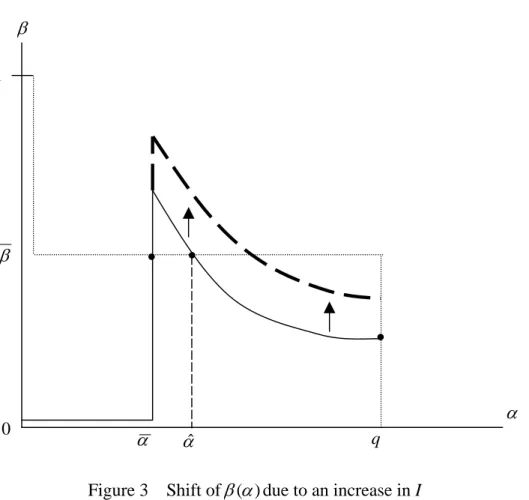
[Insert Figures 2 and 3 about here]
Suppose that ( ; ) is not the equilibrium outcome at the status quo. If we pour more resources into the IRS, the IRS’s best-response curve will be shifted upward as shown in Figure 3. If we keep on pouring, it is clear that( ; ), similar to that shown in Figure 1c, will eventually result as the unique equilibrium outcome. In contrast to outcomes ^;
and(q;Ic)where the marginal tax revenue is greater than the marginal cost of collection (i.e.
R( ^) > c and R(q) > c), the IRS equates the marginal tax revenue to the marginal cost of collection under the outcome ( ; ) (i.e. R( ) = c). Since outcome ( ; ) yields the least cost per dollar of tax collection, we obtain
Corollary 1 The size of the budget allocated to the IRS should be expanded as long as an additional dollar allocated could return more than an additional dollar of tax revenue.
A tax farmer, who is interested only in pro…t maximization, will expand the size of her audit resources if an additional dollar of audit input could return more than an additional dollar of tax revenue. Corollary 1 requires that the Congress support the “IRS as tax farmer.”16 This policy prescription contrasts with Slemrod and Yitzhaki’s (1987) …nding that the marginal tax revenue exceeds the marginal cost of collection at the optimum and,
consequently, the “IRS as tax farmer”would lead to a socially excessive amount of resources devoted to tax collection. Put di¤erently, the Congress should provide a smaller budget than the IRS would wish according to Slemrod and Yitzhaki, whereas the Congress should provide the budget that the IRS would wish according to our model.
To ensure that( ; ) is the unique equilibrium outcome, I > c must hold (see Table 1). Since the size of the population who report nothing equals ( + 1 q) in equilibrium and since the IRS incurs a costcfor each person it veri…es, the meaning of the inequality I > c
is clear: even if = q (i.e. all taxpayers evade) so that + 1 q = 1, the size of the budget allocated should still enable the IRS to support an audit probability higher than (i.e. I
c( +1 q) =
I
c > ). The intuition behind this result is simple. Note that the taxpayers
will comply if they expect > . When I > c, it is feasible for the IRS to support an audit probability higher than at all possible realized ’s: This feasibility completely eliminates the taxpayers’self-ful…lling expectations that a widespread and rampant evasion may “congest” the IRS’s tax administration to such an extent that it becomes impossible for the IRS to maintain > at some high ’s. By contrast, the taxpayers’self-ful…lling expectations could support the realization of = ^ or =q if I c.17
(Toma and Toma, 1992). However, one might worry about whether taxpayers’private information should be possessed by private agents. Through H.R. 4520, American Jobs Creation Act of 2004, the Congress gives the IRS the authority to use private collection agencies to collect IRS debt and pay them a bounty of up to 25 percent of the money they collect. This statute is strongly opposed by National Treasury Employees Union. One reason raised for the opposition is: “the IRS does not have the technology in place to ensure that taxpayer information is kept secure and con…dential when it is handed over to the private collection agencies.” (Kelley, 2005)
17At =q, the maximal probability of audit that the IRS can support equals I c. If
I
c is greater than ,
the equilibrium( ; )can be ensured. If I
c is not greater than , the equilibrium( ; )cannot be ensured.
We focus on lifting Ic above by increasingI. There is another side of the same coin: lifting Ic above by reducingc. We comment on this alternative possibility at the end of the paper.
4.2
Intuition
As noted before, Slemrod and Yitzhaki (1987) and others, including Usher (1986), Kaplow (1990), Mayshar (1991) and Sanchez and Sobel (1993), all conclude that the size of the budget allocated to the IRS should fall short of equating the marginal revenue with the marginal cost of tax collection, whereas we conclude that it should equate the marginal revenue with the marginal cost of tax collection. Is there any intuition behind the di¤erence? In this subsection we provide one.
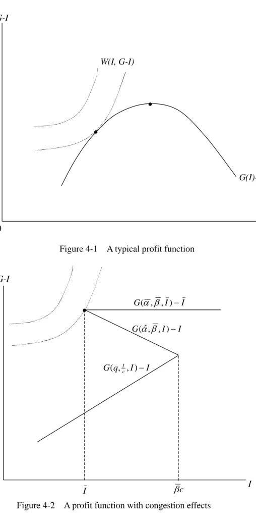
Mayshar (1991) views the maximal tax revenue collected as a function of the IRS’s en-forcement budget and other variables such as the tax base and tax structure. He calls this function a “tax technology.” Like the standard production function of the …rm, the tax technology is a “black box” and its details are left unspeci…ed. Because of the “black box” nature, Mayshar’s tax technology can be interpreted to accommodate a variety of models, including Slemrod and and Yitzhaki’s commitment model and our non-commitment model. Speci…cally, in terms of our notation, we can simply writeG = G(I), where G(:) represents the tax technology. The net tax revenue or “pro…t” is then represented byG(I) I.
What doesG(I) I look like? Mayshar (1991) argues that it takes the shape of a La¤er curve as shown in Figure 4-1.18 This shape seems to be typical for a pro…t function. Let us impose the set of indi¤erence curves of a social welfare functionW(I; G I)with @W
@I <0
and @(@WG I) >0on the “La¤er curve.” It is easy to see from Figure 4-1 that the optimal level ofI is always lower than the level selected by the “pro…t-maximizing” IRS.
[Insert Figure 4 about here]
Figure 4-2 shows the shape of G(I) I in our model.19 The “pro…t”G(I) I increases
withI continuously until the level of I reaches I. FromI on,G(I) I takes a zigzag shape
18See Figure 1 in Mayshar (1991).
rather than the standard shape of a La¤er curve and, in particular, the value of G(I) I
may jump discontinuously asI varies. The reason for the discontinuous jump in “pro…t” is obviously attributable to the existence of multiple equilibria, which are in turn attributable to the mitigation (if = ^ rather than = q) or even elimination (if = rather than = q) of the congestion e¤ect.20 This mitigation or elimination of the congestion
e¤ect becomes feasible only if the size of the budget allocated to the IRS is large enough to satisfyI I. Let us impose the same set of indi¤ernce curves of the social welfare function
W(I; G I) on the “zigzag curve.” It is easy to see from Figure 4-2 that the equilibrium outcome ( ; ) = ( ; ) with I = I is the optimal solution. As we have explained in Figure 3, this optimal solution can be implemented by supporting the “IRS as tax farmer” and expanding the size of the budget allocated to the IRS as long as the marginal revenue is greater than the marginal cost of tax collection.
5
Extension
The model presented so far may well represent a particular audit class only, where the audit class is sorted on the basis of some observable taxpayer characteristics such as zip code, reported income level/source, occupation or age. GRW and Erard and Feinstein (1994), among others, interpret their audit rules within, not across, audit classes. The same kind of interpretation is equally applicable to our previous setting. In this section we consider an economy-wide model in which there are two or more audit classes.
Consider an economy in which there are n 2 audit classes. Except for the audit cost, each audit class has identical structures and parameters as before. Without loss of generality, let0< c1 < c2 < < cn. We could consider a more general setting in which incomes earned
20Remember that the congestion e¤ect is captured in our model by the downward-sloping part of the IRS’s
vary across di¤erent audit classes. Speci…cally, leti and j denote two di¤erent audit classes, and Ti < Tj and Fi < Fj if yi < yj (i.e. the higher the income earned in an audit class, the
more the tax that needs to be paid and the larger the …ne that needs to be imposed if evasion is detected). However, Proposition 1 reveals that what matters to our model is the relative rather than absolute relation betweenT +F and c(i.e. R(q) = q(T +F) relative toc). In view of this, we letyi =yj and focus on the case whereci 6=cj for simplicity.21
IfR(q) ci, it is not pro…table for the IRS to audit classi. We then have the same result
as Proposition 1 (i)-(ii), that is, i =q and variations in I exert no impact on i. Similar to Proposition 2, we con…ne our analysis to the cases whereR(q)> ci.
Now suppose that R(q)> cn. De…ne i as the amount of i such that the IRS is merely
indi¤erent between auditing and not auditing class i (i.e. R( i) = ci). Let Ii 0 be the
IRS’s budget allocation intended for auditing classiwithPni=1Ii =I. We have the following
extension of Proposition 2.22
Proposition 3 Of all possible equilibrium outcomes, f i; gni=1 yields the least cost per 21Reinganum and Wilde (1986) extend the GRW model (without habitual compliers) to the situation where
a taxpayer’s income can take any value in some range. They focus on the fully separating equilibrium. As Erard and Feinstein (1994) point out, an unrealistic feature of this separating solution is that the IRS knows the true income of each taxpayer prior to performing any tax audit, even though in actual practice this is often not the case. Erard and Feinstein (1994) incorporate habitual compliers into the Reinganum-Wilde model, showing that the incorporation has important impacts on the equilibrium solution and, in particular, that it resolves the unrealistic feature mentioned above. The cost paid is that the resulting equilibrium is characterized by a highly nonlinear second-order di¤erential equation, and Erard and Feinstein have to rely extensively on simulations to study the solution of their model. It should be noted that Erard and Feinstein (1994) do take into account the IRS’s budget constraint. However, there are no multiple equilibria associated with the congestion e¤ect in their model. Like GRW0, Erard and Feinstein (1994) do not address the e¢ ciency issue.
22The budget allocation fI
1; I2; :::; Ing that supports the outcome ( i; ) (i = 1;2; :::; n) is not unique.
dollar of tax collection.
When there is only one audit class, I > c must hold in order to ensure the least cost equilibrium outcome ( ; ) (see Table 1). What is the corresponding condition when there are two or more audit classes? The following proposition provides the answer.
Proposition 4 To support f i; gni=1 as the unique equilibrium outcome of the game, I >
[cn+ Pn 1 i=1( ~i+ 1 q)ci] must hold, where f~igni=11 satisfy R( ~1) c1 = R( ~2) c2 = = R( ~n 1) cn 1 = R(q) cn : (5)
Remark 3 Melumad and Mookherjee (1989) argue that it is di¢ cult for a government to commit to the allocation of aggregate audit costs or aggregate revenues collected, but it is reasonable to assume that the government can make commitments based on these aggregate variables since they are publicly available as part of the process of budgetary appropriations and reviews of tax-collection agencies. Our setting is consistent with this argument since the Congress can controlI, but not Ii.
Remark 4 Erard and Ho (2004) use information from two data …les of the IRS’s Taxpayer Compliance Measurement Program for the tax year 1988 (one for those who …le tax returns and the other for those who do not …le tax returns) plus supplementary information on tip earners and informal suppliers to study the tax compliance behavior of 34 distinct occupational groups in the U.S. economy. They …nd that the share of tax liability that goes unpaid is 14.9% on average for all occupations as a whole, but that it varies substantially across di¤erent occu-pations, ranging from 51.1% (vehicle sales), 49.8% (tip earners), 44.1% (informal suppliers), 16.0% (mechanics and repairers), and 7.0% (doctors and dentists), to 5.4% (accountants,
au-ditors and tax preparers). Since R( i)
ci =
R( j)
cj for i6=j,
@R
@ >0and 0< c1 < c2 < < cn,
audit classes are sorted on the basis of occupations, this result is consistent with Erard and Ho’s …nding with regard to the U.S. tax compliance continuum across occupations.
The intuition underlying Proposition 4 is as follows. First, it is not possible to have
i = j = q for i 6= j, since this would lead to R(q)
ci 6=
R(q)
cj (the IRS can then improve her
pro…t by re-allocating the budget between audit classes i and j). Thus, in any equilibrium there is at most one audit class such that all taxpayers cheat. Furthermore, this audit class must be thenth class because 1 < 2 < ::: < n qand the corresponding equilibrium must satisfy equation (5). The inequality condition stated in Proposition 4 essentially requires that the total budget allocated to the IRS be large enough for her to kill o¤ this equilibrium. In Table 1,( ; )is the only equilibrium outcome that will survive once the budget size is large enough to eradicate the most “congestive” equilibrium evasion (i.e. = q). Analogously, in our extended model, f i; gni=1 is the only equilibrium outcome that will survive once
the budget size is large enough to eradicate the most “congestive” equilibrium evasion (i.e.
i = ~i fori= 1;2; :::; n 1 and n =q).
6
Conclusion
We conclude our paper with four remarks. First, suppose that the audit classes in Section 5 are sorted on the basis of occupations. We can then extend our model to incorporate the taxpayers’ occupational choice before the Congress’s budget allocation.23 As long as
the size of the budget allocated is large enough to support the least cost equilibrium as the unique outcome, the IRS’s auditing activities will not distort the taxpayers’ occupational choice. This is because the equality iu(y T F) + 1 i u(y) = u(y T) holds for
23One can reverse the order of the choices: adding the taxpayers’occupational choice after the Congress’s
budget allocation. However, it seems that the occupational choice is a longer decision than the yearly budget allocation.
all i = 1;2; :::; n at the least cost equilibrium. That is, all taxpayers in all occupations are indi¤erent between evasion and compliance. This equality also indicates that horizontal equity in the ex ante sense will be obeyed. Other equilibria need not possess such desirable properties. For example, consider the equilibrium that satis…es equation (5). The outcome resulting from this equilibrium not only distorts the taxpayers’occupational choice but also violates horizontal equity. This is because the taxpayers in thenth audit class enjoy a higher expected utility than the taxpayers in other audit classes.
Second, Kau and Rubin (1981, p. 262) hypothesize that “there have been changes in pro-duction technologies which have directly led to an increase in the proportion of income which is subject to taxation.” These changes are attributable to factors such as fewer self-employed individuals, improved record keeping due to increased incorporation, and the substitution of market production for home production. All of these changes presumably lower the IRS’s cost of tax audits. North (1985, p. 392) puts forth a similar hypothesis: “The supply of government was made possible by new technology which, coupled with the consequences of growing market specialization, lowered the costs of government monitoring of income and wealth and increased the e¢ ciency of government taxation.” Kau and Rubin (1981) …nd em-pirical support for their hypothesis, and Ferris and West (1996) provide additional emem-pirical support. In terms of our model, a lower cost of tax audit has three main e¤ects: (i) it turns some taxpayers from being “hard-to-tax” into “not-so-hard-to-tax” (i.e. from R(q) c to
R(q)> c in Proposition 1), (ii) it lowers the threshold evasion that makes the IRS indi¤erent between auditing and not auditing (i.e. a lower de…ned in equation (1)), and (iii) it raises the probability of audit that the IRS can support under a budget constraint (i.e. a higher
I
c( +1 q)). These e¤ects are obviously important and should not be ignored. Nevertheless, as
far as the yearly budget appropriation is concerned, it does not seem unreasonable to view the audit costcas a parameter, which is beyond the control of both the IRS and the Congress.24
Third, according to our model, the IRS will let go of “hard-to-tax”taxpayers. Increasing the size of the budget allocated to the IRS can do little about it. This result is attributed to the fact that there is a negative return on money invested in “hard-to-tax”taxpayers for the IRS. Wertz (1979) observes that the IRS is often expected by the Congress to “show a pro…t” on her enforcement activities. This could aggravate the “hard-to-tax” problem. Fixing the “hard-to-tax” is a thorny task and alternative strategies such as exempting these taxpayers or simply ignoring them have been proposed. We refer those who are interested in the issue to Alm et al (2004).
Fourth, we provide a case for the policy prescription that the size of the budget allocated to the IRS should be expanded as long as an additional dollar allocated could return more than an additional dollar of tax revenue (Corollary 1). Of course, like …ndings in other theoretical models, this result is built upon several assumptions which abstract a parsimonious model from the complicated real world. An assumption of the GRW model, on which our model is based, is that individual incomes take one of only two values (either high or low). This assumption may be restrictive in that it reduces the taxpayer problem to a simple comply/do not comply decision.25 Other assumptions such as that true income will be discovered once a tax audit is performed, and that taxpayers su¤er no additional cost during the auditing process may be problematic as well. It is arguable that the tax code itself is imperfect and that tax auditors are not uniform in interpreting the tax code. As a result, the so-called “true income” may never be known. “Mention the IRS, most people think of the dreaded tax audit.” This vivid description of the IRS’s tax audit by Slemrod and Bakija
program. The implementation of this program is expected to reduce the IRS’s audit cost in the future; see IRS Oversight Board (2006).
25Two points are worth mentioning, however. First, as noted in footnote 5, there are two possible
interpre-tations for non-compliance in our model: underreporting and non-…ling. Whether or not to …le tax returns is by nature a binary comply/do not comply decision. Second, we have extended the GRW model to multiple audit classes in Section 5.
(2004, p. 180) suggests that the auditing process itself may be highly costly to taxpayers. Note also that …ling tax returns per se is assumed costless for individuals in our model. This seems inconsistent with the substantial e¤orts exerted by the IRS to provide the so-called “taxpayer service.” Indeed, according to Professor Slemrod’s (2005) testimony to the President’s Advisory Panel on Federal Tax Reform, complying with the tax code per se costs individual taxpayers approximately $85 billion a year. Despite these and other possible limitations of our model, we believe we have brought a fresh perspective to the important issue of how much to fund the IRS. Kaplow (1996, p. 144) wrote:
“In the academic literature, it is well understood (although not always re-membered or emphasized) that the proper cost-bene…t analysis does not simply compare the enforcement cost to the revenue raised.”
This claim may need to be quali…ed based on the thrust of this paper.
7
Appendix
Proposition 1.
Proof. (i) If R(q) 2 [0; c), the IRS’s incremental expected revenue from a tax audit will always be less than her audit cost spent, regardless of what is. Hence, the IRS never audits, that is = 0. Since the IRS never audits, the taxpayer has no incentive to report yand, as a result, =q.
(ii) Suppose thatR(q) =c. If < q, the IRS has no incentive to audit since R( )< c
for all < q. This implies that ( ) = 0. However, with ( ) = 0 < , every taxpayer would strictly prefer cheating, that is, = q, which yields a contradiction. This leaves us only the case of = q. Given R(q) = c, the IRS is indi¤erent between auditing and not auditing, that is, (q) 2 [0;minfIc;1g]. However, for all taxpayers to choose cheating, we require that (q) . Hence, we obtain 2[0;minfIc; g].
(iii) Suppose that R(q) > c. Since R(0) = 0 and @R
@ > 0, we have a unique 2 (0; q)
such thatR( ) =c. This unique is the de…ned in (1). Note that the sign of R( ) cis the same as the sign of . The IRS’s best audit response to with the budget constraint is thus given by ( ) = 8 > > > < > > > : minfc( +1I q);1g if > 2[0;minf I c( +1 q);1g] if = 0 if <
where > implies R( ) > c so that the IRS will either exhaust all her budget with
( ) = c( +1I q) or reach ( ) = 1; < implies R( ) < c so that it is not pro…table for the IRS to carry out any tax audit with ( ) = 0; and = implies R( ) = cso that the IRS is indi¤erent between auditing and not auditing.
A taxpayer’s best response will depend on his expectation concerning . If he expects
> , he will reporty. If < , he will report nothing. If = , he is indi¤erent.
Suppose < , then ( ) = 0, which implies that every taxpayer strictly prefers cheating, that is, =q > , a contradiction.
Suppose = ; then ( = ) 2 [0;minf I
c( +1 q);1g]. Since 2 (0; q), it is required
that a taxpayer be indi¤erent between reportingy and reporting nothing. Because is the audit probability that makes the taxpayer indi¤erent between reporting and not reporting, the only equilibrium in this case is ( = ) = . Note that ( = )2[0;minf I
c( +1 q);1g].
Therefore, c( +1I q) or, equivalently,I c( + 1 q).
Suppose 2 ( ; q), then ( ) = minfc( +1I q);1g. To support 2 ( ; q), which implies that a taxpayer is indi¤erent between reportingyand not reporting, we need ( ) =
I
c( +1 q) = ; that is, = ^ and = . Since ^ 2 ( ; q), we have I = c( ^ + 1 q) 2
( ( + 1 q)c; c).
Suppose =q, then ( ) = minfc(q+1I q);1g= minfIc;1g. To support =q, which implies that a taxpayer prefers cheating, it is required that ( =q) = Ic . Hence, we
obtainI c .
To sum up, ( ; ) = ( ; ) could result if I c( + 1 q); ( ; ) = ^; could result if ( + 1 q)c < I < c; and ( ; ) = (q;Ic) could result ifI c.
Proposition 2.
Proof. First, consider the comparison between ; and( ^; )when ^ 6= . We know that
^ > and thatT > (T +F) (Result 1). Invoking these two results, it is straightforward to see from Table 1 that G ^; ; I < G ; ; I . Since I < I if ^ 6= , we also see from Table 1 thatS ^; ; I > S ; ; I . Putting these together yields ; ; I < ^; ; I . That is, outcome( ^; ) always yields a higher cost per dollar of tax collection than outcome
( ; ) if ^6= .
Next, consider the comparison between ; and q;Ic . We will …rst show that (q;Ic; I)
is strictly decreasing in I. Since ; ; I is a constant, all we are left to show is that
(q;Ic; I) remains higher than ( ; ; I) at I = c, the maximal size of the budget beyond which the equilibrium with outcome(q;Ic) will no longer exist (see Proposition 1 (iii)).
From (3) and (4), we see thatC is strictly increasing and concave in (Result 2). There-fore, for any 2 (0;1) and x > 0, we have C(x) + (1 )C(0) < C( x+ (1 ) 0). This leads to C(x) < C( x), since C(0) = 0 by the de…nition of C in equation (2). Now, for anyI < I0, choosing = I
I0 and x= I0 c gives I I0C I0 c < C I
c . Utilizing this result, we
have (q;I c; I) = qC Ic +I I cq(T +F) > q I I0C I0 c +I I cq(T +F) = qC I0 c +I0 I0 cq(T +F) = (q; I 0 c; I 0):
This proves that (q;Ic; I) is strictly decreasing in I. AtI = c, we have (q;Ic) = ^; (Remark 1). Thus,
G q;I
c; I =G( ^; ; I) = (q ^)T + ^ (T +F) <(q )T + (T +F) =G ; ; I :
At I = c, we also have S q;I c; I =qC( I c) +I =qC + c > qC + ( + 1 q)c =S ; ; I :
Since G q;Ic; I < G ; ; I and S q;Ic; I > S ; ; I at I = c, we obtain ( ; ; I)< q;Ic; I at I = c.
Thus, for all I 2[I;1) (where the equilibrium( ; ) may result) andI0 2[0; c] (where
the equilibrium q;Ic may result),
; ; I = ; ; I < q; I
c; I = c q;
I0
c; I
0
where the last inequality has utilized the property that is decreasing inI. This means that
( ; ) gives a lower cost per dollar of tax collection than q;I c . Proposition 3.
Proof. First, if there exists anisuch that i < i, then from the de…nition of i and because @R
@ >0, we know thatR( i)< ci and hence the IRS will choose i = 0. This implies that
the taxpayers will all cheat, i.e., i =q, a contradiction. Hence, we must have i i for all
i. Next, we can check that if f( i; i)gni=1 is an equilibrium outcome, then either i 2[ i; q)
and i = , or i = q and i = Ii
ci . Putting these together, we conclude that the
resulting equilibrium outcomes in an audit class qualitatively follow that of Proposition 1 (iii). Finally, viewing the role of Ii intended for audit class i as that ofI in the case of one
audit class, the rest of the proof then follows the same logic as the proof of Proposition 2.
Proposition 4.
Proof. First, note that R( i) = i 1i q(T +F) is strictly increasing and continuous in i.
Since R( i)
ci = 1and
R(q)
ci >
R(q)
cn >1 (i= 1;2; :::; n 1), from the intermediate value theorem
Step 1. Suppose that I [cn+Pin=11( ~i + 1 q)ci] . It is straightforward to check
that there exists an equilibrium outcome f( i; i)gn
i=1 such that ( i; i) = ( ~i; ) for i =
1; : : : ; n 1 and ( n; n) = q;In
c , where In = I
Pn 1
i=1 ( ~i+ 1 q)ci . First, given i = ~i (i= 1;2; :::; n 1)and n=q, we see from equation (5) that the incremental revenue
per dollar of tax audit is the same across all classes. This implies that the IRS cannot improve her pro…t by re-allocating the budget between di¤erent audit classes and changing
i. Next, given i = i (1;2; :::; n 1)and n = cInn, we see that i = ~i (i= 1;2; :::; n 1)
is consistent with i = i = (i = 1;2; :::; n 1) and that n = q is consistent with n = Icnn (Since I [cn+
Pn 1
i=1( ~i + 1 q)ci] by assumption, we obtain In cn from
In =I Pin=11( ~i+ 1 q)ci ).
Step 2. Suppose thatI >[cn+Pni=11( ~i+ 1 q)ci] . We show below thatf( i; i)gni=1 =
f i; gni=1, that is,f i; gni=1 is the unique equilibrium outcome of the game.
First, R( i)
ci must equal a constant for all i = 1;2; : : : ; n. Suppose not, and let i0 be the
audit class which has the highest incremental revenue per dollar of tax audit (i.e. R( i0)
ci0
>
R( i)
ci for i 6= i0). This implies that the IRS will audit the class i0 with the …rst priority.
Since I ( i0+1 q)ci0 > I ci0 > ( I ci0 I cn > + Pn 1 i=1( ~i+ 1 q) ci cn ), we have i0 > , which leads to i0 = 0. However, note that R i
0 = 0 = 0and
R( i)
ci 0 for alli= 1; : : : ; n, which
yields a contradiction with R( i0)
ci0 >
R( i)
ci for i6=i0.
Secondly, R( i)
ci = 1 must hold for all i = 1; : : : ; n. Suppose not. If
R( i)
ci < 1, the
IRS would have no incentive to audit and so i = 0. This leads to i = q for all i and
R(q)
ci >
R(q)
cn > 1, a contradiction. If
R( i)
ci > 1, the pro…t-maxmizing IRS will exhaust the
budget intended for each audit class. Sinceci is strictly increasing in i, i must be strictly
increasing iniin order to have a constant R( i)
ci for all i. Because of 1 < 2 < ::: < n q,
the highestf igni=1 that generates the same incremental revenue per dollar of tax audit is that
i = ~i for i= 1; : : : ; n 1 and n =q. This implies that i ~i < q for i = 1; : : : ; n 1,
(i= 1;2; :::; n 1) together yields In=I n 1 X i=1 ( i + 1 q) ici > I n 1 X i=1 ( ~i+ 1 q) ci > cn
where the …rst equality has utilized the result that the IRS will exhaust the budget intended for each class and the last inequality comes from our premise. Therefore, we have n= In
cn > ,
which leads to n = 0, a contradiction. Since R( i)
ci = 1for alli= 1; : : : ; n, we have i = i(i= 1; : : : ; n). To support i 2(0; q)
such that the taxpayers are indi¤erent between auditing and not auditing, i = must be true.
References
[1] Allingham, M.G, Sandmo, A., 1972. Income tax evasion: a theoretical analysis. Journal of Public Economics 1, 323-338.
[2] Alm, J., Martinez-Vazquez, J., Wallace, S. (Eds.), 2004. Taxing the Hard-to-Tax: Lessons from Theory and Practice. Elsevier Science, Amsterdam.
[3] Andreoni, J., Erard, B., Feinstein, J. 1998. Tax compliance. Journal of Economic Liter-ature 36, 818-860.
[4] Bird, R.M., Casanegra de Jantscher, M., 1992. The reform of tax administration. In: R.M. Bird, M. Casanegra de Jantscher (Eds.), Improving Tax Administration in Developing Countries. IMF, Washington, DC.
[5] Chu, C.Y., 1990. Plea bargaining with the IRS. Journal of Public Economics 41, 319-333. [6] Cowell, F.A., 1990. Tax sheltering and the cost of evasion. Oxford Economic Papers 42,
[7] Cowell, F.A., 2004. Sticks and carrots in enforcement. In: H.J. Aaron, J. Slemrod (Eds.), The Crisis in Tax Administration. Brookings Institution Press, Washington, DC.
[8] Cowell, F.A., Gordon, J.P.F., 1995. Auditing with ghosts. In: G. Fiorentini, S. Peltzman (Eds.), The Economics of Organized Crime. Cambridge University Press, Cambridge. [9] Erard, B., Feinstein, J.S., 1994. Honesty and evasion in the tax compliance game. RAND
Journal of Economics 25, 1-19.
[10] Erard, B., Ho, C.-C., 2001. Searching for ghosts: who are the non…lers and how much tax do they owe? Journal of Public Economics 8, 25-50.
[11] Erard, B., Ho, C.-C., Mapping the US tax compliance continuum. In: J. Alm, J. Martinez-Vazquez, S. Wallace (Eds.), Taxing the Hard-to-Tax: Lessons from Theory and Practice. Elsevier Science, Amsterdam.
[12] Ferris, J.S., West, E.G., 1996. Testing theories of real government size –US experience, 1959-89. Southern Economic Journal 62, 537-553.
[13] Graetz, M.J., Reinganum, J.F., Wilde, L.L., 1984. A model of tax compliance with budget-constrained auditors. Social Science Working Paper no. 506, California Institute of Technology.
[14] Graetz, M.J., Reinganum, J.F., Wilde, L.L., 1986. The tax compliance game: toward an interactive theory of tax enforcement. Journal of Law, Economics, and Organization 2, 1-32.
[15] Gul, F., Sonnenschein, H., Wilson, R., 1986. Foundations of dynamic monopoly and the Coase conjecture. Journal of Economic Theory 39, 155-190.
[16] IRS, 1996. Federal Tax Compliance Research: Individual Income Tax Gap Estimates for 1985, 1988, and 1992. IRS Publication 1415 (Revised 4/96), Washington DC.
[17] IRS Oversight Board, 2006. FY2007 IRS Budget Recommendations, Special Report. IRS Oversight Board, Washington, DC.
[18] Kalai, E., 2004. Large robust games. Econometrica 72, 1631-1665.
[19] Kaplow, L., 1990. Optimal taxation with costly enforcement and evasion. Journal of Public Economics 43, 221-236.
[20] Kaplow, L., 1996. How tax complexity and enforcement a¤ect the equity and e¢ ciency of the income tax. National Tax Journal 49, 135-150.
[21] Kau, J.B., Rubin, P.H., 1981. The size of the government. Public Choice 37, 261-274. [22] Kelley, C.M., 2005. Statement of Collen M. Kelley, National Treasury Employees Union.
Hearing Archives, Committee on Ways and Means.
[23] Los Angeles Times, 1987. Last-minute tax rush to delay refunds. April 14.
[24] Macho-Stadler, I., Perez-Castrillo, D.J., 1997. Optimal auditing with heterogeneous in-come sources. International Economic Review 38, 951-968.
[25] Mayshar, J., 1991. Taxation with costly administration. Scandinavian Journal of Eco-nomics 93, 75-88.
[26] Melumad, N.D., Mookherjee, D., 1989. Delegation as commitment: the case of income tax audits. RAND Journal of Economics 20, 139-163.
[27] North, D.C., 1985. The growth of government in the United States: an economic histo-rian’s perspective. Journal of Public Economics 28, 383-399.
[28] Reinganum, J.F., Wilde, L.L., 1985. Income tax compliance in a principal agent frame-work. Journal of Public Economics 26, 1-18.
[29] Reinganum, J.F., Wilde, L.L., 1986. Equilibrium veri…cation and reporting policies in a model of tax compliance. International Economic Review 27, 739-760.
[30] Reinganum, J.F., Wilde, L.L., 1988. A note on enforcement uncertainty and taxpayer compliance. Quarterly Journal of Economics 103, 793-798.
[31] Sanchez, I., Sobel, J., 1993. Hierarchical design and enforcement of income tax policies. Journal of Public Economics 50, 345-369.
[32] Sandmo, A., 2005. The theory of tax evasion: a retrospective view. National Tax Journal 58, 643-663.
[33] Slemrod, J., 2005. Statement of Professor Joel Slemrod, University of Michigan Ross School of Business, before the President’s Advisory Panel on Federal Tax Reform. March 3.
[34] Slemrod, J., Bakija, J. 2004. Taxing Ourselves: A Citizen’s Guide to the Debate over Taxes, Third Edition. MIT Press, Cambridge.
[35] Slemrod, J., Yitzhaki, S., 1987. The optimal size of a tax collection agency. Scandinavian Journal of Economics 89, 183-192.
[36] Slemrod, J., Yitzhaki, S., 2002. Tax avoidance, evasion, and administration. In: A.J. Auerbach, M, Feldstein (Eds.), Handbook of Public Economics, Vol. 3. North-Holland, Amsterdam.
[37] Thuronyi, V. 2004. Presumptive taxation of the hard-to-tax. In: J. Alm, J. Martinez-Vazquez, S. Wallace (Eds.), Taxing the Hard-to-Tax: Lessons from Theory and Practice. Elsevier Science, Amsterdam.
[38] Toma, E.-F., Toma, M., 1992. Tax collection with agency costs: private contracting or government bureaucrats? Economica 59, 107-120.