University of Colorado, Boulder
CU Scholar
Electrical, Computer & Energy Engineering
Graduate Theses & Dissertations
Electrical, Computer & Energy Engineering
Spring 1-1-2011
Dynamic Trace Analysis with Zero-Suppressed
BDDs
Graham David Price
University of Colorado at Boulder, [email protected]
Follow this and additional works at:
http://scholar.colorado.edu/ecen_gradetds
Part of the
Computer Sciences Commons
, and the
Engineering Commons
This Dissertation is brought to you for free and open access by Electrical, Computer & Energy Engineering at CU Scholar. It has been accepted for inclusion in Electrical, Computer & Energy Engineering Graduate Theses & Dissertations by an authorized administrator of CU Scholar. For more information, please [email protected].
Recommended Citation
Price, Graham David, "Dynamic Trace Analysis with Zero-Suppressed BDDs" (2011).Electrical, Computer & Energy Engineering Graduate Theses & Dissertations.Paper 27.
B.S. University of Evansville, 2002
M.S. University of Colorado at Boulder, 2006
A thesis submitted to the
Faculty of the Graduate School of the
University of Colorado in partial fulfillment
of the requirements for the degree of
Doctor of Philosophy
Department of Electrical, Computer, and Energy Engineering
Dynamic Trace Analysis with Zero-Suppressed BDDs written by Graham David Price
has been approved for the Department of Electrical, Computer, and Energy Engineering
Manish Vachharajani, Ph.D. (Chair)
Fabio Somenzi, Ph.D.
Bor-Yuh Evan Chang, Ph.D.
Jeremy G. Siek, Ph.D.
Tipp Moseley, Ph.D. (Outside Member)
Date
The final copy of this thesis has been examined by the signatories, and we find that both the content and the form meet acceptable presentation standards of scholarly work in the above mentioned discipline.
Dynamic Trace Analysis with Zero-Suppressed BDDs
Thesis directed by Professor Manish Vachharajani, Ph.D. (Chair)
Instruction level parallelism (ILP) limitations have forced processor manufacturers to develop
multi-core platforms with the expectation that programs will be able to exploit thread level parallelism (TLP).
Multi-core programming shifts the burden of locating additional performance away from computer hardware to the
software developers, who often attempt high-level redesigns focused on exposing thread level parallelism, as
well as explore aggressive optimizations for sequential codes.
Precise dynamic analysis can provide useful guidance for program optimization efforts, including
efforts to find and extract thread level parallelism. Unfortunately, finding regions of code amenable to further
optimization efforts requires analyzing traces that can quickly grow in size. Analysis of large dynamic traces
(e.g. one billion instructions or more) is often impractical for commodity hardware.
An ideal representation for dynamic trace data would provide compression. However, decompressing
large software traces, even if decompressed data is never permanently stored, would make many analysis
impractical. A better solution would allow analysis of the compressed data, without a costly decompression
step. Prior works have developed trace compressors that generate an analyzable representation, but often
limit the precision or scope of analyses.
Zero-suppressed binary decision diagram (ZDDs) exhibit many of the desired properties of an ideal
trace representation. This thesis shows: (1) dynamic trace data may be represented by zero-suppressed
binary decision diagrams (ZDDs); (2) ZDDs allow many analyses to scale; (3) encoding traces as ZDDs can
be performed in a reasonable amount of time; and, (4) ZDD-based analyses, such as irrelevant instruction
detection and potential coarse-grained thread level parallelism extraction, can reveal a number of performance
Dedication
Acknowledgements
I would like to thank my research adviser Dr. Manish Vachharajani who provided the perfect blend of
brilliant insight, inspiration, and constructive feedback. Without his talents and aid, I simply would not have
competed this thesis, nor would I have the desire to continue to explore.
The help I received at the University of Colorado was necessary for the completion of this degree, but
Contents
Chapter
1 Introduction 1
1.1 Dynamic Trace Compression . . . 1
1.2 Dynamic Trace Analysis at Scale . . . 3
1.3 Opportunities for Optimization . . . 3
1.4 Contributions . . . 5
1.5 Hypothesis . . . 7
2 Parallel Computation Background 8 2.1 Automatic Parallelization Techniques . . . 8
2.1.1 Automatic Parallelization by Static Analysis . . . 9
2.1.2 Automatic Parallelization by Dynamic Analysis . . . 12
2.2 Parallelization with Tools . . . 15
3 Related Works 18 3.1 Dynamic Trace Compression . . . 18
3.1.1 Abstraction and Elimination . . . 18
3.1.2 SEQUITUR Compression . . . 19
3.1.3 Sequential Compressed Traces . . . 20
3.2 Reduced Ordered Binary Decision Diagrams . . . 20
3.5 Dynamic Trace Analysis . . . 24
3.6 DINxRDY Visualizations . . . 24
3.6.1 Dynamic Program Slicing . . . 27
3.6.2 Hot Code Analysis . . . 27
3.7 Parallelism in Computing . . . 27
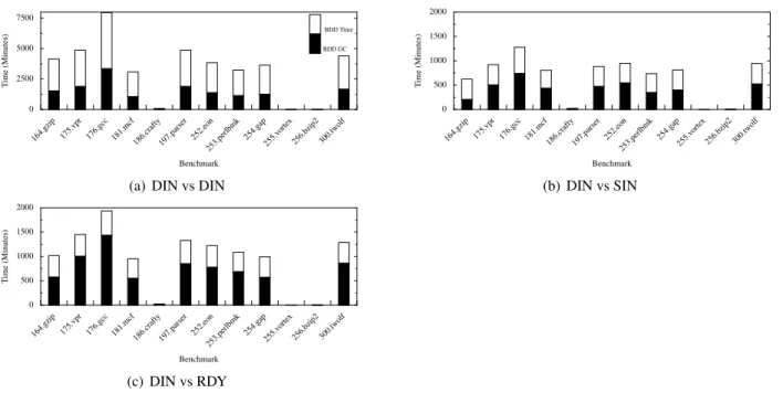
4 Dynamic Trace Analysis at Scale 29 4.1 BDD Compression Time . . . 29
4.1.1 Traces as Boolean Functions . . . 29
4.1.2 Boolean Functions as BDDs . . . 30
4.1.3 BDD Unique Tables . . . 31
4.1.4 Garbage Collection and Compression Time . . . 32
4.2 ZDD Compressed Traces . . . 37
4.2.1 BDDs vs. ZDDs . . . 37
4.2.2 Traces as ZDDs . . . 37
4.2.3 ZDD Variable Order, Visualization, and Analysis . . . 41
4.2.4 ZDD Compression Time . . . 41
4.3 ZDD Dependence Visualization . . . 45
4.3.1 DINxRDY Visualization . . . 45
4.3.2 Extended Visualization Algorithm . . . 49
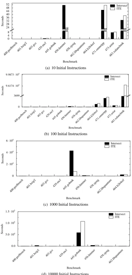
5 ZDD-based Dynamic Trace Slicing and Chopping 53 5.1 ZDD Slice Performance . . . 54
5.1.1 Experimental Setup . . . 56
6 Irrelevant Component Elimination 58 6.1 Visualization Filtering . . . 65
6.1.1 Experimental Setup . . . 65
6.1.2 Ready Filter . . . 66
6.1.3 Irrelevant Instruction Filter . . . 70
6.1.4 Dead-Hot Filter . . . 70
7 Coarse-Grained Thread Level Parallelism 74 7.1 TLP Visualization with ParaMeter . . . 75
7.2 Region Selection . . . 75
7.3 ZDD Slicing . . . 80
7.4 ZDD Chopping . . . 83
7.5 Potential Coarse-Grained Thread Level Parallelism in SPEC INT 2006 . . . 85
7.5.1 Fine-Grained Harmony . . . 85
7.5.2 Compiler Influence . . . 86
7.5.3 Summary of Potential Coarse-Grained TLP . . . 89
7.5.4 Potential Coarse-Grained TLP in 400.perlbench . . . 91
7.5.5 Potential Coarse-Grained TLP in 445.gobmk . . . 97
7.5.6 Potential Coarse-Grained TLP in 462.libquantum . . . 102
8 Future Work 104 8.1 Visualization . . . 104
8.2 Dynamic Dependence Chain Classification . . . 104
9 What Just Happened? 105 9.1 Dynamic Trace Compression . . . 105
9.2 Dynamic Trace Analysis at Scale . . . 106
9.3 Dynamic Dependency Graph Slicing and Chopping . . . 106
9.4 Coarse-Grained Thread Level Parallelism . . . 107
9.7 Contributions . . . 108
Bibliography 110 Appendix A ZDD Trace Data Types 118 B Selected Regions from SPEC 2006 119 C Hot Code Visualizations of SPEC 2000 126 D Hot Code Visualizations of SPEC 2006 133 E Trace ZDD and BDD Variable Orders 140 F Functions from Parallel Region Selection 145 F.1 400.perlbmk -O0 Functions in Selected Regions for TLP . . . 145
F.2 400.perlbmk -O2 Functions in Selected Regions for TLP . . . 145
F.3 401.bzip2 -O0 Functions in Selected Regions for TLP . . . 154
F.4 401.bzip2 -O2 Functions in Selected Regions for TLP . . . 155
F.5 403.gcc -O0 Functions in Selected Regions for TLP . . . 156
F.6 403.gcc -O2 Functions in Selected Regions for TLP . . . 167
F.7 445.gobmk -O0 Functions in Selected Regions for TLP . . . 173
F.8 445.gobmk -O2 Functions in Selected Regions for TLP . . . 178
F.9 458.sjeng -O0 Functions in Selected Regions for TLP . . . 180
F.10 458.sjeng -O2 Functions in Selected Regions for TLP . . . 182
F.11 462.libquantum -O0 Functions in Selected Regions for TLP . . . 182
F.13 471.omnetpp -O2 Functions in Selected Regions for TLP . . . 184
F.14 473.astar -O0 Functions in Selected Regions for TLP . . . 185
F.15 473.astar -O2 Functions in Selected Regions for TLP . . . 186
F.16 483.xalancbmk -O0 Functions in Selected Regions for TLP . . . 186
Figures
Figure
2.1 Parallel Pseudo Code Example . . . 9
2.2 Sequential Execution of Program in Figure 2.1 . . . 11
2.3 Static Fine-To-Medium Grained Parallel Tasks from Figure 2.1 . . . 11
2.4 Static Fine-to-Coarse Grained Parallel Tasks from Figure 2.1 . . . 13
2.5 Dynamic Coarse Grained Parallel Tasks from Figure 2.1 . . . 13
2.6 Dynamic Coarse Grained Parallel Tasks from Figure 2.1 with TLS . . . 14
2.7 Dynamic Coarse Grained Parallel Tasks from Figure 2.1 with TLS and Prediction . . . 14
2.8 Performance from TLS [48] . . . 15
3.1 A Three-variable Binary Decision Tree and BDDs . . . 21
3.2 A ZDD forf(x, y, z) . . . 23
3.3 Basic DINxRDY Plot with 5 instructions. . . 24
3.4 Dynamic instruction number vs. ready-time plot of SPEC INT 2000 benchmark 254.gap. Circled areas represent potential threads . . . 26
4.1 BDD Build Set . . . 33
4.2 A BDD forX¯∧Y¯ ∧Z¯ . . . 33
4.3 A BDD for(X∧Y¯ ∧Z¯) . . . 34
4.4 A BDD for( ¯X∧Y¯ ∧Z¯)∨(X∧Y¯ ∧Z¯) . . . 35
4.6 BDD Total and Live Nodes . . . 36
4.7 Break-down of Trace Compression time and Garbage Collection time for select SPEC INT benchmarks. . . 38 4.8 A ZDD forX¯∧Y¯ ∧Z¯ . . . 38 4.9 A ZDD forX∧Y¯ ∧Z¯ . . . 39 4.10 A ZDD forB∧C . . . 40 4.11 A ZDD forB∧C∧D . . . 40 4.12 DD Node Count . . . 42
4.13 ZDD Total and Live Nodes . . . 45
4.14 DD Garbage Collection Time . . . 46
4.15 DD Creation Time . . . 47
4.16 Sample partial quad-tree regions superimposed a DINxRDY plot of SPEC INT 2000 bench-mark 254.gap. (Not to scale) . . . 49
4.17 Sample partial quad-tree for regions in Figure 4.16 . . . 50
4.18 Graph BDD With Missing Node . . . 51
4.19 Graph ZDD With Missing Nodes . . . 51
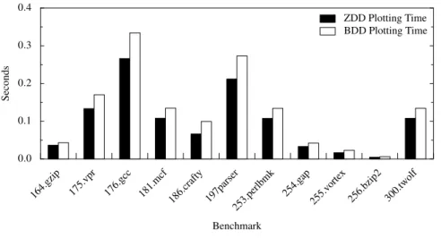
4.20 ZDD and BDD Visualization Time for SPEC INT 2000 benchmarks . . . 52
5.1 Computing a Reverse Slice using BDDs. [75] . . . 53
5.2 Computing a Reverse Slice using ZDD Unate Product. . . 54
5.3 Computing an Reverse Slice using ZDD ITE. . . 55
5.4 Computing an Reverse Slice using ZDD Intersection. . . 55
5.5 Slicing times . . . 57
6.1 Irrelevant Instruction Dependency Elimination Pseudo Code . . . 59
6.2 400.perlbench Instruction Dependencies Removed per Iteration . . . 60
6.3 401.bzip2 Instruction Dependencies Removed per Iteration . . . 60
6.6 445.gobmk Instruction Dependencies Removed per Iteration . . . 61
6.7 456.hmmer Instruction Dependencies Removed per Iteration . . . 61
6.8 458.sjeng Instruction Dependencies Removed per Iteration . . . 62
6.9 471.omnetpp Instruction Dependencies Removed per Iteration . . . 62
6.10 473.astar Instruction Dependencies Removed per Iteration . . . 62
6.11 483.xalancbmk Instruction Dependencies Removed per Iteration . . . 63
6.12 Total Irrelevant Instruction Dependencies Count for GCC -O0 . . . 63
6.13 Total Irrelevant Instruction Dependencies Count for GCC -O2 . . . 63
6.14 Total Irrelevant Instruction Dependencies Percentage for GCC -O0 . . . 64
6.15 Total Irrelevant Instruction Dependence Percentage for GCC -O2 . . . 64
6.16 Total Irrelevant Instruction Dependence Diff -O0 to -O2 . . . 64
6.17 Total Irrelevant Instruction Dependence Diff -O0 to -O2 . . . 65
6.18 DINxRDY plot of SPEC CINT 2000 benchmark 254.gap . . . 67
6.19 Selected Instructions for Dead-Ready Testα . . . 67
6.20 Region after Dead-Ready Test ofα . . . 68
6.21 Selected Instructions for Dead-Ready Testβ . . . 68
6.22 Filtered for Dead-Ready Testβ . . . 69
6.23 254.gap Filtered with Irrelevant Component Elimination . . . 70
6.24 254.gap with Highlighted Hot Code . . . 71
6.25 Selected Instructions for Dead-Hot Test . . . 72
6.26 254.gap Regionβ . . . 72
6.27 Dead-Hot Filtered Region . . . 73
7.1 Overview DINxRDY Plot of 175.vpr . . . 76
7.2 DINxRDY for Bad Region Selection (η) . . . 77
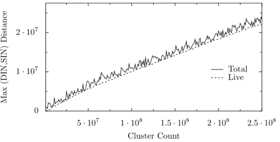
7.4 k-Means Clustering vs. Maximum DIN,SIN Distance . . . 79
7.5 Computing a Reverse Slice to Convergence using BDDs. . . 80
7.6 Computing a Single Reverse Slice using ZDDs. . . 81
7.7 Fixed-Point Slice Computation with ZDDs. . . 82
7.8 Computing a Single Forward Slice using ZDDs. . . 83
7.9 ZDD Chop . . . 84
7.10 ZDD Chop Illustrated . . . 84
7.11 Fine-Grained from Figure 7.12 . . . 85
7.12 Potential Parallel Code Example. . . 86
7.13 Fine-Grained from Figure 7.12 . . . 87
7.14 Coarse-and-Fine Grained from Figure 7.12 . . . 87
7.15 Coarse-Grained TLP and TLS [48] . . . 88
7.16 401.bzip2 with Selected Regions . . . 89
7.17 401.bzip2 -O0 and -O2 Functions with TLP . . . 90
7.18 Potential Coarse-Grained TLP . . . 92
7.19 Optimistic Thread Count . . . 93
7.20 Potential TLP W/0 Interdependent Instructions . . . 94
7.21 Maximum Threads W/0 Interdependent Instructions . . . 95
7.22 400.perlbench TLP with Synchronization . . . 95
7.23 400.perlbench with Selected Potential TLP . . . 96
7.24 400.perlbench TLP Source Code Region 1 . . . 98
7.25 400.perlbench TLP Source Code Region 2 . . . 99
7.26 400.perlbench TLP Source Code Lines Region 1 . . . 100
7.27 400.perlbench TLP Source Code Lines Region 2 . . . 101
7.28 445.gobmk with Selected Potential TLP . . . 101
7.29 445.gobmk Inter-Region Dependencies . . . 102
A.1 Tuple Relation Types . . . 118
B.1 400.perlbench with Selected Regions . . . 120
B.2 401.bzip2 with Selected Regions . . . 120
B.3 403.gcc with Selected Regions . . . 121
B.4 429.mcf with Selected Regions . . . 121
B.5 445.go with Selected Regions . . . 122
B.6 456.hmmer with Selected Regions . . . 122
B.7 458.sjeng with Selected Regions . . . 123
B.8 462.libquantum with Selected Regions . . . 123
B.9 464.h264ref with Selected Regions . . . 124
B.10 471.omnetpp with Selected Regions . . . 124
B.11 473.astar with Selected Regions . . . 125
B.12 483.xalancbmk with Selected Regions . . . 125
C.1 164.gzip DINxRDY with Hot Code . . . 127
C.2 175.vpr DINxRDY with Hot Code . . . 127
C.3 176.gcc DINxRDY with Hot Code . . . 128
C.4 181.mcf DINxRDY with Hot Code . . . 128
C.5 197.parser DINxRDY with Hot Code . . . 129
C.6 252.eon DINxRDY with Hot Code . . . 129
C.7 253.perl DINxRDY with Hot Code . . . 130
C.8 254.gap DINxRDY with Hot Code . . . 130
C.9 255.vortex DINxRDY with Hot Code . . . 131
C.10 256bzip2 DINxRDY with Hot Code . . . 131
D.1 400.perlbench DINxRDY with Hot Code . . . 134
D.2 401.bzip2 DINxRDY with Hot Code . . . 134
D.3 403.gcc DINxRDY with Hot Code . . . 135
D.4 429.mcf DINxRDY with Hot Code . . . 135
D.5 445.go DINxRDY with Hot Code . . . 136
D.6 456.hmmer DINxRDY with Hot Code . . . 136
D.7 458.sjeng DINxRDY with Hot Code . . . 137
D.8 462.libquantum DINxRDY with Hot Code . . . 137
D.9 464.h264ref DINxRDY with Hot Code . . . 138
D.10 471.omnetpp DINxRDY with Hot Code . . . 138
D.11 473.astar DINxRDY with Hot Code . . . 139
Instruction level parallelism (ILP) limitations have forced processor manufacturers to develop
multi-core platforms with the expectation that programs will be able to exploit thread level parallelism (TLP) [1–3].
This shift forces software engineers to try and improve the performance of their applications with
high-level redesigns focused on exposing parallelism, as well as explore aggressive optimizations for sequential
codes [39, 71]. Extracting TLP by manual high-level software redesign is often difficult [40]. Instruction
level dynamic program analysis can provide useful guidance for program optimization, including efforts to
find and extract thread level parallelism. However, optimizations often exist within large dynamic traces [44],
and finding opportunities for performance can require the analysis of gigabytes of trace data. This thesis
shows that: (1) Zero-Suppressed Binary Decision Diagrams (ZDDs) enables many analyses to scale; (2)
ZDD creation is practical for traces of a billion instructions for a variety of benchmarks; and, (3)
ZDD-based analysis, such as irrelevant instruction detection and potential coarse-grained thread level parallelism
extraction, can reveal a number of performance opportunities that exist in sequential programs.
1.1 Dynamic Trace Compression
Dynamic trace analysis has been used in prior work for performance tuning and hardware
debug-ging [102]. Unfortunately, trace files can easily grow to terabytes in size depending on the information
collected and the duration of traced execution. Large dynamic trace sizes (e.g. 1 billion instructions or more)
can make analysis and visualization impractical.
compress these traces by a factor of 10 or more. Unfortunately, these techniques do not speed trace analysis.
Compression techniques force analyzers to stream a decompressed version of the trace through the analysis
engine. Thus, analyses have complexity that depends on thedecompressed trace size, even though the
decompressed trace is never stored on disk. With large traces, this time-consuming process prohibits certain
global analyses and interactive tools. Examples of prohibitively expensive operations include memory-data
liveness visualization, hot code visualization, trace slicing [105], and interactive visualization of thread level
parallelism.
Ideally, a compressed trace format should allow analyses to operate directly on the compressed
representation with complexity that is a function of compressed trace size. Then, if large portions of
compressed traces fit in memory, global analyses and interactive visualization become possible. Laruset.
al. propose such a technique forwhole program pathanalysis [58]. The technique uses the SEQUITUR
compression method and works well for finding sequence matches in program execution. However,whole
program pathanalysis does not permit direct application of data-centric analyses (e.g., trace slicing) that are
of interest to system designers and programmers. Recent work on stride compression techniques addresses
this issue by forming hierarchies based on accessed memory regions [50], but is limited to analyses based on
loop-level dependence.
This thesis explores reduced, ordered, binary decision diagram (ROBDDs) [17], originally developed
for hardware verification, as a trace representation for dynamic program analysis. BDDs can provide
compression for large sets of data whose size would otherwise make analysis intractable. For example, BDDs
in hardware verification and validation allow equivalence checking of circuits with many states in constant
time [14]. In program analysis, BDDs have been used to store program contexts for each object in a program
analysis lattice object [99]. When BDDs are used for the analysis of large program traces [75, 78, 105], the
size of dynamic program traces can be reduced by up to 60x when encoded as a BDD [75]. Further, this
compressed representation can be analyzed without decompression, with algorithmic complexity that is a
function of the compressed size [75]. Thus, trace-encoded BDDs provide a solution to the dynamic trace size
Encoding large traces as BDDs can be time consuming, requiring hours to days to complete [77].
This in turn makes tools that use BDD-based representations less effective than otherwise possible. Prior
applications of BDDs depend on three methods to mitigate BDD creation time: (1) search for a variable order
that allows for fast BDD creation, (2) tune the tables and caching systems used in many BDD packages, and
(3) encode an abstraction of the original data set. This thesis discusses zero-suppressed BDDs (ZDDs) as
an alternative to BDDs in order to reduce creation time for large traces. Prior work has shown that ZDDs
can reduce the final BDD size for sparse data and context data used during static program analysis [43, 62],
though this work has not applied ZDDs to compressing dynamic trace data. This thesis shows that, without
data loss, ZDD-based SPEC INT 2000 benchmark traces are 25% smaller than BDD-based traces.
Traces from a variety of applications need be analyzed to demonstrate the efficacy of ZDD-based
dynamic trace analysis. Reducing trace creation time by 25%, which intuitively should correspond to the
25% reduction in representation size, is beneficial, but simply not enough to allow analysis of billions of
instructions from a variety of benchmarks. Initial tests of ZDD creation time proved to be far worse; the 25%
reduction in representation size did not translate to 25% reduction in creation time. ZDDs creation time was,
for some benchmarks,3×slower. Further investigation revealed a modification to the caching mechanism will remove this penalty in most cases. In fact, ZDD-based trace compression algorithms have a smaller
working set size making tuning possible for large traces, which results in a creation time that can be9×faster than BDD creation time for the same benchmark. A detailed discussion of ZDD-based trace compression can
be found in Chapter 4.
1.3 Opportunities for Optimization
Reducing ZDD creation time is crucial to explore opportunities for optimization in a wide range of
program traces. Chapter 7 explores potential coarse-grained thread level parallelism (TLP) that exists in
sequential applications. Chapter 6 demonstrates the use of ZDD-encoded traces to locate irrelevant instruction
Irrelevant Instruction Elimination
Irrelevant component elimination has been used in prior work to simplify abstractions for static
analysis [23]. This thesis uses an irrelevant component elimination with ZDD-encoded precise dynamic
instruction dependencies. This thesis will show that ZDD-based irrelevant instruction dependency elimination
can locate instructions that fail to the following criteria: (1) the instruction dependence chain should reach the
end of the program trace; or, (2) the dependence chain should produce an output through a Linux system call.
ZDD-based irrelevant instruction dependency elimination is designed to iterate irrelevant code
calcula-tion until convergence. However, irrelevant instruccalcula-tion dependency eliminacalcula-tion can take days to complete
for traces with long dynamic dependency chains. Empirical data presented in this thesis shows that, for all
benchmarks in SPEC 2006 INT, the irrelevant instruction elimination algorithm reaches a steady state. In this
state, the number of instruction dependencies removed per slice iteration oscillates, but will not monotonically
decrease until the analysis converges. Thus, it is possible to approximate the number of instructions removed
by iterating irrelevant instruction elimination until oscillation is detected.
ZDD-based irrelevant instruction dependency elimination may also be used to filter irrelevant points
from program visualizations. However, irrelevant instruction dependency elimination may also be used
as a technique for code optimization or compiler evaluation. Chapter 6 contains a survey of irrelevant
code removal from the SPEC 2006 INT benchmarks using both-O0and-O2optimization levels in thegcc
compiler.
Hot-Code Visualization
In addition to the optimization analyzes presented in this thesis, which include coarse-grained thread
level parallel region location and irrelevant instruction elimination, a hot-code visualization algorithm was
created to focus optimization efforts on the most frequently executed regions of code.
Hot-code analysis captures static instruction execution frequency and counts the frequency of
ex-ecution. The static hot code information is combined with a mapping from dynamic instruction → static instructionsto create a new relation from each dynamic instruction to hot-code value. The resulting visualizations can be found in Appendix C and Appendix D.
Traces from a variety of applications need be analyzed to demonstrate the efficacy of DD-based
dynamic trace analysis. The results in this thesis show that ZDD-based trace compression results in 25%
smaller representation compared to BDD-based traces. Further, ZDDs have a smaller working set, thus the
ZDD creation package can tuned to cache the working set of the trace-ZDD during creation. This reduces the
number of garbage collection operations and removal of useful dead nodes. This reduces DD creation by up
to 9×.
Hot code analysis can tell developers where to focus optimization and parallelization efforts. In
addition to the optimization analyzes presented in this thesis, which include coarse-grained thread level
parallel region location and irrelevant instruction elimination, a hot-code visualization algorithm was created
to focus optimization efforts on the most frequently executed regions of code.
The results from a survey of irrelevant instructions in the SPEC 2006 INT benchmark shows that over
50% of instruction dependencies do not produce a value and do not reach the end of the program trace. It
is possible for an instruction to be relevant to program execution but not meet the specified requirements.
Therefore, this thesis also presents results comparing the irrelevant dependence counts from both the-O0and
-O2compiler settings. The irrelevant dependency count from the-O0, or non-optimized, compiler setting
provides a worst-case value to normalize further comparison operations. Furthermore, this technique can test
the effectiveness of static compiler optimizations, as well as locate potential irrelevant instruction streams.
This thesis explores potential coarse grain TLP that may be exploitable in conjunction with TLS
and ILP techniques. In particular, the thesis examines the SPEC INT 2006 benchmark suite, looking for
parallelism with a granularity of thousands of dynamic instructions, and is not restricted to loop-level TLP.
The survey presented in Chapter 7 found, on average, 7% of instructions may be extracted as course-grained
parallelism, and for the benchmark 445.gobmk, 44% of instructions may be extracted as coarse-grained TLP.
Potential Coarse-Grained Thread Level Parallelism
An effective, popular, and widely studied mechanism for automatically exploiting parallelism is to
advances in this thread level speculation (TLS) can parallelize execute over 90% of some codes [64]. However,
TLS predictor accuracy limits TLS to fine-grained or loop-level TLP [15, 64, 79, 90, 98].
This thesis explores potential coarse grain TLP that may be exploitable in conjunction with TLS
and ILP techniques. In particular, the thesis examines the SPEC INT 2006 benchmark suite, looking for
parallelism with a granularity of thousands of dynamic instructions, and is not restricted to loop-level TLP.
Coarse-grained TLP is located using the ParaMeter dynamic trace visualization tool [78]. This technique,
which is discussed in Section 7.1, generates a visualization of program execution, called a DINxRDY
(dynamic instruction number by ready time) plot. This plot visually shows potential coarse grain TLP as
lines that overlap on the x-axis.
Potential parallel regions found within DINxRDY plots are further analyzed to expose dependence
relationships. Inter-region dependence conflicts, discussed in Section 7.4 are found by dynamic dependence
graph (DDG) slicing [4, 5, 30, 52]. Slicing DDGs that contain a large number of instructions (e.g. billions) can
take weeks [5,104]. To efficiently, and precisely, explore the dependency relationships between two regions of
code this thesis extends the DDGchopto use the ZDD-compressed trace format. The dynamic chop [36, 54]
is often faster than an intersection of a forward and reverse slice and requires no loss of precision.
The survey presented in Chapter 7 found, on average, 7% of instructions may be extracted as
course-grained parallelism, and for the benchmark 445.gobmk, 44% of instructions may be extracted as
coarse-grained TLP.
Finally, a summary of contributions, techniques, and results of this thesis may be found in Chapter 9.
Thus, this thesis presents the following contributions:
(1) A ZDD-based trace compression algorithm with tuning for large traces, resulting in a 25% reduction
in BDD size and a9×reduction in trace compression time.
(2) A ZDD-based iterative analysis for locating irrelevant instruction dependencies
(3) A method to quickly explore coarse-grained parallelism in serial applications.
up to 44% of instructions may be extractable as coarse grain TLP.
1.5 Hypothesis
ZDD-based dynamic trace analysis can identify hot-code paths, irrelevant instructions, and potential coarse-grained thread level parallelism in sequential codes, and thus create opportunities for program optimization.
Chapter 2
Parallel Computation Background
Parallel computation is a source for performance for both software and hardware in many modern
computer systems [1–3]. Correct manual thread level parallelization of software can be difficult, may result in
non-deterministic errors, and often the resulting parallel application is often harder to debug than a sequential
application [29, 40, 57]. This thesis explores software tools that help a developer find and extract parallelism.
Parallel computation and parallel programming would require volumes to discuss completely [40, 61]. This
thesis requires an understanding of three attributes of parallel tasks: (1) location; (2) granularity; and, (3)
conflicts. Prior works have researched both automatic and manual techniques for defining the location,
granularity, and conflicts in potential parallel tasks. Following a discussion on these topics, this chapter will
then explore static and dynamic techniques that can locate parallel tasks and task conflicts.
2.1 Automatic Parallelization Techniques
Automatic parallelization is a heavily research field [38, 41, 95]. Parallel task location and granularity
are defined by instructions contained within a parallel task boundary [19]. Conflicts between parallel tasks
often occur from read-after-write hazards; if a task alters a value read by a different parallel task can result in
unexpected program execution. This section looks at static and dynamic techniques for automatically finding
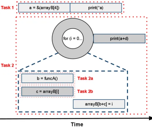
2 : f o r ( i = 0 ; i < a r r a y B . s i z e ( ) ; ++ i ) 3 : { 4 : b = funcA ( ) 5 : c = a r r a y B [ i ] 6 : a r r a y B [ b + c ] = i 7 : } 8 : p r i n t (∗a ) 9 : p r i n t ( b )
Figure 2.1: Parallel Pseudo Code Example
2.1.1 Automatic Parallelization by Static Analysis
The location of parallelism can be determined a statically before program execution by a compiler [16,
25]. The example code in Figure 2.1 can help explain how to find parallel tasks and task boundaries using
only static program information. An illustration of the sequential execution of the source in Figure 2.1 can be
seen in Figure 2.2. This code is in C/C++ style, and contains many pointer operations to demonstrate the
limitations of some analysis methods. In line 1, the variableais a integer pointer variable, and the arrayB
contains integers. Thus, line 1 sets the value ofato a pointer to the fourth member of arrayB.
The next point of heap obfuscation occurs inside the control flow test in line 2. The functionsizeis a
member of the array type used in this pseudo code. This function determines the size of the array, which can
be difficult to determine at run-time. Thus, a static analysis would likely need to becontext sensitiveand
interprocedural. Context sensitivity allows the analysis to understand the difference, or similarities, between
multiple occurrences of the same static code [28]. An interprocedural analysis allows the analysis to go into,
and out from, a function call during analysis [8]. A context sensitive and interprocedural analysis would still
need to determine the size of the arrayarrayBwhich was likely allocated using heap memory. In languages
that allow heap allocation and references, the size and value of heap memory is difficult to determine at
compile-time difficult [51, 66, 92].
with a run-time input, than the size of the array could not be found by static analysis. Interprocedural static
analysis, such aspoints-to[86] andalias[22] can find conflicts between instructions.
The final heap accesses in the pseudo code in Figure 2.1 occur in lines 5 and 6. The heap read in linec
= arrayB[i]would a points-to analysis to disambiguate. The next line,arrayB[b + c] = i, is a write to a heap
memory location. If a static analysis can find the exact location of the memory write, then it is possible to
perform additional parallelization analyses. However, the heap write access location is the combination of a
function return value and the value in another heap memory location. It is likely that a static analysis would
need to classify this memory write location as all possible heap location values, ortopusing a lattice that also
represents the empty set∅asbottom[24, 89]. Top may also be written as>, and bottom may be seen in this thesis as the symbol⊥. If line 6 in Figure 2.1 is found to be>by a static analysis, it will cause line 6 to conflict with all other heap memory writes, and add line 6 to the dependence chain of a heap memory read.
Thus, line 6 would become difficult to parallelize using static auto-parallelization.
The example code also contains potential parallelism that is not bounded by a programming construct.
For example, if the value ofb + cin the linearrayB[b + c] = iis less than four, than the instructions a =
&(arrayB[4])followed byprint(*a), and the loopFor (i = 0; i ¡ arrayB.size(); ++i)may be able to execute
in parallel. This program execution is shown in the illustration in Figure 2.4.
Figure 2.3 contains an illustration of the execution of the pseudo-code in Figure 2.1 using
medium-to-fine grained parallel tasks bounded by control flow constructs. This illustration assumes a static, likely
points-to, analysis finds that line 6 does not alter the heap locations read by line 5. Even if this is not
the case, and line 5 depends on a value written by line 6, it may still possible to create parallel software
pipelines [32, 81].
Figure 2.1 demonstrates how the boundary of parallel tasks located by static analysis can be limited by
control paths that are resolved at run-time [95]. Prior work has found that even state-of-the-art automatic
parallelizing compilers are often unable to parallelize simple embarrassingly parallel loops written in
Figure 2.2: Sequential Execution of Program in Figure 2.1
2.1.2 Automatic Parallelization by Dynamic Analysis
Dynamic auto-parallelization techniques examine the run-time execution of a program, and thus can
see how control flow dependencies are resolved. This illustration in Figure 2.4 show the pseudo-code in
Figure 2.1 could be parallelized if a dynamic analysis were able to extract all potential parallel instructions.
Note that the fine grained parallel tasks from Figure 2.3 are still executed as parallel tasks in Figure 2.4
spawned from Task 2.
An illustration of dynamic execution of the pseudo code in Figure 2.1 is shown in Figure 2.5. Thefor
loop from the static code is shown partially unrolled in the the dynamic execution illustration.
Parallel tasks found by a dynamic analysis are only correct for the program input, or the set of inputs,
that have been analyzed. Therefore, to ensure correct execution, thread-level parallelism found and executed
dynamically is often executed speculatively. There are many works exploring thread-level speculative (TLS)
techniques [20, 25, 69, 82, 87, 93, 97, 98, 101]. This thesis does not require a detailed understanding of
transactions and speculation, but basic concepts are necessary. If two tasks are executed speculatively, then,
for this work, it is assumed that the program executed in such a way that the final program state is identical to
that of the sequentially executed code.
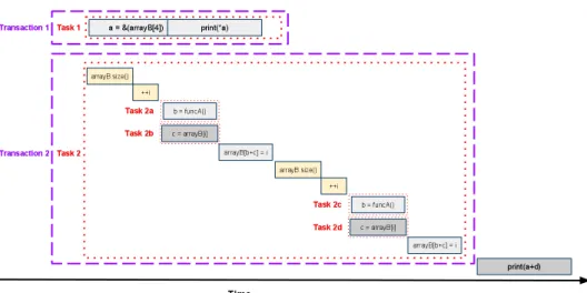
The illustration of the pseudo code in Figure 2.1 contains the dynamic code execution with TLS from
Figure 2.5. The regions of this illustration contained byTransaction 1orTransaction 2may be rolled back
by our hypothetical TLS system. Note that this illustration does not include nesting TLS; this is also true for
many research TLS systems [74].
TLS often incorporate prediction to extract additional parallelism [48]. Prediction systems used by
TLS can speculate values, control directions, and data dependencies. Figure 2.7 shows an illustration of a
TLS system using control prediction to execute each iteration of theforloop in parallel. Value prediction in
Figure 2.7 also allows the value ofi, which is read by instructions inside theforloop, to be predicted and
propagated.
The illustration in Figure 2.6 can help explain why TLS is often most effective when extracting threads
Figure 2.4: Static Fine-to-Coarse Grained Parallel Tasks from Figure 2.1
Figure 2.6: Dynamic Coarse Grained Parallel Tasks from Figure 2.1 with TLS
403.gcc 14.14 429.mcf 17.7 445.gobmk 12.78 456.hmmer 0.1 458.sjeng 16.1 462.libquantum 0.1 464.h264avc 3.34 471.ommnetpp 15.5 473.astar 40.67 483.xalancbmk 9.1
Figure 2.8: Performance from TLS [48]
conflict, thenTransaction 2will likely roll back the entire transaction. Complex tasks may increase the risk
of misprediction by including more predicted values, dependencies, and branch directions [64]. Work by
Raviet. al.looks at a technique based on transactional memory to expand TLS to coarse-grained threads, but
is limited to scientific codes with regular access patterns [80]. TLS has been applied to C and Java objects that
contain thousands of instructions, but work by Warget. al.found limited gains were realized from objects
with more than 100 instructions [98].
TLS can greatly improve program performance, regardless of the granularity limitations. For example,
TLS performance gains from a TLS system that uses perform control, data dependence, and data value
speculation [48], are shown in Figure 2.8.
2.2 Parallelization with Tools
Automatic parallelization is difficult, and most successes are limited to highly numeric applications [60,
80]. This section examines tools that can help a programmer find potential parallel tasks and find potential
task conflicts. Static parallelization tools have had some success [49], but are ultimately limited in the
presence of pointers and dynamic memory allocation [50]. This section explores tools that use run-time
program information, much like TLS, for finding potential parallel tasks and task conflicts.
keep the science behind these systems a secret [21, 94]. A limited number of tools have recently emerged
from the research community, and are easier to explore for this section.
Alchemist is a dynamic profile based tool that locates potential parallelizable regions at run-time.
Dependence conflicts are also located and presented to a user for manual parallelization [106]. The Alchemist
tool restricts parallel tasks to regions bounded by artificial constructs, likeif-than-elsebranches or loops.
Recent research into parallel extraction tools include SD3 [50], Parkour [45], and Kremlin [31]. The
SD3 tool performs inter-region dependence analyses similar to those discussed in this work. The regions
located by SD3 are defined stride-compression, and therefore are generally limited to locating potential
parallelizable regions in loops. Many recent advances in parallel task boundary locations are also limited to
parallelism bounded by explicit constructs [31, 45].
Most tools that use dynamic program information to aid parallel programming are restricted to parallel
tasks that can be bounded byif-than-elseblocks,fororwhileloops, or function calls [31, 45, 50, 106]. This
limitation is likely in place for the following reasons: (1) it is unclear how to find task boundaries without
constructs; (2) constructs help trace compression; and, (3) frequently executed code blocks are often contained
inside loops.
Constructs Create Boundaries
Artificial constructs are an easy way to define a parallel task boundaries. If the user defined a task to be
contained in a function call, than that parallel task should be easy for the user to identify. Using techniques
prior to the work in this thesis, it is not clear how to define the boundaries of these parallel tasks [31, 45].
Further, some works include the “ease of thread extraction” in calculations for deciding if a task is worth
parallelizing [31]. Unfortunately, there may be groups of instructions that could be a parallel task, but are not
contained by a construct in the static code.
Constructs Help Compression
Dynamic program analyses often need some dynamic information to be visible for the life of the
program execution. Dynamic trace information can grow very large (e.g. gigabytes), and requires some form
of analyzable compression. A potential parallel task that is bounded by a static construct can be stored for
only instances of the static code requires much less space than a trace of the dynamic execution, but at the
cost of a loss of precision and flexibility. For example, if the tool stores only static data than it would be
difficult to know how many times that region of code was executed. The execution count can be valuable for
finding hot code regions. If the tool also includes an execution count number per static region, there is likely
some additional data lost that could become useful in the future. The process of creating an abstraction of
the dynamic execution by storing only static data and limited contexts limits future analysis to what may be
performed using only data the original tool designer found to be relevant.
Constructs Define Hot-Code
The Kremlin tool [31] can find parallel tasks, and generates metrics for the ease of extraction, and
the frequency of execution. The ease of extraction metric is mostly a reflection of the number of potential
conflicts. The frequency of execution value can help the user focus parallelization efforts only highly executed,
or hot, regions of code. Loops created byfororwhileconstructs are often the source of hot code regions [12].
However, a loop may contain an expensive operation, such as memory allocation or file IO, and may not
be executed frequently. Furthermore, a loop may contain instructions that are worthy of parallelization, but
are included in a loop that also may conflict with another parallel task. Conflicts make tasks difficult to
parallelize; some tools and may reduce the value of a potential parallel task with conflicts, or eliminate such
tasks altogether [31].
This thesis presents a system for finding, analyzing, and extracting potential parallel regions from serial
codes. The tool presented by this thesis can be used to quickly develop dynamic traces analyses. The trace
compression developed for this thesis allows for off-line analysis, thereby allowing new analysis to quickly
be tested and executed on a benchmark suite, without the additional step of re-running each benchmark. In
fact, the ability to quickly develop new analysis allows this system to be rapidly adapted to new tasks, such as
finding irrelevant code in dynamic traces. For modern multi-core systems, the work in this thesis can find
Chapter 3
Related Works
This chapter presents work relevant to this thesis. Trace compression, visualization, and analysis are
examined in this chapter. Decision diagram (DD) construction techniques are also discussed.
3.1 Dynamic Trace Compression
Managing large dynamic traces is the key problem when performing whole program analyses. Consider
that 1 billion 64bit values need≈7.5 GB of uncompressed storage and that traces usually contain billions of instructions (10-1000s of GB). Therefore, any trace analysis tool must operate on compressed data. Further,
analyzing this data many need either sequential or random access mandating different compression techniques.
ParaMeter requires rapid random access coupled with good compression.
Researchers have used three methods to reduce trace sizes: (1) abstraction; (2) compression by
predictor-based encoding; and, (3) compression by program structure exposing methods, such as run-length
encoding or hierarchical grammars. Stride-based compression techniques have recently emerged as a viable
option for some analyses, such has hot-code and memory-conflict location [50].
3.1.1 Abstraction and Elimination
Data abstraction creates an abstract representation for concrete data. Abstract representations can be
more compact and easier to analyze. For example, some abstractions applied to concrete dynamic trace data
include, but are not limited to, a mapping from instructions to object creation/destruction [85], or program
designer. For example, the whole program path (WPP) trace representation [58] aggregates data from multiple
occurrences of the same program path. However, information that is difficult to aggregate, like cache misses
or CPU temperatures, will be removed from the WPP representation.
3.1.2 SEQUITUR Compression
The Sequitur compression algorithm is useful for compressing instruction level dynamic traces into an
analyzable representation [67]. However, while Sequitur can rapidly provide an analysis with information
about the instruction sequences in a trace, specific instruction information often requires an expensive traversal
of the grammar. Do demonstrate grammar creation, lets generate a grammar for the following sequence of
letters:
abcdabcdabc
We begin by creating a start rule:
S →abcdabcdabc
Sequitur forms a grammar online, thus the algorithm would first detect the repetition of the variablesab. The algorithm then creates a new ruleA→ab:
S →AcdAcdAc
A→ab
This processes is repeated forAc, thereby forming a hierarchical grammar:
S →BdBdB
A→ab
B →Ac
This processes is repeated forBd:
S →CCB
A→ab
B →Ac
3.1.3 Sequential Compressed Traces
Burtscher et. al.[18] in 2005 described a predictor based strategy requiring only mispredictions
to be stored in the trace file. The resulting compressed trace file is further compressed with a standard
stream compressor such as gzip or bzip2 achieving a 10 times compression factor with rapid streaming
decompression. Generating interactive DINxRDY plots from such stream compressed data is impractical
as the data must be entirely decompressed for each frame,≈ 1minute on a 2.0 GHz Pentium 4 for each 800x600 pixel plot in a trace containing only 100 million instructions. Worse, selecting and performing
slice analysis on instructions requires two additional passes through the complete data set adding another 2
minutes to the frame’s render time.
Work by both Iyeret. al.[44] and Zhang et al. [105] addresses this problem by generating intermediate
representations. Iyer’s work maintains a stream compressed intermediate representation suitable for working
on the current frame, but leaves the navigation problem unsolved. Zhang et al. [105] use a BDD to maintain
theintermediate analysisresults in a compact form in RAM. However, the navigation problem, as well as
inquiries into the contents of a DINxRDY plot, is still prohibitively expensive.
3.2 Reduced Ordered Binary Decision Diagrams
Reduced, ordered, binary decision diagrams (BDD) were first described by Akers [6] and further
developed by Bryant [17]. BDDs have been used in many domains including hardware verification [14],
cryptography [53], static program analyses [56, 100], and some use in dynamic trace analysis [105].
BDDs can be viewed as compressed versions of binary decision trees. Figure 3.1(a) shows a binary
tree for the three variable functionf(x, y, z) =x0y+xy0 +z. For example, traversing the left edges of the graph we evaluatef(0,0,0)as0. BDDs are a graph data structure in which each node corresponds to a Boolean function (just as each node in a binary decision tree) [17]. The following two reduction rules are
used to convert a decision tree to an BDd:
(1) When two BDD nodespandqare identical, edges leading toqare changed to lead topandqis
X false arc inverting false arc true arc Y Y Z Z Z Z 0 1 1 1 1 1 0 1
(a) Binary Decision Tree
X Y Y Z 1 (b) Na¨ıve Order Z Y X 1 (c) Better Order Figure 3.1: A Three-variable Binary Decision Tree and BDDs
(2) If both edges from a nodepgo to child nodeq, thenpis eliminated and all nodes that go topare
redirected toq.
The last reduction rule is commonly referred to as theS-deletionrule [43]. Figure 3.1(b) shows the
BDD forf under the variable ordering(x, y, z)with additional compression provided by inverting edges. To computef(0,0,0)with the BDD, we traverse the0, or false, arc of the X node, the false arc of the rightmost Y node and the inverting false arc of the Z node. Because we reached the constant1node through an odd number of inverting arcs, we findf(0,0,0) = 0as before.
3.3 Zero-Suppressed Binary Decision Diagrams
For this research I propose using BDDs to represent sets of dynamic program trace information. The
Boolean function that describes the inclusion of a set in a Boolean function is called the characteristic
function. BDDs can perform many set operations efficiently [17].
However, Minato [42] found that BDDs were inconvenient for sets of binary vectors. The tuple based
dynamic trace encoding method used by this proposal employs a variation of this binary vector encoding
technique. Specifically, a Minato creates sets of combinations of objects represented by a binary vector,
(xnxn−1xn−2...x2x1). In this vector each bit represents the inclusion of the object in the set. Using BDDs,
each bit in the binary vector and a variable in the Boolean formula. The size of a BDD depends on the number
of variables in the encoding, as well as the variable order. Therefore, it is useful to know the smallest number
of relevant bits in a bit vector before performing BDD encoding. Unfortunately, it is not always possible to
know the smallest number of relevant bits for a bit vector.
The following example better illustrates this problem: The vector0101has four bits. If the rightmost bit is the least significant bit, then, in this case, let us assume only the rightmost three bits are actually useful.
It is possible to encode this vector in a BDD with three variables, representing the vector101. However, imagine this operation101∧1101. The BDD must not contain four variables, but Boolean algebra states the vector101contains adon’t carevalue for the fourth bit, which is not correct. Thus, the BDD should be built with a variable for each potential bit in the bit vector.
Y Y
Z Z
0 1 1 1
Figure 3.2: A ZDD forf(x, y, z)
Minato [42] proposed a variation on BDDs, called ZDDS, to address this issue, and to reduce the size
of BDDs for sparse data sets. ZDDs are a variant of BDDs where theS-deletioncompression rule is replaced
by the use of thepD-deletioncompression rule. In this section we see that ZDDs provide better compression
than BDDs for trace data, and over9×faster creation times.
Zero-suppressed BDDs, or ZDDs, replace theS-deletionrule with thepD-deletionrule. This rule
states the following:
• If the1edge from a nodepleads to a zero terminal node and whose0edge a child nodeq, thenpis eliminated and all nodes that lead topare redirected toq.
Furthermore, ZDDs do not typically implement the inverting arcs optimization, i.e., ZDDs have no
inverting arcs, only plainthenandelsearcs. To see how this rule change results in a different decision diagram, consider, once again, the functionf(x, y, z)whose binary decision tree was shown in Figure 3.1a. Figure 3.2 shows the ZDD for this function. For this function, ZDDs perform worse than BDDs, as most of
the values for(x, y, z)cause the function to evaluate to 1. However, for sparse functions (i.e., those with few 1’s in the range), such as trace data, ZDDs provide superior compression.
1
2
3
4
5
1 2 3 4 5
DIN
RDY
(a) As Captured1
2
3
4
5
1 2 3 4 5
DIN
RDY
(b) Ideal ScheduleFigure 3.3: Basic DINxRDY Plot with 5 instructions.
3.4 Hot Code Analysis
Ammonset. al.found that hot code regions often occupy less than 28% of the overall program code,
resulting in up to 98% of level one cache misses [10]. Therefore, hot code information can tell programmers
where to focus parallelization efforts. Using Sequitur-based trace representations, hot path information can
be generated by recursively summing the number of occurrences of sub-rules in a grammar [58].
3.5 Dynamic Trace Analysis
Dynamic traces information consists of information collected from a program at run-time. Software
developers can use instruction level dynamic trace analyses to create a picture of their software’s run-time
behavior, as well as software debugging [103]. However, dynamic traces can grow quickly in size (gigabytes
to terabytes) for seconds of program execution. Analysis of large quantities of data can be impractical using
commodity hardware [83].
3.6 DINxRDY Visualizations
Though parallelism found in prior studies [11, 55, 96] is not accessible to ILP techniques [96], it may
yield to thread level parallel (TLP) techniques. The Dynamic Instruction Number vs. Ready-time (DINxRDY)
plot (originally introduced by Postiff et al. [72]) can be useful in identifying the potential TLP inherent in
Consider the hypothetical 5 instruction trace shown in Figure 3.3(a). The vertical axis represents the Dynamic
Instruction Number (DIN) and the horizontal axis represents the earliest time at which an instruction can be
scheduled (ready-time, RDY). For example, Figure 3.3(a) shows that the 3rd instruction in the trace (dynamic
instruction 3, or DIN 3) was issued in cycle 3. Figure 3.3(b) shows the same trace under an ideal schedule
(i.e., one cycle per instruction, perfect branch prediction, infinite hardware resources, etc.) that respects all
data dependencies. This plot shows that DIN 3 is dependent on DIN 2 which in turn is dependent on DIN 1.
Further, the plot shows that DIN 4 is not dependent on DINs 1, 2, or 3 because it is scheduled in the first
cycle. Dependency analysis is needed to decide whether DIN 5 is dependent on DIN 1 or 4.
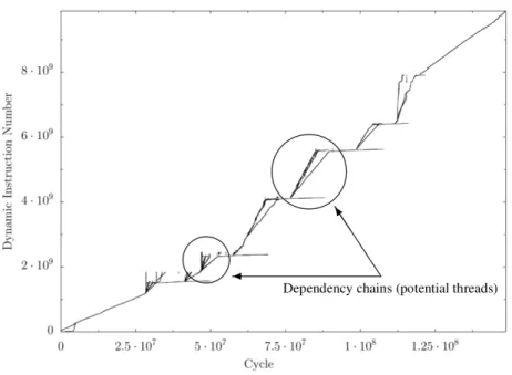
Iyer et. al. observed that lines running from lower left to upper right in DINxRDY plots form
dependency chains of relatively nearby instructions in a program [44]. Further, diagonal lines that have
overlapping x-extents suggest regions of code that might be convertible to TLP. Figure 3.6 shows a DINxRDY
plot for 254.gap with groups of divergent dependency chains (DDCs) (circled in the figure) suitable for TLP
extraction analysis. From Iyer’s work [44], we know that these suggest the presence of either data parallelism
or pipeline parallelism.
The Dynamic Instruction Number vs. Ready-time (DINxRDY) plot (originally introduced by Postiff
et. al.in 1998 [72]) can be a useful in identifying the potential TLP inherent in many sequential applications.
The dynamic instruction number (DIN) is a unique number assigned to each instruction when the instruction
executes at run-time. A single static instruction can execute many times during program execution and each
occurrence of that static instruction would generate a new DIN. The relation fromSIN → DIN is also stored.
This thesis uses sets{DINi,{DINd}}for program analysis. TheDINi → {DINd}relation, also
referred to as DINxDIN in this thesis, maps an instructionDINito a set of instructionsDINd. The members
of the setDINdhave a dependency that is resolved by dynamic instructionDINi. Thus, it is possible to
use theDINi →DINdto identify dependency relationships and perform dependence slicing. A full list of
Figure 3.4: Dynamic instruction number vs. ready-time plot of SPEC INT 2000 benchmark 254.gap. Circled areas represent potential threads
Numerous works have used dynamic program trace slicing, introduced by Korelet. al.[52], to explore
program behavior at run-time. Dynamic slices have been developed for locating the source of observed
program bugs [5, 91], program testing [30] and software maintenance [47]. Dynamic traces can quickly grow
in size beyond what can be stored and analyzed on commodity hardware [5, 75, 103]. Generating slices from
large dynamic traces can require days of computation time [5]. To reduce slice times, this thesis extends the
prior use of dependence chopping [36, 54].
Zhanget. al. first explored slicing with BDDs [105]. In the work by Zhang, program slice information
for each instruction is generated from the dynamic trace information. A variation of technique used to create
program slices is also used for the work in this thesis.
3.6.2 Hot Code Analysis
Hot code analysis can tell developers where to focus optimization and parallelization efforts. Ammons
et. al.found that hot code regions often occupy less than 28% of the overall program code, resulting in up to
98% of level one cache misses [10]. Therefore, hot code information can tell programmers where to focus
parallelization efforts. Using Sequitur-based trace representations, hot path information can be generated
by recursively summing the number of occurrences of sub-rules in a grammar. Using BDD-encoded traces,
hot code information is generated directly from the program execution by maintaining a count of each static
instruction’s occurrence in the dynamic trace.
3.7 Parallelism in Computing
Until recently, software engineers could gain performance by waiting for processor core performance
to improve. However, manufacturers have been unable to extract performance from uni-processor designs,
forcing a trend towards multi-core systems [88]. Tasks can be parallelized using a variety of scopes:
• System Parallelism
• Thread Level Parallelism
• Instruction Level Parallelism
With the advent of compute cloud infrastructures, tasks that may be parallelized among systems can
be expanded (or reduced) depending on demand [68]. Application parallelism exists if there is a need, or
desire, to run multiple applications at the same time on the same operating system. Thread level parallel
distributes work between regions of the same program, with no programmer stated total order between
regions. Programmers can state an explicit order using synchronization methods such as locks, mutexes or
transactions [35, 59].
Limit studies during the 1990s showed that sequential applications have considerable potential
paral-lelism [11, 55, 72, 96] that is amenable to thread level paralparal-lelism (TLP) [44] but is not accessible via hardware
instruction level parallel techniques (ILP) [96]. Therefore, the proposed research will focus on software
4.1 BDD Compression Time
To understand why BDD-based compression is time consuming, this section begins by first describing
BDD-based trace representation [75]. This section then analyzes the BDD-trace creation algorithm and shows
that inefficient trace BDD compression is primarily caused by:
• Frequent garbage collection of dead BDD nodes
• The deallocation of potentially reusable dead BDD nodes and corresponding BDD system cache entries
4.1.1 Traces as Boolean Functions
BDDs represent boolean functions, and thus, to represent traces as BDDs, let us review how to
represent trace data as a boolean function [75].
Observe that boolean functions can encode arbitrary binary data. For example, if the represented
universe,Ω, consists of 4 elementsΩ ={a, b, c, d}, then a 2-bit encoding can be used to represent each element,{a7→00, b7→01, c7→10, d7→11}[75]. It is possible to create a boolean indicator function (i.e., characteristic function) that evaluates to true for any subset of theΩwith this encoding. For example, the indicator function for the set{a, b}isI{a,b}=x0wherexis the variable for the most-significant bit (MSb)
It is possible to extend this simple notion to encode different data sets necessary for representing and
analyzing the trace. All trace data is encoded by a set of tuples(DIN, data)where the DIN is the dynamic instruction number (i.e., the position in the trace, the first instruction has DIN 0, the second DIN 1, and so on).
Therefore, a simple instruction trace is encoded as(DIN, P C), where the PC is the program counter value. Similarly, more complex data relationships can be encoded by simply joining the binary representations of
arbitrary tuples into a single equation.
This chapter uses three types of data tuples. The first is(DIN, SIN), where theSINis the static instruction number orP C (Note that this thesis will useP C andSINinterchangeably). The second tuple type is(DIN, DIN), which is used to represent edges of the trace’s dynamic data dependence graph. If a decision diagram (DD) encodes an edge setE, if(10,24)is in the edge set then the 24th instruction in the trace depends on the 10th instruction in the trace. If we wish to know theP C of either of these instructions, we can refer to the(DIN, SIN) tuple set. Finally, this thesis evaluates(DIN, RDY)tuple sets, which encode the ideal schedule for the trace, i.e., for eachDIN,RDY is the earliest time a scheduler could execute thatDIN given an ideal machine [78]. A description of all tuple members and relation types can be found in Appendix A.
4.1.2 Boolean Functions as BDDs
BDDs can be viewed as compressed versions of binary decision trees. Figure 3.1(a) shows a binary
tree for the three variable functionf(x, y, z) =x0y+xy0 +z. For example, traversing the left edges of the graph we evaluatef(0,0,0)as0. BDDs are a graph data structure in which each node corresponds to a boolean function (just as each node in a binary decision tree does) [17]. A full discussion of BDD creation
can be found in Chapter 3, but for clarity the two reduction rules for converting a decision tree to an BDD are:
(1) When two BDD nodespandqare identical, edges leading toqare changed to lead topandqis
removed
(2) If both edges from a nodepgo to child nodeq, thenpis eliminated and all nodes that go topare
BDD forf under the variable ordering(x, y, z)with additional compression provided by inverting edges. To computef(0,0,0)with the BDD, we traverse the0, or false, arc of the X node, the false arc of the rightmost Y node and the inverting false arc of the Z node. Because we reached the constant1node through an odd number of inverting arcs, we findf(0,0,0) = 0as before. BDD creation is covered in more detail in the literature [17, 75, 84].
4.1.3 BDD Unique Tables
Prior work shows how to encode trace data as BDDs. However, the encoding processes can take an
unreasonable amount of time. Inefficient encoding is primarily caused by the interaction of garbage collection
and BDD system caches, specifically the unique table and the operation cache.
TheS-deletionrule used to reduce a binary tree into a BDD is realized through theunique table. The
unique table enforces strong canonicity because each new node has a unique location in the table. If a node
is a duplicate of an existing table node (i.e., it represents the same boolean function), the node is reused
from the unique table [17]. The unique table also increases the efficiency of BDD creation. If a BDD node
already exists the BDD management system, such as CUDD [84] (a state of the art, high-performance, BDD
package), saves time by reusing the existing node and avoiding re-computation for the remainder of the nodes
below the cached one.
The unique table can be used to tune the overall creation time of the BDD by altering its size. The size
of the unique table must at least be large enough to contain all of the live BDD nodes. With CUDD, however,
nodes contained in the subtable can also be dead. Upon garbage collection, these dead nodes are added to
death row, which is an additional cache used to hold recently invalidated nodes. The nodes on death row can
also be resurrected and reused.
In addition to a simple node cache, BDD packages, including CUDD, also have an operation cache
that caches the results of BDD operations. For example, if one requests a computation ofB ∧Cand the result isA, then CUDD will cache thatA=B∧C. IfB∧Cis requested again, it will immediately return BDDAfrom this cache, and perform the potentially exponential recursion required to recomputeA. This
cache gives BDDs their polynomial time complexity [17].
Unfortunately, garbage collection frees the nodes on death row in order to free memory, which, in turn,
evicts corresponding results from the operation cache. As we will see, the eviction of useful results caused by
accumulation of real garbage ultimately hinders BDD creation efficiency.
4.1.4 Garbage Collection and Compression Time
Garbage collection allows BDD packages to control memory consumption and free the dead nodes
on death row. The CUDD package uses a saturating reference counter to keep track of the amount of node
use, and to determine if a node is safe to delete. A reference counting system also aids other BDD functions
related to automatic variable ordering.
CUDD uses plain pointers toDdNodes as a handle to an entire BDDs. IfA,B, andChave different pointer values they will represent different BDDs. In the pseudo code presented above, theBandCBDDs have their reference counts increased to prevent them from being garbage collected. B andC are then combined using a boolean∧operator to create the new BDDA.Athen also has its reference count increased to prevent garbage collection, but the code now decreases the reference count ofB andC. IfBandCnow have reference counts equal to zero they are considereddead, and could be removed by garbage collection.
To explain how BDD trace creation produces garbage, we first must consider the BDD creation
algorithm. The algorithm is simple. For each tuple, a BDD is created to represent the single element tuple
(see the work [75] for details), call itE, and this BDD is OR’ed into the set of all tuples, call it Ω. The pseudo-code for the algorithm using CUDD calls is shown in Figure 4.1.
Notice that at the end of each loop iteration the only live nodes are those that are part of the BDD for
the currentΩ; all other nodes are marked as dead.
Now, let us examine how this algorithm interacts with the BDD package and its data structures. Let us
setE = ¯X∧Y¯ ∧Z¯which is exactly the shape of a tuple BDD, assuming that we only had 8 possible tuples and thus 3 boolean variables (in practice there are typically 64-128 variables per tuple). In Figure 4.2 we can
see the BDD representation of the boolean function forE = ¯X∧Y¯ ∧Z¯.
DdNode ∗ b u i l d S e t ( )
{
DdNode ∗Omega = g e t E m p t y S e t B d d ( ) w h i l e ( ! d o n e ) {
DdNode ∗OmegaOld = Omega ; DdNode ∗E = g e t N e x t T u p l e B d d ( ) ; C u d d R e f ( E ) ; Omega = C u d d o r ( OmegaOld , E ) ; C u d d R e f ( Omega ) ; C u d d R e c u r s i v e D e r e f ( E ) ; C u d d R e c u r s i v e D e r e f ( OmegaOld ) ; } r e t u r n Omega ; }
Figure 4.1: BDD Build Set