Cluster Correspondence Analysis
M. van de Velden
∗A. Iodice D'Enza
†F. Palumbo
‡Econometric Institute Report: 2014-24
Abstract
A new method is proposed that combines dimension reduction and cluster analysis for categorical data. A least-squares objective function is formulated that approximates the cluster by variables cross-tabulation. Individual observations are assigned to clusters in such a way that the distributions over the categorical variables for the dierent clusters are optimally separated. In a unied framework, a brief review of alternative methods is provided and performance of the methods is appraised by means of a simulation study. The results of the joint dimension reduction and clustering methods are compared with cluster analysis based on the full dimensional data. Our results show that the joint dimension reduction and clustering methods outperform, both with respect to the retrieval of the true underlying cluster structure and with respect to internal cluster validity measures, full dimensional clustering. The dierences increase when more variables are involved and in the presence of noise variables.
1 Introduction
Cluster analysis aims to nd a meaningful allocation of observations to groups that are similar with respect to a set of observed variables. Depending on the kind of data, an appropriate similarity measure is selected and used to allocate observations to clusters of points with high similarity within a cluster and small similarity between the clusters. To interpret cluster analysis solutions, the distributions over the variables in the dierent clusters can be considered. When many variables are involved, computation of all dissimilarities may become cumbersome. Moreover, interpretation of the results in terms of (relative) distributions of the variables may not be straightforward. Dimension reduction and visualization techniques can be used to overcome computational issues ∗Econometric Institute, Erasmus University Rotterdam, P.O. Box 1738, 3000 DR Rotterdam, The Netherlands
†Università di Cassino e del Lazio Meridionale, Italy [email protected] ‡Università degli Studi di Napoli Federico II, [email protected]
and at the same time facilitate a more straightforward interpretation of the cluster solutions. In this paper, we concern ourselves with clustering of high-dimensional categorical data. Existing dimension reduction and cluster analysis methods are reviewed, and we propose a new method that jointly yields optimally separated clusters and a low-dimensional approximation of the cluster by variable associations.
For continuous data, several proposals exist that combine dimension reduction and cluster anal-ysis. Such combined approaches are typically used because the dimensionality of the data is such that computational problems arise. One straightforward approach is to rst apply dimensionality reduction (e.g., principal component analysis) and then perform cluster analysis on the reduced space solution. This method is referred to as the tandem approach. Intuitive and straightforward as this approach may be, it may not yield optimal cluster allocations as the two involved meth-ods optimize dierent criteria. For example, in principal component analysis, the objective is to nd a small set of linear combinations of the variables that maximize explained variance. Cluster analysis, on the other hand, aims to nd similar and dissimilar observations in the data set and allocate the observations accordingly to clusters. If the clustering of observations occurs in higher dimensions (i.e., dimensions not included in the principal component analysis solution) those clus-ters are missed. This problem is well-known (e.g., Vichi & Kiers, 2001) and solutions have been proposed. In particular, De Soete & Carroll (1994) proposed reduced K-means and Vichi & Kiers (2001) proposed factorial K-means. Recently, Yamamoto & Hwang (2014) as well as Vichi et al. (2009) provide a framework exposing the relationship between these methods and showing how the two can be joined into one objective. The latter paper also covers the case of mixed, that is, continuous and categorical, variables.
The potential problem of identifying non-existing clusters, or failing to identify existing clus-ters, in the reduced space has also been used as motivation for joint dimension reduction and clustering methods for categorical data. In particular, Van Buuren & Heiser (1989) and Hwang et al. (2006) proposed methods that avoid potential problems associated with the tandem approach when applied to categorical data. For categorical data is it not obvious that similar problems do in fact occur. On the other hand, the specic nature of categorical data may in fact result in problems of a dierent kind. For example, categorical data quantication or scaling, permits visualization of the data into a metric space. This is not a trivial point: dierently from interval data, scaling is the only way to visualize proximities in categorical data analysis. Furthermore, whereas, in the case of continuous data, the dimensionality of the data typically corresponds to the dimensionality of the data matrix, this is not necessarily the case for categorical data. If the
categorical data are coded using indicator (dummy) matrices, the dimensionality of the data and the dimensionality of the data matrix do not correspond. In this paper, we study the performance of the tandem approach, joint dimension reduction and cluster analysis methods as well that of full dimensional clustering of categorical data. In addition, we introduce a new method that joins simple correspondence analysis and cluster analysis. The visualization of the obtained solution is straightforward and allows for a standard biplot interpretation.
The contribution of this paper is threefold. First, a new joined correspondence analysis and cluster analysis method yielding a visualization of the categories, the cluster means as well as the individual subject coordinates, is presented. Secondly, we provide a comprehensive overview of existing dimension reduction and clustering methods for categorical variables, and we point out that dierent scaling methods can lead to similar cluster solutions whilst yielding dierent data visualizations. Moreover, we resolve some issues concerning these methods and propose a new algorithm for GROUPALS; a method proposed by Van Buuren & Heiser (1989). Thirdly, using a simulation study and a real data example, we appraise the performance of the joint dimension reduction and clustering methods as well as that of the tandem approach and full dimensional clustering of the categorical data. Such a comparative study of the dierent dimension reduction and cluster analysis methods does not exist. In a recent review by Iodice D'Enza et al. (2014), the theoretical relationships between existing methods was captured and illustrated by means of one empirical example. Similarly, Hwang et al. (2006) compared the results of their method to those obtained using the method proposed by Van Buuren & Heiser (1989) using one empirical example. In our simulation study, however, we appraise the performance of all joint dimension reduction and cluster methods, as well as the tandem approach and full dimensional clustering of the categorical data, under various, realistic, conditions.
The remainder of this paper is organized as follows. In Section 2, notation and some essential correspondence analysis formulas are given. Then, in Section 3, the new method is presented. In Section 4.1, we derive a new algorithm for GROUPALS based on the rst-order conditions corresponding to the original problem. Hwang et al. (2006)'s method is shortly presented in Section 4.2 followed by a brief summary of Iodice D'Enza & Palumbo (2013)'s approach. In Section 5, the performance of all methods is assessed by means of a simulation study based on categorical data generated according to dierent underlying proles for the dierent clusters of individuals. We illustrate the new method by means of a real data set on the preferences of dierent humor styles in Section 6. We summarize our ndings in Section 7.
2 Correspondence analysis
Correspondence analysis has been invented and reinvented several times (see, e.g., Nishisato, 1980; Greenacre, 1984) for an historical overview of the method). As a consequence, the method can be derived and presented in many ways. Here we do not concern ourselves with these issues and alternate between dierent rationales. In particular, without providing details on their origins and interpretations, we use dierent formulations and properties to simplify our exposition of the new method.
LetPdenote aqr×qcdata matrix with nonnegative elements that sum to1. That is,1
0
qrP1qc=
1,where, generically,1q denotes aqdimensional vector of ones. Correspondence analysis amounts to the following least-squares approximation problem:
min A,B ˜ P−D1r/2AB0D1c/2 2 , (1) where P˜ =D−1/2 r P−rc0Dc−1/2,r=P1qc, c=P 0
1qr, Dr and Dc are corresponding diagonal
matrices (i.e., Dr1qr=r and Dc1qc = c). The so-called row and column coordinate matrices A
andB are of rankk,where kis the dimensionality of the approximation. By imposing
B0DcB=Ik,
a solution can be obtained by using the singular value decomposition
˜
P=UΛV0,
whereUandVare orthonormal andΛis a diagonal matrix with, in descending order, the singular
values on its diagonal. By selecting only the rst k columns ofU and V and the corresponding
singular values, a k−dimensional least-squares approximation of P˜ is obtained. The resulting
coordinate matrices are
A=D−r1/2UΛandB=D−c1/2V,
so that
A0DrA=Λ2.
In this formulation, the row-coordinates are referred to as principal coordinates whereas the column coordinates are standard coordinates. This set of coordinates consitutes a so-called biplot (see,
e.g., Gower & Hand, 1996) as the inner-productD1r/2AB
0
D1c/2approximates the data.
IfPis obtained from a contingency table, the matrixP˜ is the matrix of standardized residuals
(i.e., the matrix of standardized deviations from the independence model). The biplot coordinates collected inAandBgive a low-dimensional approximation of these standardized residuals.
It is easily veried that the minimization problem (1) is equivalent to maximizing the sum of squared singular values. That is:
max traceΛ2= max traceA0DrA,= max
D 1/2 r A 2 (2) subject to B0DcB=Ik.
This formulation will prove useful in our later expositions. Note that, from (2) it follows that the correspondence coordinates can be interpreted as optimal scaling values that, when used as weights for rows and columns, maximize the variance between rows (columns) whilst minimizing the variance within a row (column). For a complete exposition of CA derived in this fashion see, Nishisato (1994).
2.1 Correspondence analysis of more than two categorical variables
For the analysis of more than two variables, several extensions of correspondence analysis exist. Most extensions amount to applying correspondence analysis to a particularly formatted data ma-trix. LetZj denote an n×qj indicator matrix. That is, each row corresponds to an observation, and the columns represent categories. Observed categories are coded by ones and all other elements are zero. Consequently, Zj1qj =1n. Data on several categorical variables can be collected in a
so-called superindicator matrixZ= [Z1, . . . ,Zp]. The most popular extension, multiple correspon-dence analysis (MCA), amounts to either applying corresponcorrespon-dence analysis to the superindicator matrix Zor to the so-called Burt matrix, that is, the collection of all two-way cross-tabulations
calculated by: B=Z0Z.
Another approach, particularly appropriate when there is reason for an asymmetric treatment of the categorical variables, concerns the analysis of all cross-tabulations of one (set of) categorical variable(s) with all other categorical variables. In this setting, the cross-tabulations are gathered in a concatenated table which is subjected to correspondence analysis. Note that, in this way, not all interactions are coded (and approximated) as the concatenated table represents the association
of one (set of) categorical variable(s) with all other categorical variables. It is this extension of CA that we use in our cluster correspondence analysis approach.
3 Cluster correspondence analysis
Assume we have data of n individuals on p categorical variables gathered in a super indicator matrixZof dimensionalityn×Q, whereQ=Pp
j=1qj. We are interested in ndingK clusters of thenindividuals based on the observations on the categorical variables. Cluster membership itself can also be considered as a categorical variable and this can be coded using an indicator matrix, sayZK. To consider the association of the clusters with the categorical variables, we can construct a table cross-tabulating cluster memberships with the categorical variables asF=Z0KZ, whereZK is the n×K indicator matrix indicating cluster membership. Applying CA to this matrix yields optimal scaling values for rows (clusters) and columns (categories) in such a way that the between cluster variance is a maximum. That is, the clusters are optimally separated with respect to the distributions over the categorical variables.
Using the denitions introduced in the previous section, we let
P= 1
npF, so that forP−rc0 we get
P−P110P= 1 np F− 1 npF1n1 0 QF = 1 np Z0KZ− 1 nZ 0 K1n1 0 nZ = 1 npZ 0 KMZ, where M=In−1n1 0
n/n. Furthermore, dene a diagonal matrix Dz so thatDz1=Z
0
1and let DK =Z
0
KZK, a diagonal matrix with cluster sizes. The correspondence analysis objective function (1) for the cluster by variable case, becomes
min ZK,G,B 1 √ pD −1/2 K Z 0 KMZD −1/2 z − 1 n√pD 1/2 K GB 0 D1z/2 2 . (3) Upon dening G∗= √1 nD 1/2 K GandB ∗= 1 √ npD 1/2 z B
we can re-express (3) as min ZK,G∗,B∗ 1 √ pD −1/2 K Z 0 KMZD −1/2 z −G∗B∗ 0 2 . (4)
This objective function is minimized subject toB∗0B∗=Ik.
To solve this problem, we rst considerZK to be known and minimize with respect toG∗ and
B∗. This is a standard matrix approximation problem. The solution can be obtained directly from
the singular value decomposition
1 √ pD −1/2 K Z 0 KMZD −1/2 z =UΛV 0 , (5) and by letting B∗=VandG∗=UΛ. (6)
The appropriately scaled solution for the rows (i.e., the clusters) and columns (i.e., the categories) thus becomes
B=√nqD−z1/2VandG=√nD−K1/2G∗. (7)
In addition to the low-dimensional matrix approximation involvingBandG, we need to determine
the optimal cluster allocation ZK. That is, ZK must be determined in such a way that (1) is a minimum. As ZK is an indicator matrix this is not a trivial problem. However, recall that the CA objective function (1) is equivalent to the optimal scaling objective function (2). Hence, (3) coincides with max 1 √ nD 1/2 K G 2
= max trace(G0DrG) = max traceΛ2. (8)
subject to
B0DcB=Ik.
Now, from (5), (6) and (7), it follows that
G= rn pD −1 K Z 0 KMZD −1 2 z V. (9)
so that, for xedV, objective (8), which is equivalent to (3), can be expressed as
max ZK φ= 1 √ pD −1/2 K Z 0 KMZD −1 2 z V 2 .
This optimization problem is in fact equivalent to a K-means clustering problem. That is, maxi-mizingφwith respect to ZK,is equivalent to solving the following K-means objective:
min ZK,G φ0 = 1 √ pMZD −1 2 z V−Z 0 KG 2 , (10)
Proof. First of all, note that
φ= 1 √ pD −1/2 K Z 0 KMZD −1 2 z V 2 = trace1 pV 0 D− 1 2 z Z 0 MZKD−K1Z 0 KMZD −1 2 z V. (11) Next, let Y= rn pMZD −1 2 z V, (12)
and rewrite the K-means objective (10), as
min
ZK,G
φ0=kY−ZKGk2.
Solving this K-means problem with respect toGyields
G=Z0KZK −1 Z0KY=D− 1 K Z 0 KY,
which is in accordance with (9). Inserting this into the K-means objective we get
min
ZK,G
kY−ZKGk 2
= traceY0Y+ traceG0DKG−2 traceG
0 Z0KY = traceY0Y+ traceY0ZKDK−1DKD1KZK 0 Y−2 traceY0ZKD−K1ZK 0 Y = traceY0Y−traceY0ZKD−K1ZK 0 Y.
So, minimizing the K-means objective amounts to maximizing
traceY0ZKD−K1ZK 0 Y=ntrace1 pV 0 D−12 z Z 0 MZKD−K1Z 0 KMZD −1 2 z V. (13)
We see that (11) and (13) are equivalent. Hence, for xed V, we can nd a cluster allocationZK by applying the K-means algorithm toY. The resulting cluster allocationZK yields an improved (i.e., increased) value for the objective function. Using the new ZK, we repeat the CA step to update the optimal scaling values for the rows and columns.
The resulting algorithm for cluster correspondence analysis can be summarized as follows:
1. Generate an initial cluster allocationZK (e.g., by randomly assigning subjects to clusters).
2. Find cluster and category quanticationsGandBusing (7).
3. Use (12) to construct an initial conguration for the subjectsY.
4. Find updates forZK (andG) by applying K-means clustering toY(usingGas initial matrix of cluster means).
5. Repeat the procedure (i.e. go back to step 2) using ZK for the cluster allocation matrix, until convergence. That is, untilZK (and hence YandG) remain constant.
Note that, convergence is guaranteed as the value of the objective function (8) never decreases in subsequent steps. Obviously, there is no guarantee that the obtained optimum is global. Random starts can be used to reduce the chances of nding a local optimum.
The new cluster correspondence analysis method can be seen as a correspondence analysis of cross-tabulations of cluster memberships by categorical variables. The rows of the data matrix represent clusters and the obtained row coordinates maximize the between cluster variance. From (3), it is clear that the solution for rows and columns constitutes a biplot of cluster means and attributes. Hence, projections of cluster points on attribute vertices provide approximations to the cluster by attribute associations. The typical CA normalizations do not necessarily lead to similar spread in the row and column points. Consequently, a joint display of the row and column points is not very informative. This can be repaired without damaging the biplot property by multiplying the coordinates of one set by a constant and the other set by the inverse of that constant. In the context of biplots some proposals exist to deal with such problems (see, e.g., Gower et al., 2010, 2011). Here, we propose to use a constantγin such a way that the average squared deviation from the origin is the same in both sets of points. That is, dene
Gs=γGandBs= 1 γB, (14) where γ= K QtraceB 0B/traceG0G 1/4 , so that, 1 KtraceGs 0G s= 1 QtraceBs 0B s.
Plotting these rescaled coordinate matrices rather than the original G and B, facilitates a
directly interpretable visualization of the cluster by attribute associations.
4 Related methods
Cluster correspondence analysis combines dimension reduction with cluster analysis for categorical data. Other methods exist for such analyses. In particular, GROUPALS (Van Buuren & Heiser, 1989), MCA K-means (Hwang et al., 2006) and iterative factorial clustering of binary variables (i-FCB; Iodice D'Enza & Palumbo, 2013) all have similar objectives. It is therefore important to compare the new method with the existing methods both theoretically and empirically. For the three existing methods, Iodice D'Enza et al. (2014), exposed some theoretical relationships and illustrated the dierences using one empirical example. To see how the new method relates to the existing ones, we briey revisit the existing methods. Moreover, we derive a new algorithm for GROUPALS based on the rst order conditions corresponding to the problem. The existing algorithm, proposed by Van Buuren & Heiser (1989) is an alternating least-squares algorithm based on a "transformation of normalization procedure".
4.1 GROUPALS
Van Buuren & Heiser (1989) formulate as objective function for GROUPALS
min B,ZK,G 1 p p X j=1 kZKG−ZjBjk 2 , subject to q X j=1 B0jZ0jZjBj=Ik.
To nd the rst-order conditions we rst x ZK and solve for Bj and Gby setting up the La-grangean: ψ=1 p p X j=1 trace (ZKG−ZjBj) 0 (ZKG−ZjBj) + traceL p X j=1 B0jDjBj−Ik = traceG0Z0KZKG+ 1 p p X j=1 traceB0jZ 0 jZjBj− 2 p p X j=1 traceG0ZK 0 ZjBj+ traceL p X j=1 B0jDjBj−Ik = traceG0ZK 0 ZKG+ 1 p− 2 p p X j=1 traceG0ZK 0 ZjBj+ traceL p X j=1 B0jDjBj−Ik ,
where Lis the matrix of Lagrange multipliers. Taking derivatives and equating to zero yields the rst order conditions. ForG: 2 traceG0ZK 0 ZKdG= 2 p p X j=1 traceB0jZ0jZKdG G0ZK 0 ZK= 1 p p X j=1 B0jZ0jZK G=1 p ZK 0 ZK −1 ZK 0 p X j=1 ZjBj. ForBj: 2 ptraceG 0 ZK 0 ZjdBj= 2 traceLB 0 jDjdBj 1 pZ 0 jZKG=DjBjL.
Inserting the solution forGwe obtain
1 p2Z 0 jZK ZK 0 ZK −1 ZK 0 p X j=1 ZjBj =DjBjL.
Note that, as the constraints are symmetric,L is also symmetric. Furthermore, asj= 1, ..., p, we have pequations. However, deningZ= [Z1, . . . ,Zp]andB=
h
B01, . . . ,B0pi
0
, thepequations can be expressed as 1 p2Z 0 ZK ZK 0 ZK −1 ZK 0 ZB=DBL,
whereDis a block-diagonal matrix with as diagonal blocksD1, . . . ,Dp. Premultiplying both sides byD−1/2we get 1 p2D −1/2Z0Z K ZK 0 ZK −1 ZK 0 ZD−1/2D1/2B=D1/2BL.
Without loss of generality we can replaceLby its eigendecomposition to get
1 p2D −1/2Z0Z K ZK 0 ZK −1 ZK 0 ZD−1/2D1/2B=D1/2BUΛU0
so that 1 p2D −1/2Z0Z K ZK 0 ZK −1 Z0KZD−1/2D1/2BU=D1/2BUΛ. Hence, letting B∗=D1/2BU
we see that B∗can be obtained by taking the rst korthonormal eigenvectors (corresponding to theklargest eigenvalues) of
1 p2D −1/2 Z0ZK ZK 0 ZK −1 ZK 0 ZD−1/2. (15)
The appropriately standardized category quantications become
B=D−1/2B∗ (16)
andGis obtained by inserting this into the rst order condition forG, that is,
G=1 p ZK 0 ZK −1 ZK 0 ZB. (17)
To ndZK, recall the original objective function:
min B,ZK,G 1 p p X j=1 kZKG−ZjBjk 2 .
For xedBj,this is equivalent to considering
min B,ZK,G 1 p p X j=1 ZjBj−ZKG 2 . Proof. 1 p p X j=1 kZKG−ZjBjk 2 = traceG0ZK 0 ZKG+ 1 p p X j=1 traceB0jZ0jZjBj− 2 p p X j=1 traceG0ZK 0 ZjBj, and 1 p p X j=1 ZjBj−ZKG 2 = traceG0ZK 0 ZKG+ 1 p2traceB 0 Z0ZB−2 p p X j=1 traceG0ZK 0 ZjBj.
Hence, to ndZK we can apply K-means to the "average conguration": 1pP p
j=1ZjBj.
Note: It can easily be veried thatD1/21is an eigenvector of (15) corresponding to the eigen-value 1. Hence, as in CA and MCA, there is a so-called trivial rst solution. Discarding this solution can be achieved by centering Z. We can summarize the new GROUPALS algorithm as
follows:
1. Generate an initial cluster allocationZK (e.g. by randomly assigning subjects to clusters).
2. Use (15), (16) and (17) to obtainB andG.
3. Apply the K-means algorithm to the average conguration 1 p
Pp
j=1ZjBj, using Gfor the initial cluster means, to updateZK andG.
4. Return to step 2 and repeat until convergence.
4.2 MCA K-means
Hwang et al. (2006) propose a joined multiple correspondence analysis and K-means method that combines the two objectives using a convex combination. The objective can be formulated as follows: min Y,Bj,G,ZKα 1 p p X j=1 kY−ZjBjk 2 + (1−α)kY−ZKGk 2 (18) subject to Y0Y=Ik.
The weight αis user supplied and controls the importance of the MCA and K-means part. Note that the term1/pdoes not appear in Hwang et al. (2006). We have added it here to maintain the relationship with MCA. This scaling factor ensures that, forα=.5, the MCA and cluster analysis
parts receive equal weights.
It is not dicult to show that (18) can be solved by
Bj = Z0jZj −1 Z0jY andG=Z0KZK −1 Z0KY and α 1 p p X j=1 Zj Z0jZj −1 Z0j+ (1−α)ZK Z0KZK −1 Z0K Y=YΛ.
As the cluster membership matrixZK only appears in the second (i.e., the K-means) part of the objective function, an algorithm iterating between these equations and the K-means algorithm applied toY is proposed. Note that, asαapproaches zero,Yis forced towardsZKG. Hence, the problem converges to the GROUPALS objective with an alternative constraint. (The extreme case α= 0 itself yields a trivial solution whereY=ZK
Z0KZK −1/2 Ek andG= Z0KZK −1/2 Ek, withEkaK×kmatrix consisting ofkorthogonal unit vectors). On the other hand, asαapproaches one, the K-means part is virtually ignored and the solution will converge to the tandem approach solution where K-means is applied to the MCA solution.
Iodice D'Enza et al. (2014) show that, similar to the CA and MCA case, MCA-K-means yields a so-called trivial solution consisting of a constant vector corresponding to the largest eigenvalue. This trivial solution can be avoided by centering the indicator matrices. Hence, by replacing the
Zj byMZj for allj= 1, ..., p, whereMis thendimensional centering matrix. Using the centered data, it can be shown that solving (18) involves the least-squares approximation of
1 pαD −1/2 z Z 0 MZD−z1/2 √1pα(1−α)D −1/2 z Z 0 MZKD −1/2 K 1 √ pα(1−α)D −1/2 K Z 0 KMZD −1/2 z (1−α)IK . (19)
Comparing the lower left block (that is, the last K rows and rst Pp
j=1qj columns) of this matrix to equation (4), that is, the new cluster correspondence analysis objective, we see that the new method can be seen as a constrained version of MCA K-means, focusing only on the associations between clusters and variables rather than also considering all two-way associations among them.
4.3 i-FCB
Iterative factorial clustering of binary variables (i-FCB) was introduced by Iodice D'Enza & Palumbo (2013). An extension that allows the analysis of categorical rather than binary vari-ables was presented in Iodice D'Enza et al. (2014). The i-FCB approach can be formulated as non-symmetric correspondence analysis (NSCA: Lauro & D'Ambra, 1984; Kroonenberg & Lom-bardo, 1999) where the dependent (reference) variable is the cluster membership indicator and the explanatory variables are thepcategorical variables. Hence, the category quantications predict cluster membership. Furthermore, to predict cluster membership using the explanatory (categor-ical) data, the clusters should be optimally separated. That is, the weighted mean cluster scores should vary as much as possible. The i-FCB procedure thus considers two objectives: 1) Obtain a
non-symmetric correspondence analysis solution for the cross-tabulation of the cluster allocation with the categorical variables. 2) Allocate subjects to clusters in such a way that the variance between weighted cluster means is as large as possible.
In our notation, the rst objective becomes:
min B,G Z 0 KMZD −1 z −GB 0 2 (20)
s.t. B0DzB=nqIk. For xed ZK the solution can be obtained by nding the singular value decomposition D12 KZ 0 KMZD −1 2 z =UΛ1/2V 0 , (21) and letting B=√nqD−z1/2VandG=DK−1/2UΛ1/2=Z0KMZD−12 z V.. (22)
Using (22), the second objective can be formulated as
max ZK φ= D 1/2 K G 2 = D 1/2 K Z 0 KMZD −1 2 z V 2 . (23)
In a similar fashion as the derivations in Section 3, this problem can be shown to be equivalent to the K-means problem:
min
ZK
k√nqDwMZB−ZKGk 2
, (24)
where Dw=diag(DKZK1), that is, the elements ofDw indicate for each subject, the size of the cluster to which it belongs.
To solve the i-FCB objectives, the following algorithm is proposed:
1. Generate an initial cluster allocationZK (e.g., by randomly assigning subjects to clusters).
2. Use (22) to obtain a category quantication matrixB.
3. Calculate subject coordinatesY=DwZB
4. Apply K-means toYto update the cluster allocation matrixZKand return to step2.Repeat until convergence.
Note that the problems consecutively solved in this problem are not, as was the case in our new method, equivalent. That is, the NSCA objective used to calculateB(andG)does not correspond
the coordinates/weights for the clusters are orthonormal in the NSCA framework implying the maximization of G0G whereas the K-means objective can be shown to correspond to G0DKG. Moreover, in this algorithm, the K-means procedure is not straightforward as Ydepends on ZK throughDw.
5 Simulation study
An extensive comparative study of the dierent dimension reduction and cluster analysis methods does not exist. Hwang et al. (2006) illustrate their MCA K-means method using one empirical data set and compare the results with those obtained using GROUPALS. Iodice D'Enza et al. (2014) apply GROUPALS, MCA K-means, i-FCB and the tandem approach to one empirical dataset and describe the results. Based on these empirical examples it is not possible to draw clear conclu-sions concerning the methods' performances nor is it possible to relate them to full dimensional clustering. To overcome these limitations, we propose a simulation study. The objectives of our simulation study are: 1) Assess to what extent the dierent methods are able to retrieve existing cluster structure in the data. 2) Compare the performance of the dierent methods with respect to each other. 3) Assess the inuence of several factors on the performances.
5.1 Data generating process
For interval data, generating high dimensional data based on a low dimensional conguration is relatively straightforward (see, e.g., van de Velden & Takane, 2012; van de Velden & Bijmolt, 2006). To generate super indicator matrices corresponding to low dimensional MCA solutions is less trivial. We resolve this problem by generating super indicator matrices based on predetermined distributions over the categories. By selecting distributions that assign relatively large probabilities to certain categories and relatively small ones to others, association structure can be controlled for. Moreover, using cluster specic distributions, cluster structure is readily imposed.
We generate the indicator matrices as follows: For each variable, one category is assigned a high probability and the remaining categories are chosen with, equal, low probabilities. To achieve sucient structure, we choose the high probability categories to be 4 times as likely as the low
probability categories. That is, the high and low probabilities are, respectively,4/(4 +q−1)and 1/(4 +q−1), whereqdenotes the number of categories. For each variable, this pattern, in random order, is used as distribution from which to draw the zero/one observations and these distributions are cluster specic. Hence, all draws from individuals in the same cluster have the same underlying
distribution. Noise variables can be generated using a distribution with equal probabilities for all categories.
5.2 Experimental design
In generating the synthetic data we vary several factor that might eect the performance of the methods. We chose these factors and levels in such a way that "typical" high dimensional categor-ical data are generated. The following factors and levels considered in the simulation study are: Number of variables. We consider either 5, 10 or 20 variables. Number of categories per variable. We x the number of categories per variable to 2, 5 or 10 categories and also consider a scenario in which, for each variable, we randomly select the number of categories to be either 2, 5 or 10. Noise: Presence/Absence of noise variables. For the scenarios with noise, we add, respectively, 2, 4 or 8 noise variables to the 5, 10 and 20 variables scenarios. Cluster size distribution: Two cases are considered: Equal sized cluster (balanced) versus unequal sized (unbalanced) cluster sizes. For the unbalanced scenario, the relative cluster sizes are randomly drawn.
For each scenario we simulate 50 data sets of 1000 observations. We analyze each data set
by the following methods: Full dimensional clustering, the tandem approach, GROUPALS, MCA K-means, i-FCB and our new cluster correspondence analysis method. We only consider four cluster solutions and, in the (joint) dimension reduction methods, three dimensional solutions. For the full dimensional clustering we use Gower's coecient for dissimilarity (Gower, 1971) and K-medoids clustering. That is, points are allocated to the closest, in terms of the Gower distance, most common observed pattern in a cluster. To avoid local minima due to the K-means/medoids step, we use100random starts for all methods.
5.3 Evaluation criteria and analysis
The simulation study allows us to impose cluster structure and hence gauge how well the methods are able to retrieve the underlying clusters. As the "true" cluster structure is known, we are able to compare the obtained cluster solutions with the true cluster allocation. For this purpose, we use the adjusted Rand index (ARI) of Hubert & Arabie (1985). The ARI assesses the similarity between two cluster solutions, adjusted for chance correspondences between these solutions. The upper limit of the ARI is one, and indicates perfect agreement. An ARI of zero indicates that the method does not improve on random assignment, with all positive values indicating an improvement. Negative ARI values indicate poorer performance than random assignment.
In practice, the true clustering is unknown. To assess the quality of cluster solutions, several so-called internal cluster validity measures exist. Of these measures, we consider the average silhouette width (Rousseeuw, 1987)). The silhouette width for a point iallocated to clusterc, is dened as the average distance of pointiwith points in the nearest cluster not equal toc, sayaic, minus the average distance of pointiwith the other points in clusterc,bic. This dierences is normalized by dividing it through the larger of these two average distances. Hence,sic= (aic−bic)/max (aic, bic). By denition, the silhouette takes on values between −1 and 1. Higher values indicate a better
separation between the clusters. Negative values are an indication of overlapping clusters. For a fair assessment and comparison of our results, the silhouette widths are calculated using Gower's coecient for dissimilarity (Gower, 1971) on the original (full dimensional) categorical data.
5.4 Results
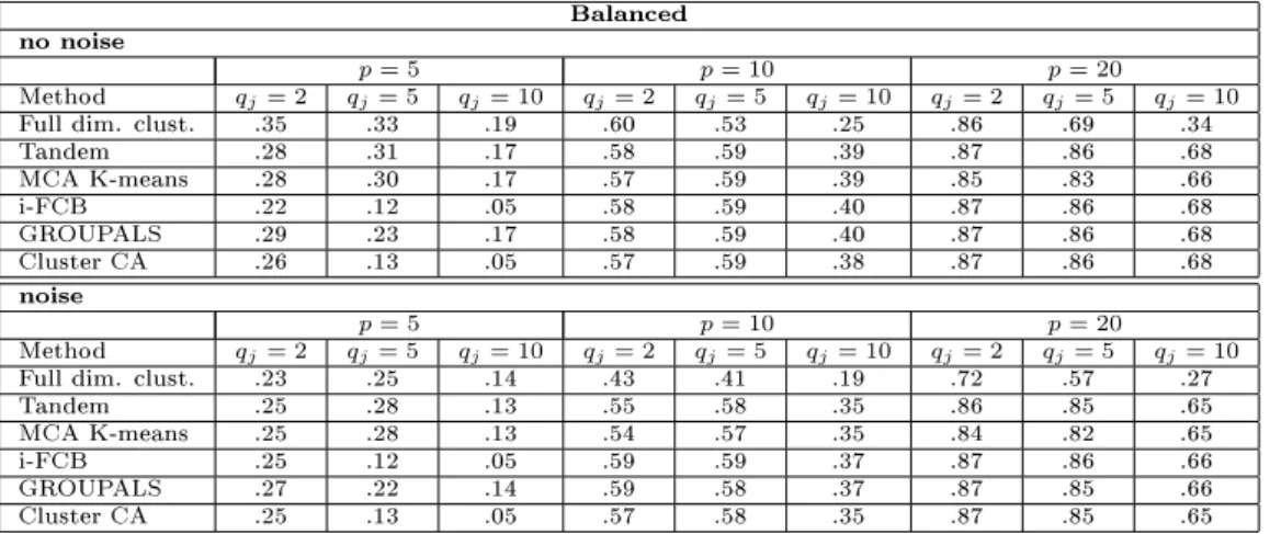
The cluster retrieval results for the balanced (i.e., the true clusters all have the same size) data can be found in Table 1. We see that by increasing the number of variables and categories, the joint dimension reduction and cluster analysis methods perform better than full dimensional clustering. Adding noise to the data amplies this result as the reduced dimension methods appear to be unaected by this. For few (5) variables, i-FCB and the new method have more diculty in retrieving the true clusters, however, when 10 or more variables are used, all methods perform similarly. The results for the unbalanced scenario, Table 2, are comparable. All methods have more diculty in retrieving the true clusters than in the balanced case. However, with the exception of i-FCB, which appears to suer more from the unbalancedness, the dierences are small.
Table 3 gives the results for mixed number of categories. We see that, the ARI values for the mixed cases are close to the average of the non-mixed scenarios.
The average silhouette values for the dierent scenarios are presented in Tables 4 through 6. We see that, in general, values are close to zero indicating not well separated clusters. The inuence of the number of categories on the average silhouette width is rather large and consistent for all methods, with few categories yielding much better results. Although adding noise did not appear to aect cluster allocation for the reduced dimension methods much, it does lead to a drop in the silhouette values for all methods. Apparently, individuals are correctly classied even though the clusters are less clearly separated.
Balanced no noise
p= 5 p= 10 p= 20
Method qj= 2 qj= 5 qj= 10 qj= 2 qj= 5 qj= 10 qj= 2 qj= 5 qj= 10
Full dim. clust. .35 .33 .19 .60 .53 .25 .86 .69 .34 Tandem .28 .31 .17 .58 .59 .39 .87 .86 .68 MCA K-means .28 .30 .17 .57 .59 .39 .85 .83 .66 i-FCB .22 .12 .05 .58 .59 .40 .87 .86 .68 GROUPALS .29 .23 .17 .58 .59 .40 .87 .86 .68 Cluster CA .26 .13 .05 .57 .59 .38 .87 .86 .68 noise p= 5 p= 10 p= 20 Method qj= 2 qj= 5 qj= 10 qj= 2 qj= 5 qj= 10 qj= 2 qj= 5 qj= 10
Full dim. clust. .23 .25 .14 .43 .41 .19 .72 .57 .27 Tandem .25 .28 .13 .55 .58 .35 .86 .85 .65 MCA K-means .25 .28 .13 .54 .57 .35 .84 .82 .65 i-FCB .25 .12 .05 .59 .59 .37 .87 .86 .66 GROUPALS .27 .22 .14 .59 .58 .37 .87 .85 .66 Cluster CA .25 .13 .05 .57 .58 .35 .87 .85 .65
Table 1: Average Adjusted Rand index (ARI) for simulated data using four equal sized clusters. The considered factors are: number of variables (5,10,20); number of categories per variable (2,5,10); presence/absence of noise variables.
Unbalanced no noise
p= 5 p= 10 p= 20
Method qj= 2 qj= 5 qj= 10 qj= 2 qj= 5 qj= 10 qj= 2 qj= 5 qj= 10
Full dim. clust. .34 .39 .27 .60 .48 .25 .89 .51 .28 Tandem .25 .26 .15 .48 .49 .28 .81 .82 .53 MCA K-means .25 .24 .15 .46 .45 .28 .74 .64 .47 i-FCB .19 .13 .04 .38 .37 .24 .59 .56 .40 GROUPALS .25 .18 .13 .46 .50 .29 .80 .82 .54 Cluster CA .24 .15 .06 .45 .47 .30 .78 .82 .52 noise p= 5 p= 10 p= 20 Method qj= 2 qj= 5 qj= 10 qj= 2 qj= 5 qj= 10 qj= 2 qj= 5 qj= 10
Full dim. clust. .21 .22 .20 .34 .34 .19 .50 .43 .21 Tandem .24 .23 .12 .44 .47 .25 .77 .79 .47 MCA K-means .23 .23 .12 .42 .44 .24 .72 .65 .44 i-FCB .20 .13 .04 .39 .36 .21 .56 .55 .37 GROUPALS .22 .19 .13 .44 .48 .25 .78 .80 .48 Cluster CA .21 .15 .06 .45 .48 .23 .77 .78 .45
Table 2: Average Adjusted Rand index (ARI) for simulated data using clusters with dierent sizes. The considered factors are: number of variables(5,10,20); number of categories per variable (2,5,10); presence/absence of noise variables.
5.5 Conclusions of the simulation study
The simulation study shows that dimension reduction improves clustering of high dimensional categorical data. There is no clear winner among the joint methods and the tandem approach also performs quite well. Note that, in our simulation study, the true dimensionality was not controlled for explicitly. Moreover, we did not consider scenarios involving so-called masking variables, that is, variables that "hide" cluster structure in the rst dimensions. For categorical data, it is not trivial how to generate such data in a fair and general way.
no noise
Balanced Unalanced
Method p= 5 p= 10 p= 20 p= 5 p= 10 p= 20
Full dim. clust. .29 .50 .69 .34 .50 .50
Tandem .25 .51 .81 .22 .41 .74 MCA K-means .25 .50 .81 .22 .39 .65 i-FCB .11 .52 .82 .13 .32 .52 GROUPALS .16 .52 .81 .13 .41 .74 Cluster CA .10 .50 .81 .12 .42 .72 noise Balanced Unalanced Method p= 5 p= 10 p= 20 p= 5 p= 10 p= 20
Full dim. clust. .22 .37 .55 .21 .30 .40
Tandem .23 .49 .80 .19 .37 .69
MCA K-means .22 .49 .79 .19 .36 .62
i-FCB .11 .51 .81 .10 .31 .51
GROUPALS .16 .50 .80 .14 .39 .70
Cluster CA .11 .49 .81 .12 .42 .69
Table 3: Average Adjusted Rand index (ARI) for simulated data. The considered factors are: balanced groups and unbalanced groups ; presence/absence of noise variables.; number of variables
(5,10,20)and a mixed distribution of categories per variable.
Balanced no noise
p= 5 p= 10 p= 20
Method pj= 2 pj= 5 pj= 10 pj= 2 pj= 5 pj= 10 pj= 2 pj= 5 pj= 10
Full dim. clust. .40 .14 .06 .29 .11 .04 .28 .10 .03 Tandem .39 .14 .06 .29 .12 .05 .28 .11 .04 MCA K-means .39 .14 .06 .29 .12 .05 .28 .11 .04 i-FCB .40 .20 .10 .29 .12 .05 .28 .11 .04 GROUPALS .41 .17 .07 .29 .12 .05 .28 .11 .04 Cluster CA .41 .20 .09 .29 .12 .05 .28 .11 .04 noise p= 5 p= 10 p= 20 Method pj= 2 pj= 5 pj= 10 pj= 2 pj= 5 pj= 10 pj= 2 pj= 5 pj= 10
Full dim. clust. .24 .08 .04 .17 .06 .02 .18 .06 .01 Tandem .25 .09 .04 .19 .08 .03 .20 .08 .03 MCA K-means .25 .09 .04 .19 .08 .03 .19 .07 .03 i-FCB .27 .14 .07 .20 .08 .03 .20 .08 .03 GROUPALS .27 .12 .05 .20 .08 .03 .20 .08 .03 Cluster CA .27 .14 .06 .20 .08 .03 .20 .08 .03
Table 4: Average silhouette index for simulated data using four equal sized clusters. The con-sidered factors are: number of variables (5,10,20); number of categories per variable (2,5,10);
Unbalanced no noise
p= 5 p= 10 p= 20
Method pj= 2 pj= 5 pj= 10 pj= 2 pj= 5 pj= 10 pj= 2 pj= 5 pj= 10
Full dim. clust. .43 .14 .06 .28 .09 .03 .28 .06 .02 Tandem .40 .13 .06 .27 .10 .04 .27 .11 .03 MCA K-means .40 .12 .06 .26 .10 .04 .24 .08 .03 i-FCB .40 .20 .10 .26 .10 .04 .21 .08 .03 GROUPALS .41 .18 .07 .27 .11 .04 .27 .11 .04 Cluster CA .42 .20 .09 .27 .11 .04 .26 .11 .04 noise p= 5 p= 10 p= 20 Method pj= 2 pj= 5 pj= 10 pj= 2 pj= 5 pj= 10 pj= 2 pj= 5 pj= 10
Full dim. clust. .25 .07 .04 .15 .05 .02 .12 .04 .01 Tandem .25 .09 .04 .17 .07 .03 .18 .07 .02 MCA K-means .25 .09 .04 .16 .07 .03 .16 .06 .02 i-FCB .27 .14 .07 .17 .07 .03 .14 .06 .02 GROUPALS .27 .12 .05 .18 .07 .03 .18 .07 .02 Cluster CA .28 .14 .07 .18 .08 .03 .18 .07 .02
Table 5: Average silhouette index for simulated data using clusters with dierent sizes. The considered factors are: number of variables(5,10,20); number of categories per variable(2,5,10);
presence/absence of noise variables.
no noise
Balanced Unalanced
Method p= 5 p= 10 p= 20 p= 5 p= 10 p= 20
Full dim. clust. .16 .11 .10 .18 .10 .06
Tandem .14 .11 .11 .14 .09 .10 MCA K-means .14 .10 .11 .14 .08 .09 i-FCB .21 .11 .11 .21 .09 .08 GROUPALS .17 .11 .11 .19 .09 .10 Cluster CA .19 .11 .11 .20 .10 .10 noise Balanced Unalanced Method p= 5 p= 10 p= 20 p= 5 p= 10 p= 20
Full dim. clust. .10 .07 .06 .11 .05 .04
Tandem .09 .07 .08 .09 .06 .07
MCA K-means .09 .07 .08 .09 .06 .06
i-FCB .15 .08 .08 .15 .06 .05
GROUPALS .12 .08 .08 .13 .06 .07
Cluster CA .14 .08 .08 .14 .07 .07
Table 6: Average silhouette index for simulated data. The considered factors are: balanced groups (top of the table) and unbalanced groups (bottom of the table); presence/absence of noise variables.; number of variables (5,10,20)and a mixed distribution of categories per variable.
6 Application
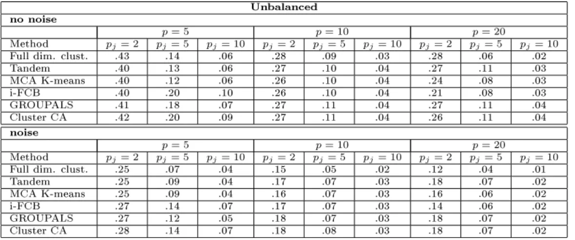
We apply our method to the results of a personality test, the Humor Styles Questionnaire, proposed by Martin et al. (2003). This questionnaire has been developed to measure four independent ways in which people express and appreciate humor: aliative, dened as the benign uses of humor to enhance one's relationships with others; self-enhancing, indicating uses of humor to enhance the self; aggressive, the use of humor to enhance the self at the expense of others; self-defeating the use of humor to enhance relationships at the expense of oneself. The questionnaire consists of 32 statements rated from 1 to 5 according to the respondents' level of agreement. The number of respondents is n= 993. The 32 statements and corresponding labels are reported in Table 7.
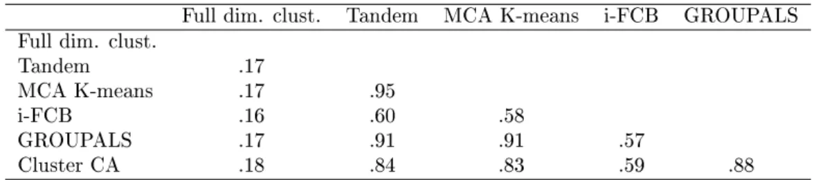
Martin et al. (2003) used the questionnaire to construct the humor styles. Here, we analyze the data from a dierent perspective: Can we distinguish clusters of individuals with similar humor proles? We apply the new cluster CA method to the data and use a two dimensional, three cluster solution. The solution depicting clusters and attributes is displayed in Figure 1. Using equation (12) we can project individual subject points into this CA map and thus visualize the variability within and between clusters. Figure 2 gives the corresponding map.
In CA, the origin depicts the average prole and all other points depict deviations from this average prole. The two dimensional displays, depicts two clearly separated clusters and one central cluster. To interpret the solution we consider individual attributes (i.e., a statement and category combination) and the positions of the cluster mean points relative to these. Note that, in cluster CA, the solotion for cluster means and category quantications constitute a biplot. Hence, these projections can be used to retrieve the observed values (see also Greenacre, 1993, on the biplot interpretation of correspondence analysis, in particular, on how to reconstruct the original data entries from a biplot).
From the two dimensional plot it is clear that cluster 1 appears to be associated with extreme categories (i.e., 1s or 5s) for the statements concerning self-defeating humor and self-enhancing humor. People in this group use humor to deal with bad situations (self-enhancing humor) and do so at their own expense. On the other side of the spectrum we nd a cluster of individuals (cluster 3 in Figure 1) indicating a preference for aliative humor. They show disagreement on statements concerning not laughing with others (and, agreement on "laughing with close friends"). The individuals in this cluster also indicate more than average disagreement concerning the statements regarding the use of humor to enhance the self. Furthermore, individuals in this cluster do not appreciate self-defeating humor. Finally, the cluster closest to the center of the plot (i.e., cluster
Label Statement Humor style Original question code AF1 I usually don't laugh or joke around much with other people. Aliative humor Q1
AF2 I don't have to work very hard at making other people laugh, Aliative humor Q5 I seem to be a naturally humorous person.
AF3 I rarely make other people laugh by telling funny stories about myself. Aliative humor Q9 AF4 I laugh and joke a lot with my closest friends. Aliative humor Q13 AF5 I usually don't like to tell jokes or amuse people. Aliative humor Q17 AF6 I enjoy making people laugh. Aliative humor Q21 AF7 I don't often joke around with my friends. Aliative humor Q25 AF8 I usually can't think of witty things to say when I'm with other people. Aliative humor Q29 SE1 If I am feeling depressed, I can usually cheer myself up with humor. Self-enhancing humor Q2 SE2 Even when I'm by myself, I'm often amused by the absurdities of life. Self-enhancing humor Q6 SE3 If I am feeling upset or unhappy, I usually try to think of something Self-enhancing humor Q10
funny about the situation to make myself feel better.
SE4 My humorous outlook on life keeps me from Self-enhancing humor Q14 getting overly upset or depressed about things.
SE5 If I'm by myself and I'm feeling unhappy, I make an eort to think of Self-enhancing humor Q18 something funny to cheer myself up.
SE6 If I am feeling sad or upset, I usually lose my sense of humor. Self-enhancing humor Q22 SE7 It is my experience that thinking about some amusing aspect Self-enhancing humor Q26
of a situation is often a very eective way of coping with problems.
SE8 I don't need to be with other people to feel amused Self-enhancing humor Q30 I can usually nd things to laugh about even when I'm by myself.
AG1 If someone makes a mistake, I will often tease them about it. Aggressive humor Q3 AG2 People are never oended or hurt by my sense of humor. Aggressive humor Q7 AG3 When telling jokes or saying funny things, I am usually not very Aggressive humor Q11
concerned about how other people are taking it.
AG4 I do not like it when people use humor as a way Aggressive humor Q15 of criticizing or putting someone down.
AG5 Sometimes I think of something that is so funny Aggressive humor Q19 that I can't stop myself from saying it,
even if it is not appropriate for the situation.
AG6 I never participate in laughing at others even if all my friends are doing it. Aggressive humor Q23 AG7 If I don't like someone, I often use humor or teasing to put them down. Aggressive humor Q27 AG8 Even if something is really funny to me, Aggressive humor Q31
I will not laugh or joke about it if someone will be oended.
SD1 I let people laugh at me or make fun at my expense more than I should. Self-defeating humor Q4 SD2 I will often get carried away in putting myself down Self-defeating humor Q8
if it makes my family or friends laugh.
SD3 I often try to make people like or accept me more by saying something Self-defeating humor Q12 funny about my own weaknesses, blunders, or faults.
SD4 I don't often say funny things to put myself down. Self-defeating humor Q16 SD5 I often go overboard in putting myself down when Self-defeating humor Q20
I am making jokes or trying to be funny.
SD6 When I am with friends or family, I often seem to be the one that Self-defeating humor Q24 other people make fun of or joke about.
SD7 If I am having problems or feeling unhappy, Self-defeating humor Q28 I often cover it up by joking around,
so that even my closest friends don't know how I really feel.
SD8 Letting others laugh at me is my way of keeping Self-defeating humor Q32 my friends and family in good spirits.
Table 7: Humor Styles Questionnaire: Each statement is rated from 1 (strongly disagree), to 5 (strongly agree); for each statement, the corresponding humor style and original question number is reported
2 in Figure 1) does not show extreme agreement/disagreement concerning any statement. People in this cluster exhibit preferences that are closely aligned with the average preferences. For these data this corresponds to agreement levels close to the center of the scale for most statements.
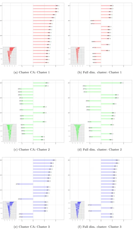
The interpretation given above is based on the visualization in Figure 1. To help with the inter-pretation of clusters it is useful to identify attributes that deviate the most from the independence condition. The three plots on the left side of Figure 3 (i.e. 3a, 3c, and 3e) show for each cluster the twenty attributes with the highest standardized residuals (positive or negative). A positive (negative) residual means that the attribute has an above (below) average frequency within the
cluster. Figure 3 clearly conrms the graphical depiction of Figure 1. We see that for cluster 1, agreement is high for the statements concerning the self-defeating and self-enhancing humor styles. (Note that some items indicate disagreement, however those items, for example SD4, are phrased reversely). Cluster 3 is characterized by respondents with an aliative humor style, as the group is mostly characterized by strong agreement on sentences (AF1, AF5, AF7, AF4, AF6, AF8), with AF1 and AF4 being on a reverse scale. This group also indicates disagreement with several of the self-defeating and self-enhancing humor styles. Finally, in cluster 2, respondents are less pronounced in their levels of agreement with the various humor styles. Instead, they tend to show medium levels of agreement on many attributes.
We compare the results of cluster CA with those of the other methods described in the paper. A true clustering is not known so we can only consider similarity of the low dimensional congu-rations and the dierent cluster partitions. Concerning the similarity of the congucongu-rations, Table 9 gives the congruency coecients (Borg & Groenen, 2005, pp. 437-440) between the attribute congurations. We see that the cluster CA solution is similar to the conguration obtained using GROUPALS. Also, similarity with the Tandem approach (i.e., the two dimensional MCA solution) is high. For these data, it appears that MCA K-means yields a less similar conguration.
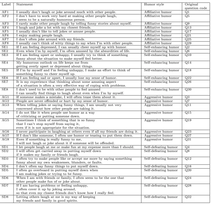
To compare the dierent cluster partitions we use the adjusted Rand index (ARI). We consider the results of all methods including full dimensional clustering where, as before in the simulation study, we use Gower dissimilarities and K-medoids clustering. The results are in Table 10. Again we see that the cluster CA solution is similar to the GROUPALS solution (.88), and, to a lesser
degree, the tandem and MCA K-means solutions (.84and.83, respectively). Both full dimensional
clustering and i-FCB yield rather dierent cluster partitions. Full dimensional clustering in partic-ular yields a solution that is quite dierent with ARI values around.18for all comparisons. These
dierences are also apparent when comparing the cluster size distributions in Table 8.
Similarity and dissimilarity of the methods with respect to each other does not indicate which method is better. However, based on the simulation study, the joint dimension methods are expected to perform better than the full dimensional clustering solution. This expectation is conrmed when considering the average silhouette width. Rounded to two decimals, this is for all dimension reduction and clustering methods.07whereas the value for full dimensional clustering
equals .03.
Such ndings are also evident from the two dimensional maps in Figure 1. In Figure 3, the 20 largest (in absolute value) standardized residuals per attribute are depicted for the three clusters obtained using cluster CA (the three gures on the left) and full dimensional clustering (the three
gures on the right). The clusters of the full dimensional solution have been ordered in such a way that they match the cluster size order of cluster CA. This side by side comparison, clearly illustrates that the clusters obtained using the new method are easier to interpret than those obtained using the full dimensional cluster results.
1 2 3 fullDim .27 .43 .30 Tandem .18 .45 .37 MCAk .18 .46 .36 iFCB .27 .38 .35 Groupals .18 .45 .37 CAclus .18 .43 .39
Table 8: Relative cluster size distributions: clusters are ordered to match the Cluster CA solution order
Tandem MCA K-means i-FCB GROUPALS Tandem
MCA K-means .78
i-FCB .95 .77
GROUPALS .97 .79 .95
Cluster CA .86 .68 .90 .90
Table 9: Two-by-two congruency index of the low-dimensional attribute congurations as produced by the methods
Full dim. clust. Tandem MCA K-means i-FCB GROUPALS Full dim. clust.
Tandem .17
MCA K-means .17 .95
i-FCB .16 .60 .58
GROUPALS .17 .91 .91 .57
Cluster CA .18 .84 .83 .59 .88
Table 10: Adjusted Rand indices between the dierent partitions
7 Conclusions
This paper proposes a new method that combines cluster analysis and correspondence analysis. The new method can be seen as correspondence analysis of a cluster by variable association table and yields, in addition to a low-dimensional approximation depicting clusters and attributes, a cluster partitioning of individuals based on the proles over the categorical variables. We showed how the new method relates to existing methods for joint dimension reduction and clustering of categorical data. Using a simulation study, we assessed the performances of the methods. Upon the
AF1: 1 AF1: 2 AF1: 3 AF1: 4 AF1: 5 SE1: 1 SE1: 2 SE1: 3 SE1: 4 SE1: 5 AG1: 1 AG1: 2 AG1: 3 AG1: 4 AG1: 5 SD1: 1 SD1: 2 SD1: 3 SD1: 4 SD1: 5 AF2: 1 AF2: 2 AF2: 3 AF2: 4 AF2: 5 SE2: 1 SE2: 2 SE2: 3 SE2: 4 SE2: 5 AG2: 1 AG2: 2 AG2: 3 AG2: 4 AG2: 5 SD2: 1 SD2: 2 SD2: 3 SD2: 4 SD2: 5 AF3: 1 AF3: 2 AF3: 3 AF3: 4 AF3: 5 SE3: 1 SE3: 2 SE3: 3 SE3: 4 SE3: 5 AG3: 1 AG3: 2 AG3: 3 AG3: 4 AG3: 5 SD3: 1 SD3: 2 SD3: 3 SD3: 4 SD3: 5 AF4: 1 AF4: 2 AF4: 3 AF4: 4 AF4: 5 SE4: 1 SE4: 2 SE4: 3 SE4: 4 SE4: 5 AG4: 1 AG4: 2 AG4: 3 AG4: 4 AG4: 5 SD4: 1 SD4: 2 SD4: 3 SD4: 4 SD4: 5 AF5: 1 AF5: 2 AF5: 3 AF5: 4 AF5: 5 SE5: 1 SE5: 2 SE5: 3 SE5: 4 SE5: 5 AG5: 1 AG5: 2 AG5: 3 AG5: 4 AG5: 5 SD5: 1 SD5: 2 SD5: 3 SD5: 4 SD5: 5 AF6: 1 AF6: 2 AF6: 3 AF6: 4 AF6: 5 SE6: 1 SE6: 2 SE6: 3 SE6: 4 SE6: 5 AG6: 1 AG6: 2 AG6: 3 AG6: 4 AG6: 5 SD6: 1 SD6: 2 SD6: 3 SD6: 4 SD6: 5 AF7: 1 AF7: 2 AF7: 3 AF7: 4 AF7: 5 SE7: 1 SE7: 2 SE7: 3 SE7: 4 SE7: 5 AG7: 1 AG7: 2 AG7: 3 AG7: 4 AG7: 5 SD7: 1 SD7: 2 SD7: 3 SD7: 4 SD7: 5 AF8: 1 AF8: 2 AF8: 3 AF8: 4 AF8: 5 SE8: 1 SE8: 2 SE8: 3 SE8: 4 SE8: 5 AG8: 1 AG8: 2 AG8: 3 AG8: 4 AG8: 5 SD8: 1 SD8: 2 SD8: 3 SD8: 4 SD8: 5 C1 C2 C3
Figure 1: Cluster Correspondence analysis biplot. Scaling as dened in equation (14). Attribute labels correspond to the labels in Table 7 with category numbers added. Cluster means are labelled C1 through C3.
results of our simulation study we can state that categorical data clustering benets from dimension reduction. That is, with respect to retrieval of true underlying cluster structure, joint dimension reduction and clustering methods outperform full dimensional clustering for high dimensional.
Among the joint dimension reduction and clustering methods, dierences were relatively small both with respect to cluster retrieval and internal cluster validity. This is not surprising because data coding and centering were the same for all the considered methods. However, there are some important points in favor of the new method. First, when cluster sizes are not equal, the i-FCB method has an higher failure rate than the other methods. Secondly, although it is possible in MCA K-means to obtain and plot individual subject points, the coordinates of these subject points are not insightful as they are inuenced by the (user selected) weights assigned to the MCA and K-means part of the objective. With respect to these weights it should be noted that, in this paper, we only considered equal weights. It is not clear which criteria to use to tune this parameter but results are dependent on that choice.
AF1: 1 AF1: 2 AF1: 3 AF1: 4 AF1: 5 SE1: 1 SE1: 2 SE1: 3 SE1: 4 SE1: 5 AG1: 1 AG1: 2 AG1: 3 AG1: 4 AG1: 5 SD1: 1 SD1: 2 SD1: 3 SD1: 4 SD1: 5 AF2: 1 AF2: 2 AF2: 3 AF2: 4 AF2: 5 SE2: 1 SE2: 2 SE2: 3 SE2: 4 SE2: 5 AG2: 1 AG2: 2 AG2: 3 AG2: 4 AG2: 5 SD2: 1 SD2: 2 SD2: 3 SD2: 4 SD2: 5 AF3: 1 AF3: 2 AF3: 3 AF3: 4 AF3: 5 SE3: 1 SE3: 2 SE3: 3 SE3: 4 SE3: 5 AG3: 1 AG3: 2 AG3: 3 AG3: 4 AG3: 5 SD3: 1 SD3: 2 SD3: 3 SD3: 4 SD3: 5 AF4: 1 AF4: 2 AF4: 3 AF4: 4 AF4: 5 SE4: 1 SE4: 2 SE4: 3 SE4: 4 SE4: 5 AG4: 1 AG4: 2 AG4: 3 AG4: 4 AG4: 5 SD4: 1 SD4: 2 SD4: 3 SD4: 4 SD4: 5 AF5: 1 AF5: 2 AF5: 3 AF5: 4 AF5: 5 SE5: 1 SE5: 2 SE5: 3 SE5: 4 SE5: 5 AG5: 1 AG5: 2 AG5: 3 AG5: 4 AG5: 5 SD5: 1 SD5: 2 SD5: 3 SD5: 4 SD5: 5 AF6: 1 AF6: 2 AF6: 3 AF6: 4 AF6: 5 SE6: 1 SE6: 2 SE6: 3 SE6: 4 SE6: 5 AG6: 1 AG6: 2 AG6: 3 AG6: 4 AG6: 5 SD6: 1 SD6: 2 SD6: 3 SD6: 4 SD6: 5 AF7: 1 AF7: 2 AF7: 3 AF7: 4 AF7: 5 SE7: 1 SE7: 2 SE7: 3 SE7: 4 SE7: 5 AG7: 1 AG7: 2 AG7: 3 AG7: 4 AG7: 5 SD7: 1 SD7: 2 SD7: 3 SD7: 4 SD7: 5 AF8: 1 AF8: 2 AF8: 3 AF8: 4 AF8: 5 SE8: 1 SE8: 2 SE8: 3 SE8: 4 SE8: 5 AG8: 1 AG8: 2 AG8: 3 AG8: 4 AG8: 5 SD8: 1 SD8: 2 SD8: 3 SD8: 4 SD8: 5 C1 C2 C3
Figure 2: Cluster Correspondence analysis biplot with projected subject points. Scaling as dened in equation (14). Attribute labels correspond to the labels in Table 7 with category numbers added. Cluster 1 points are represented by `+', cluster 2 points by `◦' and cluster 3 points by `4'.
in which clustering is performed after dimension reduction, could be problematic. In our simulation study, we did not nd evidence for this in the categorical variable case. Unlike the simulation study designed by Vichi & Kiers (2001), we did not consider scenarios in which so-called masking variables were used to hide cluster structure in the reduced space. It could be the case that scenarios can be constructed were the tandem approach does suer from the sequential analysis.
Our simulation clearly demonstrated that for high dimensional categorical data dimension re-duction improves the clustering results. In presence of noise variables (i.e., variables unrelated to the cluster structure) the dierence increased. Possible reasons for this failure of full dimensional clustering versus joint dimension reduction approaches, are the fact that the true dimensionality of the data is typically not equal to the size of the data table and that the exaggerated dimensionality of the data table contains noise that is ltered out in the joint dimension reduction methods.
SE3: 1 SE7: 1 SE4: 1 SE5: 1 SD8: 1 SD7: 1 AF2: 1 AF3: 5 AF6: 2 AG5: 1 SD2: 1 SE1: 1 AG1: 1 AF5: 5 SD1: 1 SD4: 5 SE1: 2 SE6: 5 SD3: 1 AF2: 2 5 10 15 20 −2 −1 0 1 2 0 50 100 150 −2−1 0 1 2
(a) Cluster CA: Cluster 1
AF8: 2 SE4: 4 AF2: 4 SE7: 4 SE6: 2 AG4: 5 SD7: 1 SE2: 4 SE8: 4 SE5: 3 AG8: 2 AG7: 3 SD4: 5 SD2: 2 AF7: 2 AG5: 4 SD2: 1 AG2: 5 AG3: 1 SD1: 1 5 10 15 20 −2 −1 0 1 2 0 50 100 150 −2−1 0 1 2
(b) Full dim. cluster: Cluster 1 AF5: 2 AF7: 2 AF5: 1 SE4: 5 AF8: 1 AF1: 1 AF2: 5 AG8: 1 AF1: 2 AF3: 1 AF4: 4 AG3: 5 AG5: 5 AF6: 4 SE2: 5 AG1: 5 SD4: 1 SE8: 5 SE2: 4 SD5: 2 5 10 15 20 −2 −1 0 1 2 0 50 100 150 −2−1 0 1 2
(c) Cluster CA: Cluster 2
AF7: 2 AF5: 1 AF7: 1 AF1: 1 AF4: 4 AF6: 4 AF6: 5 SE2: 3 AF4: 5 AF8: 1 SE5: 2 AF5: 2 AF8: 3 AF2: 5 AF2: 3 SE4: 5 AF3: 1 AG5: 2 SD5: 1 SE3: 2 5 10 15 20 −2 −1 0 1 2 0 50 100 150 −2−1 0 1 2
(d) Full dim. cluster: Cluster 2 AF5: 1 SE4: 5 AF1: 1 AF2: 5 AF8: 1 AF3: 1 SE2: 5 AG5: 5 AF7: 2 SE7: 5 AF7: 1 AF6: 5 AF4: 5 AF4: 4 AG1: 5 AG8: 1 SD7: 5 SE8: 5 AF5: 2 AF6: 4 5 10 15 20 −2 −1 0 1 2 0 50 100 150 −2−1 0 1 2
(e) Cluster CA: Cluster 3
SD4: 5 AF8: 1 AF2: 5 SE4: 5 SD2: 1 SD8: 1 SE7: 5 SE2: 5 AG5: 5 SD6: 1 SD1: 1 SE8: 5 AG2: 5 AF3: 1 AG3: 5 AF7: 2 SD7: 1 AF5: 2 SD5: 1 SD3: 1 5 10 15 20 −2 −1 0 1 2 0 50 100 150 −2−1 0 1 2
(f) Full dim. cluster: Cluster 3
Figure 3: Top 20's of the largest standardized residuals per cluster (with complete distributions in small subplots) for Cluster CA (left) and full dimensional clustering (right)
References
Borg, I., & Groenen, P. J. (2005). Modern multidimensional scaling: Theory and applications. Springer.
De Soete, G., & Carroll, J. D. (1994). K-means clustering in a low-dimensional euclidean space. In E. Diday, Y. Lechevallier, M. Schader, P. Bertrand, & B. Burtschy (Eds.), New approaches in classication and data analysis (p. 212-219). Springer-Verlag, Berlin.
Gower, J. C. (1971). A general coecient of similarity and some of its properties. Biometrics, 27 , 623-637.
Gower, J. C., Gardner Lubbe, S., & Le Roux, N. J. (2011). Understanding biplots. John Wiley & Sons.
Gower, J. C., Groenen, P. J. F., & van de Velden, M. (2010). Area biplots. Journal of Computa-tional and Graphical Statistics, 19 (1), 46-61.
Gower, J. C., & Hand, D. J. (1996). Biplots. London: Chapman and Hall.
Greenacre, M. J. (1984). Theory and applications of correspondence analysis. London: Academic Press.
Greenacre, M. J. (1993). Biplots in correspondence analysis. Journal of Applied Statistics, 20 (2), 251269.
Hubert, L., & Arabie, P. (1985). Comparing partitions. Journal of Classication, 2 (1), 193-218. Retrieved from http://dx.doi.org/10.1007/BF01908075 doi: 10.1007/BF01908075
Hwang, H., Dillon, W. R., & Takane, Y. (2006). An extension of multiple correspondence analysis for identifying heterogenous subgroups of respondents. Psychometrika, 71 , 161-171.
Iodice D'Enza, A., & Palumbo, F. (2013). Iterative factor clustering of binary data. Computa-tional Statistics, 789-807. Retrieved from http://dx.doi.org/10.1007/s00180-012-0329-x (10.1007/s00180-012-0329-x)
Iodice D'Enza, A., van de Velden, M., & Palumbo, F. (2014). On joint dimension reduction and clustering of categorical data. In D. Vicari, A. Okada, G. Ragozini, & C. Weihs (Eds.), Analysis and modeling of complex data in behavioral and social sciences. Springer, Berlin.
Kroonenberg, P. M., & Lombardo, R. (1999). Nonsymmetric correspondence analysis: a tool for analysing contingency tables with a dependence structure. Multivariate Behavioral Research, 34 , 367396.
Lauro, N., & D'Ambra, L. (1984). L' analyse non symetrique des correspondances [nonsymmetric correspondence analysis]. In E. Diday, L. Lebart, M. Jambu, & Thomassone (Eds.), Data analysis and informatics iii (p. 433-446). Elsevier, Amsterdam.
Martin, R. A., Puhlik-Doris, P., Larsen, G., Gray, J., & Weir, K. (2003). Individual dierences in uses of humor and their relation to psychological well-being: Development of the humor styles questionnaire. Journal of research in personality, 37 (1), 4875.
Nishisato, S. (1980). Analysis of categorical data: dual scaling and its applications. Toronto: University of Toronto Press.
Nishisato, S. (1994). Elements of dual scaling: an introduction to practical data analysis. Hillsdale, New Jersey: Lawrence Erlbaum Associates.
Rousseeuw, P. J. (1987). Silhouettes: A graphical aid to the interpretation and validation of cluster analysis. Journal of Computational and Applied Mathematics, 20 (0), 53 - 65. Retrieved from http://www.sciencedirect.com/science/article/pii/0377042787901257 doi: http://dx .doi.org/10.1016/0377-0427(87)90125-7
van de Velden, M., & Bijmolt, T. (2006). Generalized canonical correlation analysis of matrices with missing rows: a simulation study. Psychometrika, 71 (2), 323-331.
van de Velden, M., & Takane, Y. (2012). Generalized canonical correlation analysis with missing values. Computational Statistics, 27 (3), 551-571.
Van Buuren, S., & Heiser, W. (1989). Clustering n objects into k groups under optimal scaling of variables. Psychometrika, 54 , 699-706.
Vichi, M., & Kiers, H. A. L. (2001). Factorial k-means analysis for two-way data. Computational Statistics and Data Analysis, 37 , 49-64.
Vichi, M., Vicari, D., & Kiers, H. (2009). Clustering and dimensional reduction for mixed variables. (Unpublished manuscript)
Yamamoto, M., & Hwang, H. (2014). A general formulation of cluster analysis with dimension reduction and subspace separation. Behaviormetrika, 41 , 115-129.