2014
Fractional imputation method of handling missing
data and spatial statistics
Shu Yang
Iowa State University
Follow this and additional works at:https://lib.dr.iastate.edu/etd Part of theStatistics and Probability Commons
This Dissertation is brought to you for free and open access by the Iowa State University Capstones, Theses and Dissertations at Iowa State University Digital Repository. It has been accepted for inclusion in Graduate Theses and Dissertations by an authorized administrator of Iowa State University Digital Repository. For more information, please [email protected].
Recommended Citation
Yang, Shu, "Fractional imputation method of handling missing data and spatial statistics" (2014).Graduate Theses and Dissertations. 13802.
by
Shu Yang
A dissertation submitted to the graduate faculty in partial fulfillment of the requirements for the degree of
DOCTOR OF PHILOSOPHY
Co-majors: Applied Mathematics; Statistics
Program of Study Committee: Alexander Roitershtein, Co-major Professor
Jae Kwang Kim, Co-major Professor Zhengyuan Zhu, Co-major Professor
Arka P. Ghosh Douglas Nychka
Sarah Nusser
Iowa State University Ames, Iowa
2014
TABLE OF CONTENTS
ABSTRACT . . . vi
CHAPTER 1. OVERVIEW . . . 1
CHAPTER 2. PARAMETRIC FRACTIONAL IMPUTATION FOR MIXED MOD-ELS WITH NONIGNORABLE MISSING DATA . . . 4
2.1 Introduction . . . 5
2.2 Linear mixed model with nonignorable missing values . . . 7
2.2.1 Basic setup . . . 7
2.2.2 Parametric fractional imputation maximum likelihood estimation . . 10
2.3 Adjusted profile likelihood for bias correction . . . 13
2.4 Simulation study of linear mixed model with nonignorable missing data . . . 15
2.5 Generalized linear mixed model . . . 18
2.5.1 Data description . . . 18
2.5.2 Generalized linear mixed model . . . 19
2.5.3 Fractional Imputation . . . 20
2.6 Discussion Remark . . . 22
2.7 Appendix section - Variance estimation . . . 22
CHAPTER 3. IMPUTATION METHODS FOR QUANTILE ESTIMATION UN-DER MISSING AT RANDOM . . . 27
3.1 Introduction . . . 27
3.2.1 Multiple Imputation (MI) . . . 30
3.2.2 Parametric Fractional Imputation (PFI) . . . 31
3.3 Proposed methods . . . 33
3.3.1 Fractional hot deck imputation (FHDI) . . . 33
3.3.2 Nonparametric fractional imputation (NPFI) . . . 34
3.4 Variance estimation . . . 35
3.5 Simulation Study . . . 37
3.5.1 Simulation . . . 38
3.5.2 Real Data Analysis . . . 41
3.6 Concluding remarks . . . 42
3.7 Appendix section . . . 43
3.7.1 Variance estimation in PFI . . . 43
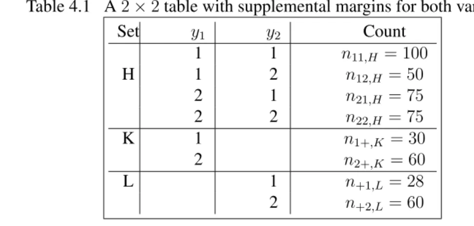
CHAPTER 4. LIKELIHOOD-BASED INFERENCE WITH MISSING DATA UN-DER MISSING-AT-RANDOM . . . 52 4.1 Introduction . . . 53 4.2 Basic setup . . . 54 4.3 Proposed method . . . 56 4.4 Computation details . . . 66 4.5 Simulation Study . . . 68
4.5.1 Profile likelihood confidence interval . . . 68
4.5.2 Likelihood ratio test . . . 69
4.6 Real data example . . . 71
4.7 Discussion . . . 73
CHAPTER 5. A SEMIPARAMETRIC INFERENCE TO REGRESSION ANAL-YSIS WITH MISSING COVARIATES IN SURVEY DATA . . . 92
5.1 Introduction . . . 93
5.3 Main theoretical results . . . 95
5.4 Computation . . . 97
5.5 Extensions to general parameter estimation . . . 99
5.6 Simulation study . . . 101
5.6.1 Simulation one - Linear model . . . 101
5.6.2 Simulation two - Poisson regression model . . . 105
5.7 Concluding remarks . . . 108
CHAPTER 6. VARIANCE ESTIMATION AND KRIGING PREDICTION FOR A CLASS OF NON-STATIONARY SPATIAL MODELS . . . 118
6.1 Introduction . . . 118
6.2 Methodology . . . 121
6.2.1 Difference-based kernel estimator . . . 121
6.2.2 Modified likelihood estimator ofσ2 . . . 123
6.2.3 Bandwidth selection . . . 124
6.2.4 Kriging prediction . . . 125
6.3 Theoretical Results . . . 126
6.4 Simulation studies . . . 130
6.4.1 Simulation One - Variance estimation . . . 130
6.4.2 Simulation Two - Kriging versus spatially adaptive local polynomial fitting . . . 131
6.5 Discussions . . . 133
6.6 Supplementary Materials . . . 134
6.7 References . . . 144
CHAPTER 7. SEMIPARAMETRIC ESTIMATION OF SPECTRAL DENSITY FUNCTION FOR IRREGULAR SPATIAL DATA . . . 149
7.1 Introduction . . . 150
7.2.1 Smoothing spline estimation of spectral density at low frequencies . . 154
7.2.2 Estimation of the decay rate . . . 155
7.2.3 Adjusting for Aliasing and the final spectral density estimator . . . . 157
7.3 Asymptotic Results . . . 158 7.4 Simulation study . . . 161 7.4.1 Simulation setup . . . 161 7.4.2 Estimation . . . 161 7.4.3 Spatial kriging . . . 162 7.5 Discussion Remarks . . . 166
ABSTRACT
This thesis has two themes. One is missing data analysis, and the other is spatial data analysis.
Missing data frequently occur in many statistics problems. It can arise naturally in many applications. For example, in many surveys there are data that could have been observed are missing due to non-response. It can also be a deliberate modeling choice. For example, a mixed effects model can include random variables that are not observable (called latent variables or random effects). Imputation is often used to facilitate parameter estimation in the presence of missing data, which allows one to use the complete sample estimators on the imputed data set. Parametric fractional imputation (PFI) is an imputation method proposed by Kim (2011), which simplifies the computation associated with the EM algorithm for maximum likelihood estimation with missing data. In this thesis we study four extensions of the PFI methods: 1. The use of PFI to handle non-ignorable non-response problem in linear and generalized linear mixed models. 2. Application of PFI method for quantile estimation with missing data. 3. Likelihood-based inference for missing data using PFI. 4. A semiparametric fractional imputation method for handling missing covariate.
The second theme is spatial data analysis. Estimation of the covariance structure of spa-tial processes is of fundamental importance in spaspa-tial statistics. The difficulty arises when spatial process exhibits non-stationarity or the observed spatial data is irregularly spaced. We propose estimation methods targeting to solve these two difficulties. 1. We propose a non-stationary spatial modeling, study the theoretical properties of estimation and plug-in kriging prediction of a non-stationary spatial process, and explore the connection between kriging un-der non-stationary models and spatially adaptive non-parametric smoothing methods. 2. A
CHAPTER 1. OVERVIEW
Inference in the presence of missing data is a widely encountered and difficult problem in statistics. Imputation is often used to facilitate parameter estimation, which allows one to use the complete sample estimators on the imputed data set. In Chapter2, We develop a parametric fractional imputation (PFI) method proposed by Kim (2011), which simplifies the computation associated with the EM algorithm for maximum likelihood estimation with missing data. We first consider the problem of parameter estimation for linear mixed models with non-ignorable missing values, which assumes that missingness depends on the missing values only through the random effects, leading to shared parameter models (Follmann and Wu,1995). In the M-step, the restricted or adjusted profiled maximum likelihood method is used to reduce the bias of maximum likelihood estimation of the variance components. Results from a limited simulation study are presented to compare the proposed method with the existing methods, which demonstrates that imputation can significantly reduce the non-response bias and the idea of adjusted profiled maximum likelihood works nicely in PFI for the bias correction in estimating the variance components. Variance estimation is also discussed. We next extend PFI to generalized linear mixed model and the flexibility of this method is illustrated by analyzing the infamous salamander mating data (McCullagh and Nelder, 1989).
In Chapter3, we propose a fractional hot deck imputation which produces a valid variance estimator for quantiles. In the proposed method, the imputed values are chosen from the set of responses and are assigned with proper fractional weights that use a density function for the working model. In addition, we consider a nonparametric fractional imputation method based on nonparametric kernel regression method, avoiding a parametric distribution assumption and
thus giving more robustness. The resulting estimator can be called nonparametric fractionally imputation estimator. Valid variance estimation is also discussed. A limited simulation study compares the proposed methods favorably compared with other existing methods.
Chapter 5 is devoted to parameter estimation in parametric regression models with co-variates missing at random in survey data. A semiparametric maximum likelihood approach is proposed which requires no parametric specification of the marginal covariate distribution. We obtain an asymptotic linear representation of the semiparametric maximum likelihood estima-tor (SMLE) using the theory of von Mises calculus and V Statistics, which allows a consistent estimator of asymptotic variance. An EM-type algorithm for computation is discussed. We extend the methodology for general parameter estimation, which is not necessary confined to MLE. Simulation results suggest that the SMLE method is robust, whereas the parametric maximum likelihood method is subject to severe bias under model misspecification.
Chapter 6 is devoted to another theme which is the modeling of non-stationary spatial data. We study the theoretical properties of estimation and plug-in kriging prediction of a non-stationary spatial process. We assume the process has smoothly varying variance function with an additive independent measurement error to account for the heterosexuality in the data. A difference-based kernel estimators of the variance function and a modified likelihood estimator of the measurement variance are proposed for parameter estimation. Asymptotic properties of these estimators and the plug-in kriging predictor are established. Simulation studies are pre-sented to test our estimation-prediction procedure and the performance of krigging predictor is compared with the spatial adaptive local polynomial regression estimator proposed by Fan and Gijbels (1995).
Chapter7is devoted to estimation of the covariance structure of spatial processes in spatial statistics. In the literature, several nonparametric and semi-parametric methods has been de-veloped to estimate the covariance structure based on the spectral representation of covariance functions. However, they either ignore the high frequency properties of the spectral density, which is essential to determine the performance of interpolation procedures such as kriging,
or lack theoretical justifications. We propose a new semi-parametric method to estimate spec-tral densities of isotropic Gaussian processes with irregular observations. The specspec-tral density function at low frequencies is estimated using smoothing spline, while a parametric model is used for the spectral density at high frequencies and the parameters estimated using method-of-moment based on empirical variogram at small lags. We derive the asymptotic bounds for bias and variance of the proposed estimator, and simulation results show that our method outperforms the existing nonparametric estimator by several performance criteria.
CHAPTER 2. PARAMETRIC FRACTIONAL IMPUTATION FOR
MIXED MODELS WITH NONIGNORABLE MISSING DATA
A paper is published inStatistics and Its Interface1
Shu Yang2, Jae Kwang Kim3, and Zhengyuan Zhu4
Abstract
Inference in the presence of non-ignorable missing data is a widely encountered and dif-ficult problem in statistics. Imputation is often used to facilitate parameter estimation, which allows one to use the complete sample estimators on the imputed data set. We develop a parametric fractional imputation (PFI) method proposed by Kim (2011), which simplifies the computation associated with the EM algorithm for maximum likelihood estimation with miss-ing data. We first consider the problem of parameter estimation for linear mixed models with non-ignorable missing values, which assumes that missingness depends on the missing values only through the random effects, leading to shared parameter models (Follmann and Wu,1995). In the M-step, the restricted or adjusted profiled maximum likelihood method is used to reduce the bias of maximum likelihood estimation of the variance components. Results from a lim-ited simulation study are presented to compare the proposed method with the existing methods, which demonstrates that imputation can significantly reduce the non-response bias and the idea of adjusted profiled maximum likelihood works nicely in PFI for the bias correction in
esti-1Reprinted with permission of Statistics and Its Interface,2013,6, 339–347. 2Primary researcher and author.
3Author for correspondence. 4Author for correspondence.
mating the variance components. Variance estimation is also discussed. We next extend PFI to generalized linear mixed model and the flexibility of this method is illustrated by analyzing the infamous salamander mating data (McCullagh and Nelder, 1989).
2.1
Introduction
Mixed models are the statistical models containing both fixed effects and random effects. These models are particularly useful in settings where repeated measurements are made on the same statistical units, or where measurements are made on the clustered elements.
However, missing data frequently occurs in mixed models and destroys the representative-ness of the remaining sample. There are several assumptions about the missing mechanism. If the missing probability is unrelated to the missing value after adjusting for the observed auxiliary information, the missing mechanism is called missing at random (MAR) or ignor-able; whereas if the missing probability is related to the missing value even after adjusting for the auxiliary information, the missing mechanism is called missing not at random (MNAR) or nonignorable. To model the nonignorable missing mechanism we considered the selec-tion model (Diggle and Kenward, 1994) approach. Specially, we consider a special case of the selection model, where missingness depends only on the random effects, which yields the so-called shared parameter models, considered by Wu and Carroll (1988), Follmann and Wu (1995) and Ten Have et al. (1998). Wu and Carroll (1988) considered a linear mixed effects model and a discrete-time survival model for the drop-out process that share a random effect structure. Follmann and Wu (1995) considered a conditional model to approximate the shared parameter binary response model conditional on missing data patterns. Ten Have et al. (1998) proposed mixed effects logistic regression models for longitudinal binary response data with informative drop-out.
To carry out the likelihood-based inference under the nonignorable missing, we may need to obtain the marginal density of the observed data, which involves integrating out the missing
part of the data. Except for a few special cases this is analytically infeasible and thus requires numerical integration. Usually, the marginal likelihood involves a high dimensional integral and numerical integration may not be feasible or reliable. One solution to this problem is im-putation. By imputation, one can construct a complete data set by assigning reasonable values for the missing data. It has several advantages. First, it facilitates the parameter estimation by simply applying the complete-sample estimators to the imputed data set. Second, it ensures different analyses are consistent with one another. Also, proper choice of imputation method often reduces the non-response bias.
Integration approximated by imputation under nonignorable missing was considered by many authors, Greenlees et al. (1982) considered the normal-theory linear regression model using a version of EM algorithm. Ibrahim et al. (1999) considered continuous variable using a Monte Carlo EM method of Wei and Tanner (1990) to compute the E-step of the EM algorithm in a generalized linear mixed model. Booth and Hobert (1999) used an automated Monte Carlo EM algorithm to compute the E-step of the EM algorithm to speed up the convergence rate. Chan and Kuk (1997) applied Gibbs sampling in the E-step to obtain maximum likelihood estimates for the probit normal model for binary data. McCulloch (1997) proposed a Monte Carlo Newton-Raphson algorithm in the maximum likelihood algorithm for generalized linear mixed models. For Monte Carlo EM algorithm, in each E-step, the imputed values are regen-erated and thus the computation can be quite heavy. Also the convergence of Monte Carlo sequence of the estimators is not guaranteed for fixed Monte Carlo sample size (Booth and Hobert, 1999).
In this paper, we develop a parametric fractional imputation (PFI) method proposed by Kim (2011) which can be used to simplify the Monte Carlo implementation of the EM algorithm, for linear mixed models with the shared parameter response model and for the generalized linear mixed model. The main idea in PFI is to produce a complete data set by imputation and each imputed value is associated with a fractional weight, by which the observed likelihood can be approximated by the weighted average of the imputed data likelihood. The resulting estimator
is close to the maximum likelihood estimator and has very nice asymptotic properties, such as efficiency and asymptotic normality.
PFI can also be extended to generalized linear mixed model. The flexibility of this method is illustrated by analyzing the infamous salamander mating data (McCullagh and Nelder, 1989). The data is challenging since the response variable is binary and the experimental design is crossed which causes serious limitations due to the intensive computations to ap-proximate the intractable joint distribution.
In Section 2, we introduce linear mixed model with nonignorable missing and develop the PFI method for this model. In Section 3, we discuss incorporation of adjusted profile likelihood estimation in PFI to reduce the bias in estimating variance components. In Section 4, results from a limited simulation study is presented. Section 5 demonstrates PFI in a generalized linear mixed model setting by analyzing the salamander mating data. We conclude with discussion in Section 6.
2.2
Linear mixed model with nonignorable missing values
2.2.1 Basic setup
In this section we introduce the data model and the missing mechanism model considered in the paper. We consider the linear mixed model
yij =β0+β1xij +bi+eij,i= 1, . . . , n, j = 1, . . . , m, (2.1)
where i indexes individual, j indexes the repeated measurement within each individual, bi
are i.i.d. from N(0, τ2) specifying the unobserved individual effects and e
ij are i.i.d. from
N(0, σ2), which are the measurement errors within individuals.
Letyi = (yi1, . . . , yim)0be the complete measurements on theithindividual if they are fully
observed. The observed and missing components are denoted asyobs,i,ymis,i respectively, so yi = (yobs,i,ymis,i). Let ri = (ri1, . . . , rim)0 be vector of indicators of response status, so
rij = 1 if yij is observed, otherwise, rij = 0.As a motivating example, consider a disease
longitudinal study. When patients experience an increase in pain, they might decide not to show up at some of the scheduled visits for disease evaluation. In the above cases, if we simply ignore the missingness process and use the standard procedure to analyze the data, the inference will be seriously biased. To take care of such an informative nonresponse, joint modeling of disease measurement and missing process is necessary.
To model the missing mechanism, we consider the selection model
f(yi,ri, bi) =f(yi|bi)f(ri|yi, bi)f(bi). (2.2)
Furthermore, in the selection model, we assume that nonignorable dropout in longitudinal data (Molenberghs and Kenward, 2009) where missingness depends on the missing values only through the random effectsf(ri|yi, bi) = f(ri|bi), which leads to nonignorable missingness.
Under this assumption, the joint density becomes
f(yi,ri, bi) = f(yi|bi)f(ri|bi)f(bi),
which is called the shared parameter models. Such assumption on missingness depends on unobserved individual effect, and may be reasonable if we can assume that ri1, . . . , rim are
identically distributed within subjecti. Shared parameter models are convenient and also intu-itively appealing in ways of joint modeling the disease measurement and missingness process, where we assume a set of random effects to introduce interdependence.
We further assume that conditional onbi,{rij}mj=1are independent. Then we have
f(ri|bi, φ) = m Y j=1 f(rij|bi, φ) = m Y j=1 {f(rij = 1|bi, φ)}rij{1−f(rij = 0|bi, φ)}1−rij,
for some unknown parameterφ. For theithindividual, the complete data density of(y
is given by f(yi, bi,ri|γ) = f(yi|β, σ2, bi)f(ri|bi, φ)f(bi|τ2) = m Y j=1 f(yij|β, σ2, bi)f(rij|bi, φ) f(bi|τ2),
whereγ = (β, σ2, τ2, φ). The complete log likelihood function ofγis thus given by
lcom(γ) = logf(yi, bi,ri|γ) = n X i=1 log m Y j=1 f(yij|β, σ2, bi)f(rij|φ, bi) f(bi|τ2) = n X i=1 m X j=1 logf(yij|β, σ2, bi) + n X i=1 m X j=1 logf(rij|φ, bi) + n X i=1 logf(bi|τ2) = l1(β, σ2) +l2(φ) +l3(τ2).
Under the complete response and assuming thatbi’s are fully observed, the maximum
like-lihood estimator ofγcan be obtained by maximizingl1(β, σ2),l2(φ), andl3(τ2), respectively. When we only observe(yobs,r), the observed density can be obtained by integrating out
the unobserved random effects and missing values of the joint complete density
fobs(yobs;γ) = n Y i=1 ˆ ˆ m Y j=1 p(yij|β, σ2, bi)p(rij|φ, bi) p(bi|τ2)dymis,ijdbi.
Then the observed log likelihood function ofγ is specified by
lobs(γ) = logfobs(yobs, γ) = n X i=1 log ˆ ˆ m Y j=1 f(yij|β, σ2, bi)f(rij|φ, bi) f(bi|τ2)dymis,ijdbi = n X i=1
logfobs,i(yi,obs;γ),
where fobs,i(yi,obs;γ) = ˆ ˆ m Y j=1 f(yij|β, σ2, bi)f(rij|φ, bi) f(bi|τ2)dymis,ijdbi.
As we can see, sinceyij depends on bi and rij depends on bi as well, and so (β, σ2), φ, and
τ2cannot be separated inl
obs(γ)as we do inlcom(γ). Thus parametersγ need to be estimated
simultaneously.
Maximum likelihood estimatorˆγcan be obtained by maximizinglobs(γ). Instead of
maxi-mizinglobs(γ), one can also obtain the MLE by maximizing
Q(γ) = E{lcom(γ;yobs, Ymis)|yobs,r}. (2.3)
Computing the MLE using (4.4) will be discussed in the next section.
2.2.2 Parametric fractional imputation maximum likelihood estimation
We develop an EM algorithm by the PFI method of Kim (2011) to linear mixed models with nonignorable missing. To apply the EM algorithm, write function (4.4) as
Q(γ|γ) = [Q1(β, σ2|γ), Q2(φ|γ)0, Q3(τ2|γ)],
where
Q1(β, σ2|γ) = E{l1(β, σ2)|yobs,r;γ},
Q2(φ|γ) = E{l2(φ)|yobs,r;γ},
Q3(τ2|γ) = E{l3(τ2)|yobs,r, γ}.
The MLE can be obtained by the EM-type algorithm
ˆ
γ(t+1) ←argmaxQ(γ|ˆγ(t)). (2.4)
The Monte Carlo EM method (MCEM) computesQ(γ|γˆ(t))by regenerating the imputed values
of size M for each EM iteration and assigning equal weights1/M to each imputed value. The computation is cumbersome because it often requires an iterative algorithm such as Metropolis-Hastings algorithm for each EM iteration. There is also no guarantee for the MCEM sequence convergence of fixed M. Alternatively, the PFI modifies the idea of importance sampling to
implement the Monte Carlo EM algorithm. In the PFI method, we generate the imputed values only in the beginning of the EM iteration and update the importance weights only using the updated parameter estimates. Because the imputed values are not regenerated, it is much more computationally efficient and the convergence of the EM sequence is guaranteed.
We extend the PFI method to nonignorable missing in linear mixed model setup. The
M imputed valuesb∗i(1), . . . , bi∗(M) ∼ h1(·), y ∗(k)
ij ∼ h2(·|xij, b
∗(k)
i )are generated from initial
densities h1(bi) and h2(yij|xij, bi) with the same support as f(yij). The choice of h1(bi) is
somewhat arbitrary, but a t-distribution with small degrees of freedom seems to work well in practice. Given the current parameter estimatesˆγ(t) and the M imputed valuesb
∗(1)
i , . . . , b
∗(M)
i
andy∗ij(1), . . . , yij∗(M)generated above, the joint density of(yi,obs,y
∗(k)
i,mis, b
∗(k)
i )for each
individ-ual, wherey∗i,(misk) is a vector of imputed values foryi,mis is
fi∗(k)(γ) = m Y j=1 f(yij∗(k)|β, σ2, bi∗(k))f(rij|φ, b ∗(k) i ) f(b ∗(k) i |τ 2). (2.5)
For each individual i, assign thekthimputed data vectory∗(k)
i = (yi,obs,y ∗(k) i,mis)to a fractional weight as w∗i(k)(γ(t)) = f ∗(k) i (γ(t))/ (Q j∈Mh2(y ∗(k) ij |b ∗(k) i ))h1(b ∗(k) i ) PM l=1f ∗(l) i (γ(t))/ (Q j∈Mh2(y ∗(l) ij |b ∗(l) i ))h1(b ∗(l) i ) . (2.6)
The Monte Carlo approximate ofQ(γ|γˆ(t))in (2.4) is
Q∗(γ|γ(t)) = n X i=1 M X k=1 w∗i(k)(γ(t)) logfi∗(k)(γ) (2.7) = n X i=1 M X k=1 w∗i(k)(γ(t)) logf(y∗i(k)|β, σ2) + logf(ri|φ) + logf(b∗i(k)|τ2) ≡ Q∗1(β, σ2|γ(t)) +Q∗2(φ|γ(t)) +Q∗3(τ2|γ(t)), where Q∗1(β, σ2|γ(t)) = n X i=1 M X k=1 w∗i(k)(γ(t)) −m 2 log(2πσ 2) − 1 2σ2 m X j=1 (y∗ij(k)−β0−β1xij−b ∗(k) i ) 2 ,
Q∗2(φ|γ(t)) = n X i=1 M X k=1 w∗i(k)(γ(t))[ m X j=1 {rij(φ0+φ1b ∗(k) i ) − log(1 + exp(φ0+φ1b∗i(k)))}], and Q∗3(τ 2 |γ(t)) = n X i=1 M X k=1 w∗i(k)(γ(t)){−1 2log(2πτ 2 )− 1 2τ2(b ∗(k) i ) 2 }.
Thus, the PFI method computes the E-step of the EM algorithm using fractional weights in (2.6). In the M-step, the updated parameters are computed by maximizing the imputed mean likelihood function. That is, we obtain ˆγ(t+1) by maximizing Q∗1(β, σ2|γ(t)), Q∗2(φ|γ(t)), and Q∗3(τ2|γ(t))forγ = (β, σ2, φ, τ2).
MaximizingQ∗1, Q∗2, Q∗3can be easily implemented by incorporating the fractional weights in the existing software, such as SAS or R. The EM sequence{γˆ(t); t = 1,2, . . .}converges to
a stationary pointˆγ∗since the imputed values are unchanged and only the weights are changed. Under some regularity conditions, specified in Kim (2011),γˆ∗ is asymptotically equivalent to the maximum likelihood estimator for sufficiently large M.
Now consider estimating general parameters, sayη, which can be written as a solution to
E{U(Y,b;η)}= 0. (2.8) For example, if we are interested in the population mean, thenU(Y,b;η) = Y −η.
Under complete response, a consistent estimator of ηcan be obtained by solvingUˆ(η) ≡ n−1Pn
i=1 U(yi, bi;η) = 0,forη. Under non-response, we can obtain a fractionally imputed
estimating equation ¯ U∗(η)≡n−1 n X i=1 M X k=1 wi∗(k)U(yi∗(k), bi;η) = 0, (2.9) wherew∗i(k) = limt→∞w ∗(k) i(t) andw ∗(k)
i(t) is defined in (2.6). Thus, the final fractional weights w∗i(k)are computed by the MLE (or REML) ofγ, denoted byγˆ, instead of thetthEM estimate
ofγ in (2.6). By the law of large numbers p lim M→∞ M X k=1 wi∗(k)U(yi∗(k), , bi;η) =E{U(Yi, bi;η)|ri,γˆ}
and U¯∗(η) converges to U¯(η|ˆγ) = E{U(Y,b;η)|yobs,r; ˆγ} for sufficiently large M almost
surely. The resulting estimatorηˆ∗obtained from (2.9) is asymptotically consistent and efficient.
2.3
Adjusted profile likelihood for bias correction
We now consider approaches of reducing the bias in estimating variance components by us-ing the adjusted profile likelihood. The simplest approach is to maximize out the fixed effects for the variance components and to construct the profile likelihood. The profile likelihood is then treated as an ordinary likelihood function for estimation and inference about the variance components. Unfortunately, with large numbers of nuisance parameters, this procedure can produce inefficient or even inconsistent estimates. A number of authors proposed the modified profile likelihood (Barndorff-Nielsen, 1986) and the closely related conditional profile likeli-hood (Cox and Reid, 1987), in which they correct for the inconsistency of the profile likelilikeli-hood which automatically make “degrees of freedom” adjustments in normal theory cases. The ad-justment can be interpreted as the information concerning the variance components carried by the fixed effects in the ordinary profile likelihood.
In the normal case, the adjusted profile likelihood matches exactly the restricted maximum likelihood (REML) (Patterson and Thompson, 1971) using the marginal distribution of the er-ror termy−Xβˆθ, whereθ= (σ2, τ2). To see this, the data can be divided into two independent
parts, the error termy−Xβˆθ =SyandQy,S =I−X(XtΣ−θ1X)
−XtΣ−1
θ andQ=XtΣ
−1
θ .
The likelihoodl1can be separated into two parts,
l1(β, θ) = Pβ(l1;θ) +l100(β, θ), where Pβ(l1;θ) = lp(θ)− 1 2log|X t Σ−θ1X/(2π)|
1
2log|X
t∗Σ−1
θ X/(2π)|the adjustment, and
l001(β, θ) = −1 2log|X t Σ−θ1X| −1 2(y−Xβ) t Σ−θ1X(XtΣ−θ1X)−1XΣ−θ1(y−Xβ). (2.10) The REML estimate ofθ is obtained by maximizingPβ(l1;θ). The estimate of β is obtained
by maximizingl001, which is given by
ˆ
β = (XtΣˆ−1X)−1XtΣˆ−1y,
whereΣ = Σˆ θˆwith fixedθˆ.
In order to obtain REML estimate under missingness, we can re-write function (4.4) as
Q(γ) = E{l1(β, θ) +l2(φ)|yobs,r}
= E{Pβ(l1;θ) +l001(β, θ) +l2(φ)|yobs,r} (2.11)
and further write function (2.11) as
Q(γ|γ) =Q01(β, θ|γ) +Q001(β, θ|γ) +Q2(φ|γ),
where
Q01(β, θ|γ) = E{Pβ(l1;θ)|yobs,r;γ},
Q001(β, θ|γ) = E{l100(β, θ)|yobs,r, γ},
Q2(φ|γ) = E{l2(φ)|yobs,r;γ}.
The imputedQfunctions are given by Q0∗1(θ|γ) = −1 2log|2πΣθ| − 1 2log|X tΣ−1 θ X/(2π)| −1 2 n X i=1 M X k=1 w∗i(k)(γ) (yi∗(k)−Xiβˆθ)tVi−1(y ∗(k) i −Xiβˆθ) (2.12) and Q00∗1 (β, θ|γ) = −1 2log|X tΣ−1 θ X| − 1 2 n X i=1 M X k=1 w∗i(k)(γ) (y∗i(k)−Xiβ)tVi−1Xi(XitV −1 i Xi) −1X iVi−1(y ∗(k) i −Xiβ). (2.13)
where the weightsw∗i(k)(γ) are given by (2.6). The REML can be obtained by the EM-type algorithm: ˆ θ(t+1) ←argmaxQ10∗(θ|γ(t)) ˆ β(t+1) ← argmaxQ00∗1 (β,θˆ(t+1)|γ(t)). That is, ˆ β(t+1) = 1 n n X i=1 M X k=1 w∗i(k)(γ(t)) Xit( ˆVi(t+1))−1Xi −1 Xit( ˆVi(t+1))−1yi∗(k) and. ˆ φ(t+1) ←argmaxQ∗2(φ|γˆ(t)).
Thus, the EM algorithm using PFI method is directly applicable to REML by replacing the original likelihood with the adjusted profile likelihood.
2.4
Simulation study of linear mixed model with nonignorable missing
data
To test our theory, we performed a limited simulation study. In the simulation study,B = 2,000Monte Carlo samples of sizesn×m = 10×15 = 150were generated independently from bi ∼ N(0, τ2), eij ∼ N(0, σ2), xij = j/m, and yij = β0 +β1xij +bi +eij, with
β0 = 2, β1 = 1, σ2 = 0.2, τ2 = 0.2. The response indicator variable rij for missing is
distributed as Bernoulli(πij) where logit(πij) = φ0+φ1bi withφ0 = 0.5, φ1 = 1. Note that
this response mechanism follows the shared parameter model. Under this model setup, the average response rate is about 60%. The following parameters are computed.
2. µy: the marginal mean of y.
3. Proportion:P r(Y <2).
For each parameter, we compute the following estimators:
1. Complete sample estimator,
2. Incomplete sample estimator,
3. Parametric fractional imputation (PFI) for ML estimation with imputed sample size of M=50,
4. PFI with adjusted profile likelihood estimation with imputed sample size of M=50.
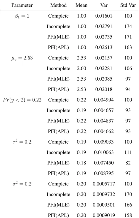
Table2.1presents Monte Carlo mean, variance and standardized variances (which is the ratio of variance and variance of complete sample estimator and times 100) of the point estimators. The incomplete sample estimators are biased for the mean type of the parameters, as expected. From the response model, individuals with largebi values are likely to respond; whereas
indi-viduals with smallbi values are likely to not respond. Thus the observed mean will tend to be
larger than the true mean (in the simulation study, we know the true mean is 2.53) and the ob-served proportion ofy <2will tend to be smaller than the true probability (the true probability is 0.22). On the other hand, the proposed PFI estimators are essentially unbiased in estimating the mean type of parameters. Imputation can largely reduce non-response bias. For estimating variance componentτ2, the imputed ML estimator is biased downward; however the imputed
APL estimator can correct the bias and thus is essentially unbiased for estimating the variance component. The imputation method works well for estimating the variance parameters after incorporating the adjusted profile likelihood idea. PFI (either MLE or APL) is efficient, which can be seen from the Std Var column in Table (2.1) , forµy,P r(y < 2), andτ2, the variance
Parameter Method Mean Var Std Var β1 = 1 Complete 1.00 0.01601 100 Incomplete 1.00 0.02791 174 PFI(MLE) 1.00 0.02735 171 PFI(APL) 1.00 0.02613 163 µy = 2.53 Complete 2.53 0.02157 100 Incomplete 2.60 0.02281 106 PFI(MLE) 2.53 0.02085 97 PFI(APL) 2.53 0.02018 94 P r(y <2) = 0.22 Complete 0.22 0.004994 100 Incomplete 0.19 0.004657 93 PFI(MLE) 0.22 0.004837 97 PFI(APL) 0.22 0.004662 93 τ2 = 0.2 Complete 0.19 0.009033 100 Incomplete 0.19 0.010063 111 PFI(MLE) 0.18 0.007450 82 PFI(APL) 0.19 0.008795 97 σ2 = 0.2 Complete 0.20 0.0005717 100 Incomplete 0.20 0.0009732 170 PFI(MLE) 0.20 0.0009501 166 PFI(APL) 0.20 0.0009019 158
Table 2.1 Mean, variance and standardized variance of the point estimators, based on 2,000 Monte Carlo samples.
Table 2.2 presents the Monte Carlo relative bias and the t-statistics of the variance esti-mators for APL estimator. Variance estiesti-mators of the PFI estiesti-mators are computed using the Louis formula and the linearization method discussed in Appendix. Relative biases of the
vari-ance estimators were computed by dividing the Monte Carlo bias of the varivari-ance estimator by the Monte Carlo variance of the point estimator. The t-statistics are constructed to test the significance of the bias of the variance estimators. A justification of the t-statistics is given in Appendix D of Kim (2004). The variance estimators for PFI are nearly unbiased for the parameters considered.
Parameter Method R.B. (%) t-statistics
β1 PFI(reml) 3.12 1.03 µy PFI(reml) 2.40 0.87
P r(y <2) PFI(reml) 1.31 0.43
Table 2.2 Monte Carlo relative biases and t-statistics of the variance estimator for the impu-tation, based on 2,000 Monte Carlo samples.
2.5
Generalized linear mixed model
Parametric fractional imputation can be extended to generalized linear mixed models. Here we consider the data set on salamander mating, which could be modeled as generalized linear mixed model.
2.5.1 Data description
The salamander data came from the experiment conducted by S. Arnold and P.Verrell (1989), aimed to study the extent to which mountain dusky salamanders from different popu-lations would interbreed. The data given here refer to two popupopu-lations called Rough Butt (R) and Whiteside (W). Forty animals were used in each of three experiments, one conducted in the summer of 1986 and two in the Fall of the same year. The forty salamanders available in each of the three experiments were comprised of 10 Rough Butt males, 10 Rough Butt females, 10 Whiteside males and 10 Whiteside females. Although there were 400 possible crosses between the females and males in each experiment, only 120 of these were permitted
by the design. So totally they observed 360 potential matings. The design of the experiment permits a comparison of the mating probabilities for the four possible crosses: RR, RW, WR and WW.
2.5.2 Generalized linear mixed model
For the total 360 observations in the data set, we consider models for the observed data conditionally on the actual animals used in the experiment. Denoteyij to be a random variable
representing the binary response indicator of a successful mating between theith female and the jth male for i, j = 1,2, . . . ,60 where only 360 of the (i, j) pairs are relevant (each i
corresponds to six j’s). Let ufi denote the random effect that theith female salamander has cross matings in which she is involved, and defineum
j similarly for thejth male. Letxij denote
a 4 dimensional vector of covariates indicating the type of cross for the mating pair between femaleiand malej . We assume that theyij0 s are all conditionally independent, and assume a Binomial regression model for the salamander data set, i.e.,
yij|u f i, u m j ∼Bernoulli(πij), (2.14) and ηij =g(πij) =logit(πij) = xTijβ+u f i +u m j , (2.15)
where g(·) is the link function, and we use the canonical link which is the logit link, β = (βRR, βRW, βW R, βW W)T is an unknown4dimensional regression parameter vector. The
pa-rameter vectorβas fixed effects andufi ’s andum
j ’s as random effects. Assumeu f
i ∼N(0, σ2f)
andum
j ∼N(0, σm2), so the resulting model has 6 unknown parametersβRR, βRW, βW R, βW W,
σ2
f andσm2.
Let y denote the full data vector, and let uf, um be two 60-variate random variables with parametric densities g1(uf|σ2f) and g2(um|σm2) respectively. The joint distribution of
(y,uf,um)is Y60 i=1 i6 Y j=i1 πyij ij (1−πij)1−yij g1(uf|σf2)g2(um|σm2), (2.16)
whereπij =g−1(xTijβ+u f i +umj ) = exp(xT ijβ+u f i+u m j ) 1+exp(xT ijβ+u f i+umj ) .
The likelihood function forγ = (β, σ2
f, σ2m)is L(γ|y) = ˆ ˆ Y60 i=1 i6 Y j=i1 πyij ij (1−πij)yij g1(uf|σf2)g2(um|σ2m)du fdum. (2.17)
The likelihood functionL(γ|y)involves intractable integrals whose dimension depends on the structure of the random effects(uf,um)which is a 120-dimensional vector, so likelihood
inference requires numerical evaluation of a high-dimensional integral.
2.5.3 Fractional Imputation
The complete log-likelihood function ofγ= (β, σ2
f, σm2)is given by lcom(γ) = 60 X i=1 i6 X j=i1 {yijlogπij + (1−yij) log(1−πij)} + logg1(uf|σf2) + logg2(um|σm2).
We treat the random effects(uf,um)as missing data. The maximum likelihood estimator ˆ
γ can be obtained by maximizing
Q(γ) =E{lcom(γ;y,uf,um)|y}.
In the above expectation, the reference distribution is the conditional distributionuf,um|y,
uf,um|y∝ 60 Y i=1 i6 Y j=i1 πyij ij (1−πij)yij g1(uf|σf2)g2(um|σ2m).
We consider a 120-dimensional multivariate Student t importance density (suggested by Booth and Hobert, 1998) with 3 degrees of freedom, whose mean and variance match the mode and curvature of the target distribution f(u|y;γ), u = (uf,um). Write f(u|y;γ) =
aexp{l(u)},whereais the normalizing constant. Letl(i)(u)be theith derivative ofl(u), andu˜
of the mean and variance areu˜ and−l(2)(u˜). See Booth and Hobert (1998) for the formula.
Denoteu∗(1), . . . ,u∗(M)as a random sample fromh(u|ν, µ,Σ), which is a multivariate Student
t distribution withν= 3,µ= ˜uandΣ=−l(2)(˜u), the fractional weights are given by w∗(k)(γ) = f(y,u
∗(k)|γ)/h(u∗(k)|ν, µ,Σ) PM
l=1f(y,u∗(l)|γ)/h(u∗(l)|ν, µ,Σ) .
The Monte Carlo approximate of the observed likelihood function is given by
Q∗(γ|γ(t)) = M
X
k=1
w∗(k)(γ(t)) logf(y,u∗(k)|γ),
which is maximized in each M-step in the EM algorithm to update the parameter estimatesγ(t)
toγ(t+1). Method βRR βRW βW R βW W σf2 σ2m Pseudo lik 0.78 0.24 -1.48 0.77 0.65 0.58 Imputation 0.97 0.33 -1.81 0.95 1.13 0.89 MLE 1.01 0.31 -1.90 0.99 1.17 1.04 MCEM 1.02 0.32 -1.94 0.99 1.39 1.23 Gibbs 1.03 0.34 -1.98 1.07 1.49 1.37 Table 2.3 Salamander Data set (observations=360)
Table 4.2 shows the results from PFI and various estimation methods, including Pseudo likelihood method (Arnold and Verrel), MLE from a modified EM algorithm with Laplace ap-proximation (Steele, 1996), Gibbs sampling method (Karim and Zeger, 1992) and the Monte Carlo EM method (Vaida and Meng, 2005). Ver Hoef et. al (2010) suggested the Pseudo like-lihood approach to create a linear mixed pseudo-model where the resulting estimator is called pseudo likelihood estimator. Pseudo-likelihood estimates can be implemented in SAS GLIM-MIX procedure. As we can see, the estimates of parameters in the pseudo-likelihood approach are quite different from other approaches which is caused by the lack of efficiency of pseudo-likelihood approximation to the original pseudo-likelihood when a large dimension of random effects
are involved. Steele (1996) suggests replacing the conditional expectation in the E-step with a second order approximation and this modified EM algorithm produced accurate estimates of the fixed effects in generalized linear mixed models. Our imputation method gives estimates close to MLE. The Gibbs sampling approach and the Monte Carlo EM method tend to produce larger estimates than MLE. However, as we discussed previously, both methods involve heavy computation which is not desirable in practice. The PFI samples are created only once in the beginning of EM algorithm and thus largely reduce the burden of computation. This exam-ple shows that statistically efficient estimation is possible without requiring a computationally extensive method.
2.6
Discussion Remark
Parametric fraction imputation is proposed as a general tool for estimation with missing clustered data. If the parametric fractional imputation is used to construct the score function, the solution to the imputed score equation is very close to the maximum likelihood estimator for the parameters in the model. The imputation method is applicable to the restricted maxi-mum likelihood method or the adjusted profile likelihood method. The variance estimator can be obtained from a Taylor linearization. PFI can also be easily extended to generalized linear mixed model, which allows statistically efficient estimation without requiring a computation-ally extensive method and can be more feasible in practice.
2.7
Appendix section - Variance estimation
Since β and θ are information orthogonal, we can use Louis’s formula to construct the confidence intervals forβ.
Iobs(β) =− n X i=1 ES˙(β;yi)|yi,obs − n X i=1 VS(β;yi)|yi,obs . (2.18)
which can be approximated by − n X i=1 M X k=1 w∗i(k)S˙( ˆβ;y∗i(k))− n X i=1 M X k=1 wi∗(k) S( ˆβ;yi∗(k))−Si¯( ˆβ) ⊗2. (2.19)
whereS(β;y) =∂logf(y;β)/∂β,S˙(β;y) = ∂S(β;y)/∂βandS¯i(β) =
PM k=1w ∗(k) i S(β;y ∗(k) i ).
For variance estimation of ηˆ, based on Taylor linearization obtained from U¯∗(η) = 0 in (2.9), we can writeU¯(η|γˆ)≈U¯(η0|γ0) +K0S¯(γ0), whereKis defined as
K =−[E{∂S¯(γ0)/∂γ}]−1E{Smis(γ0)U(η0)}. If we write ¯ U(η|γ) +K0S¯(γ) =n−1 n X i=1 {u¯i(η|γ) +K0¯si(γ)}=n−1 n X i=1 ˜ ui.
the plug-in estimator of Var(Pn
i=1u˜i)is
Pn
i=1(ˆui−u¯ˆ)(ˆui−u¯ˆ)0, whereuˆi = ¯ui(ˆη; ˆγ)+ ˆK0¯si(ˆγ).
The terms u¯i(ˆη; ˆγ) and ¯si(ˆγ) can be computed from fractional imputation with fractional
Bibliography
[1] BARNDORFF-NIELSEN, O.E. (1986), “Inference on full and partial parameters based on
the standardized signed log likelihood ratio,” Biometrika,73, 307–22.
[2] BOOTH, J.G.ANDHOBERT, J.P. (1999). “Maximizing generalized linear models with an automated Monte Carlo EM algorithm,” Journal of the Royal Statistical Society: Series B,61, 625–85.
[3] CHAN, J.S.K.,ANDKUK, A.Y.C. (1997). “Maximum Likelihood Estimation for Probit-linear Mixed Models with Correlated Random Effects,” Biometrics,53, 86–7.
[4] COX, D.R. AND REID, N. (1987). “Parameter orthogonality and approximate
condi-tional inference (with discussion),” Journal of the Royal Statistical Society: Series B,
49, 1–39.
[5] DIGGLE, P.J.ANDKENWARD, M.G. (1994). “Informative drop-out in longitudinal anal-ysis,” Applied Statistics,43, 49–93.
[6] FOLLMANN, D.A.ANDWU, M.C. (1995). “An Approximate Generalized Linear Model
with Random Effects for Informative Missing Data,” Biometrics,51, 151–168.
[7] GREENLEES, J.S.ANDZIESCHANG, K.D. (1982). “Imputation of missing values when
the probability of response depends on the variable being imputed,” Journal of the Amer-ican Statistical Association,77, 251–61.
[8] IBRAHIM, J.G., LIPSITZ, S.R.AND CHEN, M. (1999). “Missing covariates in
general-ized linear models when the missing data mechanism is nonignorable,” Journal of the
Royal Statistical Society: Series B,61, 173–90.
[9] KARIM, M.R. AND ZEGER, S.L. (1992). “Generalized linear models with random
ef-fects: salamander mating revisited,” Biometrics,48:631–644.
[10] KIM, J.K. (2004). “Finite sample properties of multiple imputation estimators,” The Annals of Statistics,32: 766–783.
[11] KIM, J.K. (2011). “Parametric fractional imputation for missing data analysis,” Biometrika,98, 119–132.
[12] LITTLE, R.J.A. (1995). “Modeling the drop-out mechanism in repeated-measures
stud-ies,” Journal of the American Statistical Association,90, 1112–1121.
[13] MCCULLOCH, C.E. (1997). “Maximum likelihood algorithms for generalized linear
mixed Models,” Journal of the American Statistical Association,42, (437) 162–70. [14] MCCULLAGH, P. AND NELDER, J.A. (1989). “Generalized linear models”. Ghapman
and Hall, pages 441–450.
[15] MOLENBERGHS, G.ANDKENWARD, M.G. (2007). “Missing Data in Clinical Studies,” Wiley.
[16] PATTERSON, H. D.ANDTHOMPSON, R. (1971). “Recovery of inter-Block Information
when Block sizes are unequal,” Biometrika,58, 545–554.
[17] STEELE, B.M. (1996). “A modified EM algorithm for estimation in generalized mixed
models,” Biometrics,52:1295–1310.
[18] TEN HAVE, T., KUNSELMAN, A., PULKSTENIS, E. AND LANDIS. J. (1998). “Mixed
Effects Logistic Regression Models for Longitudinal Binary Response Data with Infor-mative Drop-Out,” Biometrics,54, 367–383.
[19] TROXEL, A.B., HARRINGTON, D.P.ANDLIPSITZ, S.R. (1998). “Analysis of
longitudi-nal measurements with nonignorable non-monotone missing values,” Applied Statistics,
47, 425–438.
[20] VAIDA, F. AND MENG, X.L. (2005). “Two slice-EM algorithms for fitting generalized linear mixed models with binary response,” Statistical Modelling,5, 229–242.
[21] VERHOEF, J.M., LONDON, J.M.ANDBOVENG, P.L. (2010). “Fast computing of some generalized linear mixed pseudo-models with temporal autocorrelation,” Comput Stat,
25, 39–55.
[22] WEI, G.C.G. AND TANNER, M.A. (1990). “A Monte Carlo implementation of the EM
algorithm and the poor man data augmentation algorithm,” Journal of the American Statistical Association,85, 699–04.
[23] WU, M.C. ANDCARROLL, R.J. (1988). “Estimation and comparision of changes in the presence of informative right censoring by modeling the censoring process,” Biometrics,
44, 175–188.
[24] ZEGER, S.L. AND KARIM, M.R. (1991). “Generalized linear models with random
ef-fects: A Gibbs sampling approach,” Journal of the American Statistical Association,86: 79–86.
CHAPTER 3. IMPUTATION METHODS FOR QUANTILE
ESTIMATION UNDER MISSING AT RANDOM
A paper is published inStatistics and Its Interface1
Shu Yang2, Jae Kwang Kim3, and Dong Wan Shin4
abstract
Imputation is frequently used to handle missing data for which multiple imputation is a popular technique. We propose a fractional hot deck imputation which produces a valid vari-ance estimator for quantiles. In the proposed method, the imputed values are chosen from the set of respondents and are assigned with proper fractional weights that use a density function for the working model. In addition, we consider a nonparametric fractional imputation method based on nonparametric kernel regression, avoiding a parametric distribution assumption and thus giving more robustness. The resulting estimator can be called nonparametric fractionally imputation estimator. Valid variance estimation is also discussed. A limited simulation study compares the proposed methods favorably with other existing methods.
3.1
Introduction
Quantile estimation is frequently used in many disciplines. In industry, a device man-ufacturer may wish to know what are the 10% and 90% quantiles for some features of the
1Reprinted with permission of Statistics and Its Interface,2013,6, 369–377. 2Primary researcher and author.
3Author for correspondence. 4Author for correspondence.
production processes to tailor the process to produce 80%of the devices. In finance, for risk management, a bank may need to estimate a lower bound on the changes in the values of its portfolio which will hold with high probability.
We consider imputation methods for quantile estimation, where the missing mechanism is assumed to be missing at random in the sense of Rubin (1987). Under existence of missing data, imputation is often used for missing data analysis to facilitate the parameter estimation, which is a process of replacing missing values with pseudo values so that analysis from differ-ent users will be consistdiffer-ent.
There are various ways to impute missing values which lead to different imputation meth-ods. Multiple imputation (MI in the sequel), proposed by Rubin (1987), uses a Bayesian method to generate imputed values to represent the uncertainty about the right value to impute. Parametric fractional imputation (PFI in the sequel), proposed by Kim (2011), is a frequentist version of the MI, where fractional weights are assigned to the imputed values to properly represent the point mass of the imputed values.
Imputation has been widely used for handling missing data because a single imputed data can be used to estimate several parameters. However, many papers on imputation focused only on estimating the population mean. Estimating the population quantiles with imputed data is also an important practical problem but has rarely addressed in the literature. We discuss the MI and PFI in terms of quantile estimation. Moreover, we propose a new imputation method which can be called fractional hot deck imputation (FHDI in the sequel). Instead of generating imputed values, FHDI chooses the imputed values from the set of respondents and assigns fractional weights to imputed values so that the conditional expectation of the estimating function is approximated by the imputed estimating function.
The proposed FHDI method has a nonparametric feature which can easily modified to a fully nonparametric version called nonparametric fractional imputation (NPFI in the sequel). In NPFI, the whole estimation procedure is fully nonparametric. On the other hand, MI and PFI rely on the model assumptions. Therefore, the proposed methods, FHDI and NPFI, are
more robust than the existing methods, MI and PFI, producing less-biased estimators in the cases of failure of the assumed model.
More important advantage of the fractional imputation methods over the MI method is that the former allow valid variance estimators for quantile estimates while for the latter variance estimator using Rubin’s formula is not valid. Valid variance estimation for fractional imputa-tion is possible because, unlike MI, the effect of estimated nuisance parameter in imputaimputa-tion is correctly reflected in the replication variance estimation. It is well known that direct applica-tion of delete-1 observaapplica-tion jackknife variance estimaapplica-tion is not valid for medians or quantiles. On the other hand, FHDI and NPFI allow a valid two-step variance estimator of quantiles by combining the linearization method (or test inversion method) and the delete-1 observation jackknife variance estimation to the empirical distribution function together.
The rest of the paper is organized as follows. In section 2, we introduce multiple imputation and parametric fractional imputation in quantile estimation with ignorable missing data. In section 3, we develop FHDI and NPFI for quantile estimation. Delete-1 observation jackknife variance estimation is discussed in Section 4. Section 5 presents a limited simulation study and a real data set analysis. Some concluding remarks follow in Section 6.
3.2
Existing Methods
When the study variableyis fully observed in the sample, an empirical distribution function can be computed from the sample by
ˆ F(y) = n−1 n X i=1 I(yi < y),
and the sample quantile is then computed by the inverse of empirical distribution
ˆ
ξp = ˆF−1(p) = inf{y: ˆF(y)≥p},
which can also be viewed as a solution to the estimating equation
U(ξp) = n X i=1 U(ξp, yi) = n−1 n X i=1 {I(yi < ξp)−p}= 0.
The above estimation procedure is robust because it does not require any distribution assump-tion.
For variance estimation, we consider two types of variance estimators. The first type is the linearization method estimator which is based on the Bahadur representation (Bahadur, 1966).
ˆ V( ˆξp)∼= 1 [ ˆf( ˆξp)]2 ˆ V( ˆF( ˆξp,F I)), (3.1)
where f is the marginal density function of Y. The second type is the Woodruff variance estimator (Woodruff 1952) which is based on the so-called test-inversion method. To compute the Woodruff variance estimator, we first construct a normal-based 95% asymptotic confidence interval forpbypˆ±2
q
ˆ
V(ˆp)≡ (ˆpL,pˆU), wherepˆ≡Fˆ( ˆξp). SinceFˆ is monotone, a
normal-based 95% asymptotic confidence interval forξp can be obtained by ( ˆF−1(ˆpL),Fˆ−1(ˆpU)) ≡ ( ˆξp,L,ξˆp,U). Thus the Woodruff variance estimator is given by
ˆ V( ˆξp) = ˆ ξp,U−ξˆp,L 4 2 . (3.2)
We now consider missing cases. Several imputation methods will be adopted to estimate the quantiles. We assume that the study variable y is subject to missing and an auxiliary variablexis observed throughout the sample. Properly incorporatingxinto the estimation of the quantiles ofycan lead to bias correction as well as variance reduction. For simplicity, we assume that the firstrelements have bothxandyobserved and the remainingn−relements have onlyxobserved.
3.2.1 Multiple Imputation (MI)
Multiple imputation (MI) is a popular technique of imputation proposed by Rubin (1987). In the MI, instead of generating one single value, a set of plausible values are generated to represent the uncertainty about the right value to impute. The complete sample estimator is then applied to each of the multiply imputed data sets. Finally the results are combined from these analysis for inference.
In MI, Bayesian method is used to generate imputed values. Multiple imputation procedure for bivariate normal(x, y)is described in Schenker and Welsh (1988). At each repetition of the imputation(k = 1, ..., m), we can calculate the imputed version of the quantile estimator
ˆ
ζγ,I(k)and its variance estimatorVˆI(k). The final quantile estimator is computed by
ˆ ζγ,M I =m−1 m X k=1 ˆ ζγ,I(k).
Rubin proposed using the following estimator for the variance ofζˆγ,M I: ˆ VM I =Wm,n+ 1 +m−1 Bm,n, (3.3) where Wm,n =m−1 m X k=1 ˆ VI(k), (3.4) and Bm,n = (m−1) −1 m X k=1 ˆ ζγ,I(k)−ζˆγ,M I 2 . (3.5)
In (3.4),VˆI(k)is the variance estimator (3.1) or (3.2) applied to thekthimputed data set.
Validity of the MI variance estimator requires that the congeniality condition of Meng (1994) holds. Roughly speaking, the congeniality condition means that
V(ˆθM I) =V(ˆθn) +V(ˆθM I−θˆn).
Kim (2011) argues that the congeniality condition does not hold when the parameter of inter-est is θ = P r(Y < c) andθˆn = n−1Pni=1I(yi < c) is used to estimate θ under complete
response. Because the quantile estimator is also obtained from the sample distribution func-tion, the congeniality condition does not hold for quantiles, which is confirmed numerically in the simulation study in Section 5.
3.2.2 Parametric Fractional Imputation (PFI)
Parametric fractional imputation (PFI) was proposed by Kim (2011) for general purpose estimation. In Kim (2011), the PFI method was developed for estimating population mean
and proportion under ignorable non-response. The PFI method can be developed for quantile estimation as well. One advantage of the PFI method is that, if the imputed data is applied to the score function or the estimating function, the resulting estimator is very close to the maximum likelihood estimator. In the PFI method, m imputed values are generated for yi,
i=r+ 1, . . . , nandmfractional weights are assigned to the imputed values so that the mean score function or the mean estimating function can be approximated by a weighted sum of the imputed score functions or estimating functions. Letyij∗ be thejth imputed value of missing
yi andw∗ij be the fractional weight assigned toy
∗
ij. The fractional weights are constructed to
satisfy
m
X
j=1
w∗ij = 1, (3.6) for eachi= 1,2, . . . , nand
w∗ij ∝ f(y ∗ ij|xi; ˆθ) h(y∗ ij) , (3.7)
wheref(y | x;θ)is the conditional density of y givenx, h(y)is the density function of the distribution from whichyij∗ are generated,θˆis the MLE ofθwhich is obtained by solving
r
X
i=1
S(θ;xi, yi) = 0,
andS(θ, xi, yi) = ∂logf(yi|xi, θ)/∂θis the score function for thei−th observation,f(yi|xi, θ).
Once the fractional weights are constructed, the PFI estimator ofξp is given by ˆ ξp,P F I∗ = ˆFP F I∗−1(p) = inf{y: ˆFP F I∗ (y)≥p}, (3.8) where ˆ FP F I∗ (y) =n−1 n X i=1 {δiI(yi < y) + (1−δi) m X j=1 wij∗I(y∗ij < y)}. (3.9) andδi is the response indicator such thatδi = 1for observedyi andδi = 0for missingyi.
Variance estimation can be obtained by the linearization method as described in Appendix A.1.
3.3
Proposed methods
In MI and PFI, the imputed values are generated from a parametric distribution. Instead of generating imputed values, in the FHDI, the imputed values are taken from the set of respon-dents. The record providing the value is called the donor and the record with the missing value is called the recipient. Hot deck imputation is initially proposed by Brick and Kalton (1996) to reduce imputation variance by random selection of one imputed value among donors. Kalton and Kish (1984) and Fay (1996) used more than one donor for a recipient to reduce the impu-tation variance.
3.3.1 Fractional hot deck imputation (FHDI)
In FHDI, for each missingyi, a set ofmimputed values{y∗i1, . . . , yim∗ }are obtained from
the set of respondents{y1, ..., yr}, i =r+ 1, ..., n. Letw∗ij be the fractional weights assigned
toy∗ij,j = 1,2, . . . , m. In FHDI, we usem =r, that is, thej-th imputed value of missingyiis
y∗ij = yj, an observed value, j = 1, ..., r. In this case, the fractional weightsw∗i1, . . . , w ∗ ir are computed to satisfyPr j=1w ∗ ij = 1and r X j=1 w∗ijI(yj < y)∼=P r(yi < y|xi).
Since we can treat {y1,· · · , yr} as a set of realizations fromf(y | δ = 1), the desired
fractional weight assigned toy∗ij =yj forδi = 0is given by
w∗ij ∝ f(yj|xi; ˆθ) f(yj|δj = 1) , (3.10) andPm j=1w ∗ ij = 1, fori=r+ 1, . . . , n. Since f(y|δ= 1) = ˆ f(y|x, δ= 1)f(x|δ= 1)dx = ˆ f(y|x)f(x|δ= 1)dx,
where the second equality follows from MAR, a consistent estimator off(yj|δj = 1)is given by ˆ f(yj|δj = 1) = Pn k=1δkf(yj|xk,θˆ) Pn k=1δk ,
which uses the empirical distribution forf(x|δ= 1). That is, it uses
ˆ f(x|δ = 1) = P δi=1I(x=xi) Pn i=1δi . (3.11) Thus, the fractional weight in (3.10) is computed by
wij∗ = f(yj|xi; ˆθ)/{ Pn k=1δkf(yj|xk,θˆ)} Pr l=1[f(yl|xi; ˆθ)/{ Pn k=1δkf(yl|xk,θˆ)}] .
Once the weight set {wij∗}is created, the FHDI estimatorξˆp,F HDI ofξp is computed from
(3.8) - (3.9) with these{w∗ij}replacing that in (3.8) - (3.9). Variance estimation forξˆp,F HDI
will be discussed in Section 4.
3.3.2 Nonparametric fractional imputation (NPFI)
Fractional imputation can be implemented nonparametrically. Cheng (1994) used kernel regression estimators to estimate mean functionals through empirical estimation of the miss-ing pattern. Chen (2001) and Kim and Yu (2011) used a semi-parametric logistic regression model of mean functionals with non-ignorable missing data. We adopt the kernel regression idea to obtain fractional weights in FHDI, and the resulting imputation method will be called nonparametric fractional imputation, NPFI.
Let K(·) be a symmetric density function on the real line and h = hn be a smoothing
bandwidth such thathn→0andnhn→ ∞asn→ ∞. A nonparametric regression estimator
ofm(x) =E(y|x)can be obtained by findingmˆ(x)that minimizes
n
X
i=1
Kh(xi, x)δi{yi−m(x)}2,
where Kh(u, x) = h−1K{(u−x)/h}. The minimizer is the well-known Nadaraya-Watson
(1964) kernel regression estimator (NW estimator)
ˆ m(x) = n X j=1 wj1(x)yj,
where wi1(x) = Kh(x, xi)δi Pn j=1Kh(x, xj)δj , (3.12) which represents the point mass assigned toyi whenm(x)is approximated byPim=1wi1(x)yi.
Considermˆ(xi)to be a prediction for missing uniti, then
ˆ µy = n−1 n X i=1 {δiyi+ (1−δi) ˆm(xi)} = n−1 n X i=1 {δiyi+ (1−δi) n X j=1 wj1(xi)yj}.
The weight w∗ij = wj1(xi) is essentially the fractional weight assigned to jth imputed value
for missing uniti. Consider implementing fractional hot deck imputation in a nonparametric fashion. Using (3.10) wheref(yj|xi)is nonparametrically estimated by a kernel-based method,
the final fractional weights can be given by
w∗ij = PnKh(xi, xj)/C(xj) k=1Kh(xi, xk)δk/C(xk) , where C(xj) = n X i=1 δiKh(xi, xj).
Given the weight set {wij∗}, the NPFI estimator ξˆp,N P F I is computed from (3.8) - (3.9) with
these{w∗ij}replacing that in (3.8) - (3.9). Variance estimation forξˆp,N P F I will be discussed in
Section 4.
3.4
Variance estimation
One advantage of FHDI and NPFI is that all imputed values are realized values, which en-ables us to use the replication method for variance estimation. Delete-1 observation jackknife variance estimator is considered. It has been shown that delete-1 observation jackknife vari-ance estimator is valid with smooth differentiable statistics, such as totals, means, proportions and etc; but not with medians or quantiles.
In order to get a valid variance estimator in FHDI and NPI, we consider a two-step pro-cedure using the linearization method or the test inversion method in the first step and the delete-1 observation jackknife variance estimation with the empirical distribution function in the second step. This two-step approach makes the delete-1 observation jackknife variance estimator valid for median or quantile estimators.
Denote HD as either FHDI or NPFI. Based on the linearizaiton method of (3.1) applied to
ˆ ξp,HD= ˆFHD−1(p), we get V( ˆξp,HD)∼= 1 [ ˆf( ˆξp,HD)]2 V{FˆHD( ˆξp,HD)},
or the test inversion method of (3.2), we get
V( ˆξp,HD) = ˆ ξp,U −ξˆp,L 4 !2 , where(ˆpL,pˆU) = ˆFHD( ˆξp,HD)±2 q V( ˆFHD( ˆξp,HD)), and( ˆξp,L,ξˆp,U) = ( ˆF−1(ˆpL),Fˆ−1(ˆpU)).
In either method, we need a consistent estimate ofV( ˆFHD( ˆξp,HD)).
Notice thatFˆHD(y) = n−1 Pn i=1{δiI(yi < y) + (1−δi) Pm j=1w ∗ ijI(y ∗ ij < y)}is a
propor-tion. CreateZi =I(yi <ξˆp,HD)andZij∗ =I(yij∗ <ξˆp,HD). Then
ˆ FHD( ˆξp,HD) = ¯ZHD =n−1 n X i=1 {δiZi+ (1−δi) m X j=1 wij∗Zij∗}.
So, Jackknife method can be applied to obtain a consistent estimator for the variance of the average FˆHD( ˆξp,HD) = ¯ZHD. Specifically, V{FˆHD( ˆξp,HD)} = V( ¯ZHD)is estimated by the
following delete-1 observation jackknife variance estimator
ˆ Vrep{FˆHD( ˆξp,HD)}= n−1 n n X k=1 ( ¯ZHD(k) −Z¯HD)2, where ¯ ZHD(k) =n−1 n X i=1 {δiw (k) i Zi+ (1−δi) m X j=1 wj(k)w∗ij(k)Zij∗},
with wi(k)= (n−1)−1 if i6=k 0 if i=k .
For FHDI,w∗ij(k)are the replicate fractional hot deck weights computed by wij∗(k)= w (k) j f(yj|xi; ˆθ(k))/{ Pn l=1w (k) l δlf(yj|xl; ˆθ(k))} Pm s=1[w (k) s f(ys|xi; ˆθ(k))/{Pnl=1wl(k)δlf(ys|xl; ˆθ(k))}] . Thek-th replicate ofθˆ, denoted byθˆ(k), satisfies
r
X
i=1
wi(k)S(ˆθ(k);xi, yi) = 0.
For NPFI,w∗ij(k)are the replicate nonparametric fractional weights computed by
w∗ij(k)= w (k) j Kh(xi, xj)/C(k)(xj) Pn l=1{w (k) l Kh(xi, xl)/C(k)(xl)} , whereC(k)(xj) = Pn i=1δiw (k) i Kh(xi, xj).
Once we obtain the delete-1 observation jackknife variance estimator Vˆrep{FˆHD( ˆξp,HD)}
ofV {FˆHD( ˆξp,HD)}, we can get a consistent variance estimator ofξˆp,HD. If the linearizaiton
method is used, we get the variance estimator ofξˆp,HDas ˆ V( ˆξp,HD)∼= 1 [ ˆf( ˆξp,HD)]2 ˆ Vrep{FˆHD( ˆξp,HD)}. (3.13)
If the test inversion method is used, we get the variance estimator ofξˆp,HD as ˆ V( ˆξp,HD) = ˆ ξp,U −ξˆp,L 4 !2 , (3.14) where( ˆξp,L,ξˆp,U) = ( ˆF−1(ˆpL),Fˆ−1(ˆpU)),(ˆpL,pˆU) = ˆFHD( ˆξp,HD)±2 q ˆ Vrep{FˆHD( ˆξp,HD)}.
3.5
Simulation Study
We performed a limited simulation study and a real data analysis. In Section 5.1, we compared the performance of the proposed method with some other imputation methods in a correctly specified model and a misspecified model. In Section 5.2, we applied FHDI to a real data analysis from the Korea Labor and Income Panel Survey (KLIPS).
3.5.1 Simulation
Two sets of models were considered to generate the observations. In Model A, we used
yi = 1 +xi +ei, where xi ∼ N(0,1),ei ∼ N(0,1), xi andei are independent. In Model B,
we usedyi = 1 +xi +ei, wherexi ∼ N(0,1), ei ∼ Exp(1)−1, xi andei are independent.
Random samples of sizen= 200were separately generated from the two models. In addition to(xi, yi), we also generatedδi, the response indicator variable, from Bernoulli distributions
with response rate0.6. Variablexiis always observed but variableyiis observed if and only if
δi = 1. We usedB = 2,000Monte Carlo samples in the simulation. In each of the samples,
we computed the following five estimators:
1. Full sample (Full) estimator that is computed using the complete observations.
2. Multiple imputation (MI) estimator with imputation size m, where the imputed values are generated from the normal-theory regression model, as considered in Schenker and Welsh (1988).
3. Parametric fractional imputation (PFI) estimator with imputation sizem.
4. Fractional hot deck imputation (FHDI) estimator using the full set of respondents as imputation values (m=nr) wherenr is the size of respondents.
5. Nonparametric fractional imputation (NPFI) estimator.
In MI and PFI, we set the imputation sizem=nr, the same as that in FHDI, for fair
compari-son. In both Model A and B, we used a working model which is the normal density with mean
β0+β1xand varianceσ2as the imputation model. Thus, the working model is the true model
in model A but not true in model B. In NPFI, the nonparametric kernel regression estimator was computed using a Gaussian kernel function with bandwidth h = an−2/5, suggested by