Syracuse University Syracuse University
SURFACE
SURFACE
Electrical Engineering and Computer Science -
Dissertations College of Engineering and Computer Science
5-2013
Rank Based Anomaly Detection Algorithms
Rank Based Anomaly Detection Algorithms
Huaming HuangSyracuse University
Follow this and additional works at: https://surface.syr.edu/eecs_etd
Part of the Computer Engineering Commons
Recommended Citation Recommended Citation
Huang, Huaming, "Rank Based Anomaly Detection Algorithms" (2013). Electrical Engineering and Computer Science - Dissertations. 331.
https://surface.syr.edu/eecs_etd/331
This Dissertation is brought to you for free and open access by the College of Engineering and Computer Science at SURFACE. It has been accepted for inclusion in Electrical Engineering and Computer Science - Dissertations by an authorized administrator of SURFACE. For more information, please contact [email protected].
Anomaly or outlier detection problems are of considerable importance, arising frequently in diverse real-world applications such as finance and cyber-security. Several algorithms have been formulated for such problems, usually based on formulating a problem-dependent heuristic or distance metric. This dissertation proposes anomaly detection algorithms that exploit the notion of “rank," expressing relative outlierness of different points in the rele-vant space, and exploiting asymmetry in nearest neighbor relations between points: a data point is “more anomalous" if it is not the nearest neighbor of its nearest neighbors. Al-though rank is computed using distance, it is a more robust and higher level abstraction that is particularly helpful in problems characterized by significant variations of data point density, when distance alone is inadequate.
We begin by proposing a rank-based outlier detection algorithm, and then discuss how this may be extended by also considering clustering-based approaches. We show that the use of rank significantly improves anomaly detection performance in a broad range of prob-lems.
We then consider the problem of identifying the most anomalous among a set of time series, e.g., the stock price of a company that exhibits significantly different behavior than its peer group of other companies. In such problems, different characteristics of time series are captured by different metrics, and we show that the best performance is obtained by combining several such metrics, along with the use of rank-based algorithms for anomaly detection.
In practical scenarios, it is of interest to identify when a time series begins to diverge from the behavior of its peer group. We address this problem as well, using an online version of the anomaly detection algorithm developed earlier.
within a single time series. This is accomplished by refining the multiple-distance combina-tion approach, which succeeds when other algorithms (based on a single distance measure) fail.
The algorithms developed in this dissertation can be applied in a large variety of appli-cation areas, and can assist in solving many practical problems.
ALGORITHMS
ByHuaming Huang
B.S. Xiamen University, 2000 M.S. Syracuse University, 2009 DISSERTATIONSubmitted in partial fulfillment of the requirements for the degree of
Doctor of Philosophy in Computer and Information Science and Engineering (CISE)
Syracuse University May 2013
Copyright c2013 Huaming Huang All rights reserved
List of Tables xi
List of Figures xiv
1 Introduction 1
1.1 What are outliers? . . . 1
1.2 Types of Outliers Detection Problems . . . 3
1.3 Our Goals . . . 8
1.4 Point Outlier Detection for Static data set . . . 8
1.4.1 Existing Approaches . . . 9
1.4.2 Drawbacks in Density-based Approaches . . . 11
1.4.3 Our Solution . . . 11
1.4.4 Our Contributions . . . 12
1.5 Outlier Detection for Time Series Data Sets . . . 13
1.5.1 Anomalous Time Series Detection . . . 14
1.5.2 Abnormal Subsequences Detection in a Single Series . . . 16
1.6 Online (Real-time) Anomalous Series Detection . . . 17
1.6.1 Related Research . . . 17
1.6.2 Our Solutions . . . 18
2 Point Outliers Detection Based On Ranks 19 2.1 Review of Density-based Approaches . . . 19
2.1.1 LOF (Local Outlier Factor) approach . . . 20
2.1.2 COF (Connectivity-based Outlier Factor) approach . . . 21
2.1.3 INFLO (INFLuential measure of Outlierness by symmetric rela-tionship) approach . . . 24
2.2 Rank-Based Detection Algorithm (RBDA) . . . 25
2.2.1 Description of Rank-based Detection Algorithm (RBDA) Algo-rithm . . . 27
2.2.2 Why does RBDA work? . . . 29
2.3 Experiments: . . . 31
2.3.1 Metrics for Measurement . . . 31
2.3.2 Synthetic Datasets . . . 32
2.3.3 Real Datasets: . . . 36
2.3.4 Real Datasets with Rare Classes . . . 36
2.3.5 Real Datasets with Planted Outliers . . . 38
2.3.6 Conclusions . . . 40
3 Anomaly Detection Algorithms Based on Clustering and Weighted Ranks 41 3.1 Clustering Approach for Anomaly Detection and a New Clustering Algorithm 42 3.2 Notation and Definitions . . . 43
3.3 Neighborhood Clustering (NC-clustering) . . . 44
3.3.1 Density and Rank Based Detection Algorithms . . . 46
3.4 New algorithms based on distance and cluster density . . . 47
3.4.1 Rank with Averaged Distance Algorithm (RADA) . . . 48
3.4.2 Outlier detection using modified-ranks (ODMR) . . . 49
3.4.3 Algorithm Description . . . 51
3.5 Experiments . . . 52
3.5.1 Results . . . 53
3.6 Conclusions . . . 55
4.1 Problem Definition Revisit . . . 58
4.2 Existing Approaches - A Revisit . . . 58
4.3 Outlier Detection Based on Multiple Distance Measures - MUDIM . . . 63
4.3.1 Measure Selection . . . 63
4.3.2 Anomaly Detection Based on Selected Measures . . . 65
4.3.3 Normalization . . . 67
4.3.4 Assignment of Weights to Selected Measure . . . 68
4.3.5 Decision for Anomalous Series . . . 68
4.3.6 Evaluation Methods . . . 69
4.4 Datasets and Results . . . 71
4.4.1 Datasets . . . 71
4.4.2 Experiment Results . . . 81
4.5 Conclusion . . . 81
5 Online Anomalous Time Series Detection 83 5.1 Problem Statement . . . 83
5.2 Literature Review . . . 84
5.3 Online MUDIM Algorithms . . . 85
5.3.1 A Naive Online MUDIM Algorithm (NMUDIM) . . . 85
5.3.2 Faster Online Detection of MUDIM (OMUDIM) . . . 89
5.4 Experiments . . . 90
5.4.1 Results . . . 91
5.4.2 Time Complexity . . . 93
5.5 Concluding Remarks . . . 94
6 Abnormal Subsequence Detection in a Single Series 95 6.1 Problem Statement . . . 95
6.2 Literature Review . . . 96
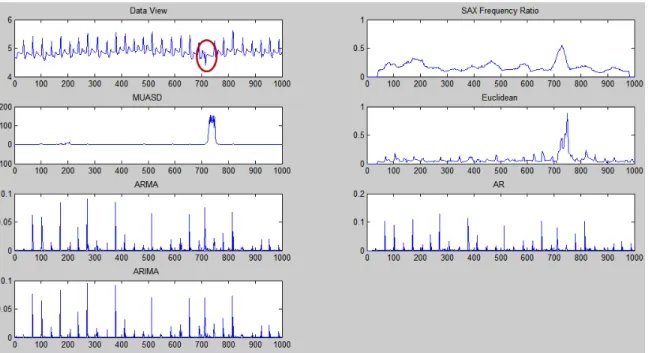
6.3 Proposed Method - Multiple Measure Based Abnormal Subsequence De-tection Algorithm(MUASD) . . . 97
6.3.1 Finding Nearest Neighbor by Early Abandoning . . . 100
6.3.2 Finding Abnormal Subsequence Based on Ratio of Frequencies (SAXFR) . . . 101
6.3.3 Multiple Measure Based Abnormal Subsequence Detection Algo-rithm (MUASD) . . . 106 6.4 Experiments . . . 107 6.4.1 Competing Algorithms . . . 107 6.4.2 Data sets . . . 108 6.4.3 Results . . . 113 6.5 Conclusions . . . 114
7 Conclusions and Future Works 115 7.1 Conclusions . . . 115
7.2 Future Work . . . 117
7.2.1 Rank Based Time Series Anomaly Detection . . . 118
7.2.2 Clustering Based Anomalous Time Series Detection Approach . . 118
7.2.3 Time Complexity of Online Detection Algorithms . . . 118
7.2.4 Anomalous Multivariate Time Series Detection . . . 119
7.2.5 Time Series Data Issues . . . 119
References 120
A Experiments for Rank Based Detection Algorithm 131
B Experiments for Algorithms Based on Clustering and Weighted Ranks 139
in SAXFR 151 C.1 Data set: SYN0 . . . 151 C.2 Data set: ECG1 . . . 156 C.3 Data set: ECG2 . . . 161
L
IST OF
T
ABLES
1.1 Outlier Problems and Corresponding Data sets . . . 6
3.1 Summary of LOF,COF, INFLO, DBCOD, RBDA, RADA, ODMR , ODMRS, ODMRW, and ODMRD for all experiments. . . 55
4.1 Distance Measures Pros and Cons . . . 61
4.2 Correlation coefficient matrix between distances of each pair of series of 30 data sets correspondingly based on different measure. . . 62
4.3 Summary of all time series sets. Similarity of normal series represents that how similar normal series look like to each other. . . 73
4.4 Summary of all time series sets (Cont). . . 74
4.5 RankPowers of algorithms for 47 data sets. . . 82
5.1 Performance of all algorithms. . . 92
5.2 Running time of NMUDIM and average computation workload compari-son between NMUDIM and OMUDIM. . . 93
6.1 SAXFR performances versus length of subsequence . . . 105
6.2 Time series data sets details. . . 109
A.1 Comparison of LOF, COF, INFLO and RBDA for k = 4, 5, 6 and 7 respec-tively for synthetic dataset 1. The highest values are marked as bold. . . 132
A.2 Comparison of LOF, COF, INFLO and RBDA for k = 25, 35 and 50 re-spectively for synthetic dataset 2. The highest values are marked as bold. . . 133
respectively for the Ionosphere dataset. The highest values are marked as
bold. . . 134
A.4 Comparison of LOF, COF, INFLO and RBDA fork = 11, 15, 19, and 22 respectively for the Wisconsin Breast Cancer data. The highest values are marked as bold. . . 135
A.5 Comparison of LOF, COF, INFLO and RBDA for k = 5, 7 and 10 respec-tively for the Iris dataset. The highest values are marked as bold. . . 136
A.6 Comparison of LOF, COF, INFLO and RBDA for k = 7 and 15, respec-tively, for the Iris data with planted anomalies. The highest values are marked as bold. . . 136
A.7 Comparison of LOF, COF, INFLO and RBDA fork = 18, 25, and 35, re-spectively, for the Ionosphere data with planted anomalies. The highest values are marked as bold. . . 137
A.8 Comparison of LOF, COF, INFLO and RBDA for k = 22, 35, and 45, re-spectively, for the Wisconsin Breast data with planted anomalies. The high-est values are marked as bold. . . 138
B.1 Performance of all algorithms for synthetic dataset 2. . . 140
B.2 Performance of all algorithms for synthetic dataset 2 (Cont). . . 141
B.3 Performance of all algorithms for iris with rare class. . . 142
B.4 Performance of all algorithms for iris with rare class (Cont). . . 143
B.5 Performance of all algorithms for ionosphere dataset with rare class. . . 144
B.6 Performance of all algorithms for ionosphere dataset with rare class (Cont). 145 B.7 Comparison of all algorithms for the Wisconsin dataset with rare class. . . . 146
B.8 Comparison of all algorithms for the iris dataset with planted outliers. . . . 147
B.9 Comparison of all algorithms for the ionosphere dataset with planted out-liers. . . 148
B.10 Comparison of all algorithms for the ionosphere dataset with planted out-liers (Cont). . . 149 B.11 Comparison of all algorithms for the Wisconsin dataset with planted
out-liers (Cont). . . 150
1.1 A case that DB(pct, dmin)-outlier definition and distance-based method
doesn’t work. . . 3
1.2 Illustration of a case that density-based algorithm would not work. . . 4
1.3 Outliers and a static data set . . . 6
1.4 Illustration of contextual abnormal subsequence. . . 7
1.5 Examples of anomalous time series . . . 7
2.1 Illustration of reachability distance. . . 20
2.2 A case in which LOF fails for outlier detection. . . 22
2.3 Illustration of SBN and SBT. . . 23
2.4 RNN and Influence Space . . . 24
2.5 Rank in social network . . . 26
2.6 Rank-based Detection Algorithm . . . 27
2.7 Illustration of ranks . . . 28
2.8 Illustration of a case that density-based algorithm would not work. . . 29
2.9 How rank works. . . 30
2.10 A Synthetic dataset with clusters obtained by placing all points uniformly with varying degrees of densities. . . 33
2.11 Synthetic data set 2 . . . 34
2.12 Why LOF does not work. . . 35
3.1 Illustrations ofdk(p),Nk(p)andRNk(p)fork = 3. . . 44
3.2 An example to illustrate ‘Cluster Density Effect’ on RBDA; RBDA assigns
larger outlierness measure to B. . . 47
3.3 Assignment of weights in different clusters and modified-rank. . . 49
3.4 Overall performance of algorithms for 7 data sets. . . 54
4.1 Stock prices for some oil and gas companies and an outlier series. . . 59
4.2 Solenoid current measurements on Marotta MPV-41 series valves. . . 59
4.3 Illustrations for three key measures of MUDIM . . . 66
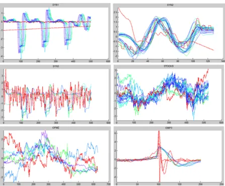
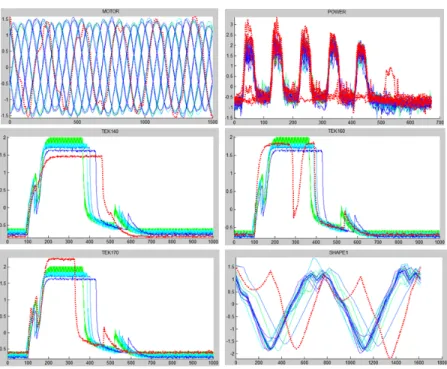
4.4 Typical time series problems . . . 72
4.5 Plots of time series data set, part 1 . . . 75
4.6 Plots of time series data set, part 2 . . . 76
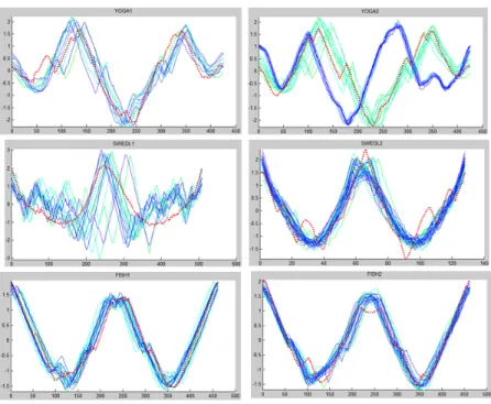
4.7 Plots of time series data set, part 3 . . . 76
4.8 Plots of time series data set, part 4 . . . 77
4.9 Plots of time series data set, part 5 . . . 77
4.10 Plots of time series data set, part 6 . . . 78
4.11 Plots of time series data set, part 7 . . . 78
4.12 Plots of time series data set, part 8 . . . 79
5.1 Experimental data sets . . . 90
5.2 NMUDIM anomaly scores for each data set . . . 91
6.1 Examples for abnormal subsequences. . . 98
6.2 Illustration for sliding window concept. . . 98
6.3 Illustration for reordering early abandoning. . . 101
6.4 Frequency of abnormal subsequence is very low. . . 103
6.5 Experimental results for SYN0 . . . 109
6.6 Experimental results for ECG1 . . . 110
6.7 Experimental results for ECG2 . . . 110
6.8 Experimental results for TEK140 . . . 111
6.10 Experimental results for TEK170 . . . 112
6.11 Experimental results for VIDEOS1 . . . 112
6.12 Experimental results for VIDEOS2 . . . 113
C.1 Synthetic data set SYN0 . . . 151
C.2 SAXFR results for SYN0 . . . 152
C.3 SAXFR results for SYN0 . . . 152
C.4 SAXFR results for SYN0 . . . 152
C.5 SAXFR results for SYN0 . . . 153
C.6 SAXFR results for SYN0 . . . 153
C.7 SAXFR results for SYN0 . . . 153
C.8 SAXFR results for SYN0 . . . 154
C.9 SAXFR results for SYN0 . . . 154
C.10 SAXFR results for SYN0 . . . 154
C.11 SAXFR results for SYN0 . . . 155
C.12 SAXFR results for SYN0 . . . 155
C.13 SAXFR results for SYN0 . . . 155
C.14 Synthetic data set ECG1 . . . 156
C.15 SAXFR results for ECG1 . . . 156
C.16 SAXFR results for ECG1 . . . 157
C.17 SAXFR results for ECG1 . . . 157
C.18 SAXFR results for ECG1 . . . 157
C.19 SAXFR results for ECG1 . . . 158
C.20 SAXFR results for ECG1 . . . 158
C.21 SAXFR results for ECG1 . . . 158
C.22 SAXFR results for ECG1 . . . 159
C.23 SAXFR results for ECG1 . . . 159
C.24 SAXFR results for ECG1 . . . 159
C.25 SAXFR results for ECG1 . . . 160
C.26 SAXFR results for ECG1 . . . 160
C.27 Synthetic data set ECG2 . . . 161
C.28 SAXFR results for ECG2 . . . 161
C.29 SAXFR results for ECG2 . . . 162
C.30 SAXFR results for ECG2 . . . 162
C.31 SAXFR results for ECG2 . . . 162
C.32 SAXFR results for ECG2 . . . 163
C.33 SAXFR results for ECG2 . . . 163
C.34 SAXFR results for ECG2 . . . 163
C.35 SAXFR results for ECG2 . . . 164
C.36 SAXFR results for ECG2 . . . 164
C.37 SAXFR results for ECG2 . . . 164
C.38 SAXFR results for ECG2 . . . 165
C.39 SAXFR results for ECG2 . . . 165
C
HAPTER
1
I
NTRODUCTION
1.1
What are outliers?
Outlier detection techniques attempt to find the objects that are “different" from the rest of the data objects in a given data set. Usually, outliers are generated from certain sys-tem mechanisms that are very different from the syssys-tem mechanism of the rest of data set. The problem of outlier detection is of considerable importance, arising frequently in many different domains such as fraud detection, cyber-intrusion detection, medical anomaly de-tection, image processing and textual anomaly detection [11]. In financial area, banks spend millions of dollars on detecting credit card fraud and money laundering; using out-lier detection techniques, they wish to identify abnormal usage patterns as soon as possible in order to prevent the future loss. In cyber-intrusion field, companies use outlier detec-tion techniques to identify a hacker’s attacks by analyzing the computer or website log files, and then attempt to identify abnormal user behaviors. In image processing, users can take advantage of outlier detection algorithms to identify the image consisting of different objects.
Many researchers have attempted to describe an anomalous object in a given data set. For example, Hawkins [29] suggests that "An outlier is an observation that deviates so
2
much from other observations as to arouse suspicion that is was generated by a different mechanism". Similarly, Chandolaet al. [11] say that "Anomalies are patterns in data that do not conform to a well defined notion of normal behavior". But in real-world applications, a well defined normal behavior sometimes is hard to identify and it may also dynamically change. For instance, a normal user’s behavior on a computer may not be the same as another normal user’s behavior, and all behaviors can change along the time: in the spring semester, students spend more time on preparing homework, document editing, research, whereas in the summer, they spend more time on movies, online games and so on.
Knorr and Ng [43] use very specific approach to define an outlier as "An objectpin a data setDis aDB(pct, dmin)-outlier if at leastpctpercent of the objects inDlie greater than distancedminfromp." This definition is a typical definition for distance-based outlier detection algorithms, but it doesn’t capture all kinds of outliers. For instance, in Figure 1.1, if the object ‘a’ is considered as an DB(pct, dmin)-outlier then according to this definition all objects in cluster C2 are also considered as DB(pct, dmin)-outliers, which is counter intuitive; since object ‘a’ looks more suspicious than all objects in cluster C2.
To overcome the deficiency of the above definition, Breuniget al.[5] suggest to use lo-cal outlier factor (LOF) to capture the degree of an outlier, which is essentially the average of the ratio of the local reachability density of an object and those of the object’sknearest neighbors (kNN). The value of LOF indicates the degree of the oulierness of an object; LOF > 1 generally indicates that the object is an outlier, whereas if LOF is1 or less than the object is a non-outlier. LOF is also one of density-based outlier detection algorithms. Tang et al.[59] obtain the connectivity-based outlier factor (COF) to capture the outlierness of an object. Jinet al.[36] assign to each object the degree of being influenced outlierness (IN-FLO) and introduce a new idea called ‘reverse neighbors’ of a data point when estimating its density distribution. The common theme among these algorithms is that they all assign outlierness to each object in the data set and an object will be considered as an outlier if its outlierness is greater than a pre-defined threshold (usually the threshold is determined by
Fig. 1.1: A case that DB(pct, dmin)-outlier definition and distance-based method doesn’t work. - There are two different clusters C1 and C2, and one isolated data object ‘a’ in this data set. The distance from object ‘b’ to its nearest neighbor,d2, is larger thand1,
the distance from object ‘a’ to its nearest neighbor, which makes ‘a’ unable to be identified.
users or domain experts). The density-based definition seems to work better, but it also has deficiencies. For example, if an outlier has neighbors from different density clusters, then its outlierness is measured incorrectly, as seen in Figure 1.2.
So, in order to capture the real anomalousness of a true outlier, more precise and rea-sonable definitions and algorithms for outlier detection are developed in this dissertation.
This chapter is organized as follows: Section 1.2 introduces the types of outliers and Section 1.3 shows our general goals. Sections 1.4, 1.5 and 1.6 present existing point outliers detection techniques, time series outlier detection techniques and existing online detection techniques respectively.
1.2
Types of Outliers Detection Problems
There are many outlier problems in real world applications; Chandola et al. [11] group them into three categories:
4
Fig. 1.2: Illustration of a case that density-based algorithm would not work. - Red dash circles contain thek nearest neighborhood of ‘A’ and ‘B’ whenk=7.
• Point outliers – Individual data objects that are distinct with respect to the rest of data set.
• Contextual outliers– If data objects are considered as anomalous in a specific con-text but not in other situations, then they are called concon-textual outliers.
• Collective outliers– If a set of data objects is considered as anomalous with respect to the entire data set, then members of the set are called collective outliers.
These three types cover many types of outliers, however, they cannot precisely cover all. The types of data set must be first introduced. Based on data set’s characteristics, there are two types of datasets: set of static data points and time series dataset. The key difference between these two types is time stamp. Both are multi-dimensional; both have dependencies but in time series the same feature is time stamp.
• Static data set simply means a collection of data objects (real-valued) without any time feature or any order by time. In other words, in static dataset the data set doesn’t
change with time. Static dataset could be multivariate (multiple attributes) or univari-ate (single attribute).
• Time series data set represents a collection of data objects with time feature or or-dered by timestamps. In this dissertation, we only consider real-valued time series.
In this thesis, we address three specific types of outlier detection problems.
• Point Outliers Detection. For static data set, point outlier detection is our focus. Note that a data set may contain more than one outlier. For example, in Figure 1.3, data objects "A, B, C and D" are considered as point outliers since they are not in any cluster and are far away from the majority of the data objects. So they are different from the rest of data objects using the ‘neighborhood’ aspect. Point outliers detec-tion has attracted much attendetec-tion in practical applicadetec-tions such as detecting criminal activities, fraud detection, and exceptional cases. In these areas, rare cases may be more interesting and meaningful than normal cases.
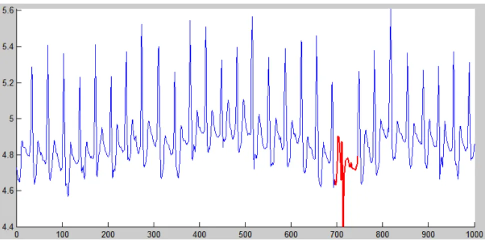
• Contextual Abnormal Subsequence Detection. If a collection of data objects of a series is considered as anomalous with respect to the entire single series, then it is called contextual abnormal subsequence. This anomaly is for a time series data set. For instance, in Figure 6.4, the subsequence highlighted by red is obviously anoma-lous compared with all other subsequences in the series. For contextual abnormal subsequences, we are more interested in detecting the positions of anomalies as soon as possible. Contextual abnormal subsequence detection is a very interesting prob-lem for detecting hacker attacks for computers, or detecting a premature ventricular contraction (PVC) in ECG (electrocardiograms) series.
• Anomalous Series Detection (Collective Outliers). If a single time series is anoma-lous with respect to the other series in a given data set, then it is called an anomaanoma-lous
6
Fig. 1.3: Outliers and a static data set - Data point "A,B,C and D" are outliers with respect to the rest of data objects in this two dimensional data set.
Table 1.1: Outlier Problems and Corresponding Data sets Outlier Types Data set Types Point Outliers Static Contextual Abnormal Subsequences Time Series
Anomalous Series Time Series
series. Anomalous series may also contain point outliers and contextual abnormal subsequences. Two anomalous series are shown in Figure 1.5. Anomalous series detection can be applied for detecting unusual patterns or special events within time series data set such as detecting financial fraud in credit card dataset [23], and detect-ing light curves’ outliers within astronomical data [53].
Fig. 1.4: Illustration of contextual abnormal subsequence. - A subset of ECG data. Red line represents abnormal signal sequence.
Fig. 1.5: Examples of anomalous time series- Red dash represents anomalous series. (Left) Anomalous time series with abnormal subsequences, red circles show the abnormal subsequences. (Right) Another example of anomalous time series.
8
1.3
Our Goals
Our main research will focus on the three outlier detection problems just discussed and our goal is to develop algorithms which have the following characteristics:
1. Normal behaviors have to be dynamically defined. No prior training data set or reference data set for normal behavior is needed.
2. Outliers can be effectively detected even if the distribution of data is unknown.
3. Be adaptive. It can be applied or modified for outlier detection in different domains.
4. Less domain knowledge required of users.
By following above targets, we propose a series of rank based algorithms including rank based detection algorithms, clustering and rank based detection algorithms, multiple measures based anomalous series detection algorithms, and its extended version for online detection. We also propose an algorithm for abnormal subsequence detection.
.
1.4
Point Outlier Detection for Static data set
Point outliers in the static data set usually have abnormal attributes with respect to the rest of data set. Formally, given a data setD, p∈ D, our goal is to findO(p), outlierness ofp, for each object andOthreshold, such that ifO(p)≥Othreshold, thenpis an outlier, otherwise not.
For static dataset, the most important task is to identify one or more individual anoma-lies within a given data set. For example, in Figure 1.3, four isolated data points "A,B,C and D" are far away from the rest of data points, hence, are point outliers.
Unlike supervised data mining techniques, outlier detection is typically an unsuper-vised learning problem because the behaviors or patterns of outliers are unknown. In some
real world application domains, algorithms may need domain expert’s help to decide the optimized parameters, but in most cases this is not possible. Thus, practical applications require outlier detection techniques to make as few assumptions as possible and have to be adaptive to the varieties of anomalies.
1.4.1
Existing Approaches
In recent decades, researchers have proposed different approaches to detect anomalies. Statistics-based approaches (see [30, 51]) were first used for outlier detection based on the assumption that the distributions of datasets are known, e.g., Gaussian distribution or Uniform distribution. A data point was defined as an outlier if it deviates from the existing distribution over a threshold such as three standard deviations. With sufficient knowledge about the dataset, statistics-based methods work effectively. But in the real world, distribu-tions of the data are unknown or arbitrary, significantly impacting the performance of such methods. To overcome this obstacle, clustering-based algorithms have been proposed to detect outliers [27, 69]. The basic idea is that a data point is an outlier if it does not be-long to any cluster. First, these methods build up the clusters by using different algorithms and criteria, then outliers can be found by removing all points that belong to clusters. The effectiveness of this approach depends on the clustering algorithm. Unfortunately, most clustering algorithms are designed for detecting clusters instead of outliers, so the selection performances varies for different data sets.
Knorr and Ng [43] propose to detect an outlier based on its distances from neighboring data points; many other variations of distance-based approaches have been discussed in the literature[19, 20, 70]. The main deficiency found in distance-based approaches is the assumption that the distance from an outlier to its neighbors exceeds the distance from a non-outlier to its neighbors, which is not always true. For example, in Figure 1.1, there are two clusters C1 and C2 of different size. The distance from object ‘b’ to its neighboring objects is apparently greater than the distance from ‘a’ to its neighboring objects which
10
leads to a wrong conclusion that ‘b’ is more suspicious of an outlier than ‘a’. Obviously, ‘a’ is more suspicious of an outlier than ‘b’ since ‘a’ is far away from all its neighbors and ‘b’ is closer to its neighbors. The closeness cannot be simply measured by distance alone.
In order to overcome the deficiencies of distance-based methods, Breunig et al. [5] proposed that each data point of the given data set should be assigned a degree of outlier-ness. In their view, as in other recent studies, a data point’s degree of outlierness should be measured relative to its neighbors; hence they refer to it as the “local outlier factor" (LOF) of the data point. Tanget al.[59] argued that an outlier doesn’t always have to be of lower density and lower density is not a necessary condition to be an outlier. They modified LOF to obtain the “connectivity-based outlier factor" (COF) which they argued is more effec-tive when a cluster and a neighboring outlier have similar neighborhood densities. Local density is generally measured in terms ofknearest neighbors; LOF and COF both exploit properties associated withk nearest neighbors of a given object in the data set. However, it is possible that an outlier lies in a location between objects from a sparse and a denser cluster. To account for such possibilities, Jin et al. [36] proposed another modification, called INFLO, which is based on a symmetric neighborhood relationship. That is, their proposed modification considers neighbors and ‘reverse neighbors’ of a data point when estimating its density distribution. Tao and Pi [60] have proposed a density-based clus-tering and outlier detection (DBCOD) algorithm, which also belongs to the density-based algorithms.
These density-based outlier detection algorithms, such as LOF, COF and INFLO, use the following methodology:
• Define the concept of density of a data point; using the notion of neighborhood (or some variation of it); and
• Calculate the “outlierness” of an object; usually defined as the ratio of a data point’s density with the density in the region surrounding the data point.
1.4.2
Drawbacks in Density-based Approaches
Density-based methodology that exploits k-neighborhood of a data point has many good features. For instance, it is independent of the distribution of the data and is capable of detecting isolated objects. However it also has some shortcomings:
• Density-based algorithms assume that all neighborhoods of a data point have similar density. If some neighbors of the point are located in one cluster, and the other neighbors are located in another cluster and the two clusters have different densities, then comparing the density of the data point with all of its neighbors may lead to a wrong conclusion and the recognition of real outliers may fail, an example is shown in Figure 1.2.
• The notion of density does not work well for sparse data sets such as a cluster of points on a single straight line. Even if each point in the set has equal distances between itself with its closest neighbors, it may still have different density depending on its position in the dataset.
1.4.3
Our Solution
Before proposing a solution for anomaly detection problem, let us consider a concrete ex-ample. Consider the case where a financial institution wishes to find anomalous behavior of its customers. It is obvious that all normal customers are not alike – depending upon their needs and nature all have different ‘normal’ behavior. Individuals with multiple ac-counts and large investments tend to have deposit and withdrawal patterns much different compared to the individuals with small amounts. Consequently, collection of data associ-ated with allusers is likely to form multiple clusters with variable number of data points in each cluster, variable densities, etc. In this data set no two clusters look alike, although they consist of ‘normal’ behavior.
12
data so that in the transformed space all data points have the same statistical distributions. In this dissertation we have attempted to achieve this goal via ‘ranks’ and ‘modified ranks’. In using rank based approach (especially local to the object of interest) we manage to diminish the effect of inter-object distances; and in using ‘modified-ranks’ we diminish the effect of the size of the local cluster(s).
We propose several new approaches [31, 32] for outlier detection, based on a ranking measure and clustering that focuses on the question of whether a point is “interior" for its nearest neighbors. Using our methods, low cumulative rank implies the point is central. For instance, a point centrally located in a cluster has a relatively low cumulative sum of ranks because it is among the nearest neighbors of its own closest neighbors; however a point at the periphery of a cluster has a high cumulative sum of ranks because its nearest neighbors are closer to each other than the point. Use of ranks eliminates the problem of density calculation in the neighborhood of the point, and this improves performance. Our method performs better than several density-based methods, on some synthetic data set as well as on some real data set. More details will be discussed in the following chapters.
1.4.4
Our Contributions
We have implemented novel algorithms based on ranks. Although based on distance, ranks work better than distance and our method captures the anomalousness of an object more precisely in most cases; and it can be applied in broad practical domains.
Rank based clustering algorithm can be used for detecting tight and sparse clusters easily using only one parameter. Based on ranks, it forms clusters with higher accuracy. By combining it with ranks, we show that better performance can be achieved than most of algorithms we have compared with.
1.5
Outlier Detection for Time Series Data Sets
Anomalous series detection and contextual abnormal subsequence detection are both ap-plicable for time series data set. In the current research, only real-valued time series are considered, categorical-valued time series are out of the scope of this investigation. Anoma-lous series detection only focuses on identifying anomaAnoma-lous series whereas the contextual abnormal subsequence problem requires that we detect abnormal subsequence within a sin-gle series, and it requires the comparison between subsequences and the rest of the series. The main difference between these two techniques is: the first one tries to find out which series is anomalous while the latter one tries to find out when abnormal behaviors occur.
These two problems are far more complicated than the algorithms for point outlier detection because of the following challenges:
• Historical information of a series must be considered, but how to summarize the useful historical information is a tough problem.
• Defining a “normal series" is difficult. Since the data in each time series is changing with time, so a normal series att= 1may become anomalous att= 2which makes finding normal series more difficult.
• The behavior of outliers is different for different applications, and it makes detecting abnormal behavior a tough task.
• The noise in the normal series may also cause misleading answers.
• Even in a single application domain, the outlier is also changing with time, so it requires any effective algorithms or techniques to be very adaptive and flexible to deal with dynamic detection. The algorithm must be sensitive to dynamically changing outliers.
14
On-line detection is another important problem. When time series data is huge, getting useful results in a short time using large amount of data is really a big challenge.
These are challenging problems that researchers have to deal with. In the last decade, researchers have proposed different procedures to deal with these issues. Precise problem definitions and associated existing techniques will be discussed in the following sections, along with a brief introduction to our approaches.
1.5.1
Anomalous Time Series Detection
Anomalous time series detection, or outlier time series detection, is an important task in data mining for time series data set, especially for detecting unusual patterns or special events within time series data set Examples include detecting financial fraud in credit card dataset [23], detecting light curves’ outliers within astronomical data [53], and detecting shape anomalies [47] [62].
The problem can be formulated as follows. Given a time series data setD ={xi(t)|1≤
t≤n;i= 1,2, . . . , m}, wherexi(t)represents the data object of theith time series at time
t, nis the length of series and mis the number of time series in the dataset, the goal is to find the outlierness of a series xi, O(xi), and the thresholdOthreshold such that ifxi is an anomalous series, thenO(xi)≥Othreshold; otherwise not. GivenD, the algorithms should be able to calculate the O(xi) and Othreshold for D automatically. Here, the meaning of “difference" between anomalous series and normal series is determined by Othreshold, and it may change from one domain to another, in other wordsOthreshold should not be a fixed value, instead, it needs to be dynamically adjusted for different domains. For example, a threshold to detect a hacker’s attacks is obviously different from a threshold to detect a shape anomaly. Sometimes, the same external cause may result in abrupt changes in most of the time series being considered, e.g., increases in stock prices of most defense contractors as a result of an announcement of impending military conflict. This should not be considered as a case of one time series being anomalous with respect to other time
series. The algorithm should able to distinguish this from real anomalous series.
1.5.1.1 Existing Approaches
In recent years, researchers have used many ideas to find an anomalous time series. Leng, et al. [44], use a new time series representation method, based on key points and dynamic time warping to find the anomalous series. Fujimakiet al.[25] construct a global AR model for all series and then measure the anomaly score at timetas the gap between the observed value and the predicted value. Keogh and Ratanamahatana [38] propose a lower bound based pruning method for dynamic time warping to detect anomalous series. Protopapas et al. [53] uses cross-correlation as the measure of similarity between two individual light curves and use the average correlation as outlier measure. Yankov et al. [68] propose fastk-nearest neighbor and early abandon to find the unusual time series for a time series database. Discrete Wavelet Transform [8], and Discrete Fourier Transform [21] also can be applied for anomalous series detection by calculating the distance between coefficients of transformed series.
1.5.1.2 Issues and Our Solution
To the best of our knowledge, most of existing methods for anomaly detection relies on a single measure; however, in general, any individual measure fails to capture varieties of anomalies which may occur in multiple application domains. We propose an anomaly detection method based on a combination of multiple distance measures (MUDIM) [34] where strengths lies in the properties that several types of anomalies can be captured by it.
1.5.1.3 Our Contributions
We show that our multiple distance measures based methods do better than single distance measure based method and it can capture a variety of anomalous series without requiring more domain knowledge. Rank-based algorithms are applied to adjust the weights of
dif-16
ferent features. The most interesting advantage of it is that in our approach the weights change automatically, based on anomalousness of each distance feature; other algorithms do not achieve the same goal in the same conditions.
1.5.2
Abnormal Subsequences Detection in a Single Series
This problem can be formulated as follows. Suppose X = {x(t)|1 ≤ t ≤ n}is a time series wherex(t)represents the value of the seriesX at timetandnis the length ofX. A subsequence ofXis defined asXp,m ={x(p), ..., x(p+m−1)|1≤p ≤n−m+ 1; 1<
m ≤ n}. The goal is to find an abnormal subsequenceXp,m such that outlierness ofXp,m exceeds a specified threshold. An abnormal subsequence is also known as “discord" in other literatures [41, 6, 13].
1.5.2.1 Existing Approaches
To detect any abnormal subsequence in a series many solutions have been proposed. Lin et al. [45] uses SAX, suffix tree and non-self match to find unusual medical time series discords such as ECG (electrocardiograms) data set. ECGs are time series that measure the electrical activities of the heart, and a premature ventricular contraction (PVC) is a relatively common cardiac arrhythmia that can be easily detected in ECG compared with a normal heart beat by a cardiologist. The techniques for anomalous time series detection can be applied here to help cardiologists to identify the status of patient’s heart.
Keogh et al. use ‘ heuristic discord discovery’ based on augmented tries for detecting discord [37, 41]. Fu et al. [13] and Bu et al. [6] both suggest a method based on haar wavelet transformation to find the best alphabet size and word size to further improve speed of their time series discord detection algorithm by pruning unnecessary calculations.
1.5.2.2 Our Solutions
We proposed a novel outlier detection method based on sliding window and multiple dis-tance measures. The method achieves better performance than the existing methods in a variety of datasets used in our experiments.
Our algorithm can detect all abnormal subsequences within a single series with only one parameter, w, the length of subsequence. Unlike otherkNN based methods, it is able to detect all abnormal subsequences even when k similar subsequences exist in a single series, whereas other methods may fail.
1.6
Online (Real-time) Anomalous Series Detection
Online detection requires detecting the anomalous series as soon as possible. So the algo-rithms for online detection must be very effective and efficient.
1.6.1
Related Research
This problem has been studied by various researchers [67, 63, 40, 61, 56, 9, 41].
Yamanishi, et al. [67], address this problem using a probability-based model in non-stationary time series data. Wei, et al. [63], use frequencies of symbolic aggregation representation (SAX) of time series. Keogh,et al., [40, 41] employ suffix tree comparison, HOT SAX algorithm, and nearest non-self match distance. Toshniwal, et al., [61] extend HOT SAX algorithm to detect outliers in streaming data time series. Sadik, et al. [56], develop an algorithm based on adaptive probability density functions and distance-based techniques to detect outliers in the data streams. Xie and Tang [65] propose a new dynamic hidden semi-Markov model to detect time-variant user behavior.
Unfortunately, some of the above online methods can only be applied for detecting outliers in a single series. In contrast with the above methods, our focus is on the impor-tant variation where multiple time series are being observed simultaneously, and detection
18
should occur as soon as one (or more) series begins to differ from the rest. In our approach no training set is required and no model is constructeda priori. Some methods mentioned earlier, such as [63, 56], can be used directly for online detection. Other methods, proposed by Chandolaet al. [10], such as anomalous series detection with training data sets based using kNN, window based, predictive model based, segment based methods, can also be adapted for online detection. But the main problems found in these methods are:
• Finding the optimal values of parameters of the algorithms requires the user to have expert domain knowledge which may not be available.
• High amount of computational effort is required, so that these methods are not suit-able for online detection in large data streams.
• Concept drifting ( the statistical properties of data objects change over time) and data uncertainty are common problems in data streams, which prevent successful application of fixed model based methods.
1.6.2
Our Solutions
To overcome these problems, we propose online algorithms [33] that utilize information from multiple distance metrics. These unsupervised methods require only one parame-ter, viz., the number of nearest neighbors (k). Experimental results show that our ap-proaches are successful in anomalous time series detection, and also computationally effi-cient enough to permit online execution. Our online algorithms have higher accuracy and works better in more data sets than other competing methods.
C
HAPTER
2
P
OINT
O
UTLIERS
D
ETECTION
B
ASED
O
N
R
ANKS
The goal for point outliers detection algorithms is to find the point outliers that are “differ-ent" from the rest of the data points in a given data set. Practical applications concerning outlier detection occur in many domains such as fraud detection, cyber-intrusion detection, medical anomaly detection, image processing and textual anomaly detection [11].
As mentioned in the first chapter, density-based algorithms seem to work better in most of the application domains, so we will first review typical density-based algorithms in de-tail. This chapter is organized as follows: in Section 2.1 we review the density based ap-proaches of anomaly detection algorithms. Then in Section 2.2 we introduce our algorithm - RBDA, and finally show the experiment results in Section 2.3.
2.1
Review of Density-based Approaches
In density based approaches the main idea is to consider the behaviors of a point with respect to its neighbors. The neighborhood is conceptualized by considering k nearest neighbors, wherekis either iteratively estimated or is a preassigned integer. The underlying
20
assumption is that if density of a pointpis ‘different’ than densities of its neighbors, it must be an anomaly. The main difference between the approaches described below is in how they define the local behavior related with density.
2.1.1
LOF (Local Outlier Factor) approach
Breuniget al.[5] proposed the following approach to find an outlier. For each pointpin the given dataset, they evaluate its “local outlier factor" (LOF); a point whose LOF is ‘large’ is declared anomalous.
Fig. 2.1: Illustration of reachability distance. - reach −distk(p1, o) and reach −
distk(p2, o)fork=4. This figure is from Breunig [5]
1. Find the distance,dk(p), betweenp and itskth nearest neighbor. The distance can be any measure; but here the Euclidean distance is used. Denote the set ofknearest neighbors ofpbyNk(p) = {q∈D− {p}: d(p, q)≤dk(p)}.
3. The average reachability distance is
reach−distavg(p) =
P
q∈Nk(p)reach−distk(p, q)
|Nk(p)|
.
The local reachability density of a point is defined as the reciprocal of reachability distance
`k(p) = [reach−distavg(p)]−1.
4. Finally, this local reachability density is compared with the local reachability densi-ties of all points inNk(p), and the ratio is defined as LOF (local outlier factor):
Lk(p) = [ P o∈Nk(p) `k(o) `k(p) |Nk(p)| ].
5. The LOF of each point is calculated, and points are sorted in decreasing order of
Lk(p). If the LOF values are ‘large’, the corresponding points are declared as out-liers.
6. To account fork, the final decision is taken as follows: Lk(p)is calculated for se-lected values ofkin a pre-specified range, max Lk(p)is retained, and apwith large LOF is declared an outlier.
LOF performs well in many application domains, but its effectiveness will diminish if the density of an outlier is close to densities of its neighbors. In Figure 2.2, data objecto1 is isolated but its density is very close to densities of objects inC1which makes LOF fail to detect this outlier.
2.1.2
COF (Connectivity-based Outlier Factor) approach
To solve the deficiency found in the LOF, Tanget al.[58] suggest a new method to calculate the density as described below. Define the distance between two non-empty setsP andQ
22
Fig. 2.2:A case in which LOF fails for outlier detection. - (This figure is from Tanget al.[58])
as d(P, Q) = min{d(p, q) : p ∈ P, q ∈ Q}. This can be used to define the minimum distance between a point and a set by treating the point as a singleton set.
1. As in the previous algorithm, letNk(p)be the set ofknearest neighbors ofp.
2. Define set-based path (SBN) of lengthk as a path< p1, p2, . . . , pk >based on the set{p,Nk(p)} such that for all 1 ≤ i ≤ k −1, pi+1 is the nearest neighbor of the
set{p1, p2, . . . , pi}in{pi+1, pi+2, . . . , pk}. In other words, the SBN-path represents the order in which nearest neighbors ofpare successively obtained. In simple words, SBN is an ordered list of all neighbors ofp.
3. The Set-based trail (SBT) is an ordered collection ofk −1edges associated with a given SBN path< p1, p2, . . . , pk >. Theith edgeeiconnects a pointo∈ {p1, . . . , pi} topi+1 and is of minimum distance; i.e., length ofei is equal to
d(o, pi+1) = d({p1, . . . , pi},{pi+1, . . . , pk}). Denote the length of edge asdist(ei). Figure 2.3 illustrates these concepts.
4. Givenp, the associated SBN path< p ≡p1, p2, . . . , pk>, and the SBT< e1, e2, . . . , ek−1 >,
the weightwi for edgeei is proportional to the order in which it is added to SBT set. Then the average-chaining distance (A) ofp is the weighted sum of the lengths of
Fig. 2.3: Illustration of SBN and SBT. - The objectp’sk-nearest-neighbors are q1, q2,
and q3 when k = 3. Then SBN path from pis {p, q1, q3, q2}, and SBT is <e1, e2, e3> respectively.
the edges. That is:
ANk(p)(p) = k−1 X i=1 wi×dist(ei). where wi = 2(k−i) k(k−1)
5. Finally, the connectivity-based outlier factor (COF) of a pointpis defined as the ratio ofp’s average-chaining distance with the average of average-chaining distances of its
knearest neighbors; COFk(p) = [ANk(p)(p)][ P o∈Nk(p)ANk(p)(o) |Nk(p)| ]−1.
6. As in LOF, larger values of COFk(p)indicates thatpis an outlier with higher possi-bility.
24
COF works better than LOF in the data sets with sparse neighborhoods (such as a straight line), but its computation cost is larger than LOF.
2.1.3
INFLO (INFLuential measure of Outlierness by symmetric
relationship) approach
Proposed by Jinet al.[36], in INFLO theknearest neighbors and reverse nearest neighbors of an objectpare used to obtain a measure of outlierness.
Fig. 2.4:RNN and Influence Space - Fork=3,Nk(q5)is{q1, q2, q3}. Nk(q1)={p, q2, q4}.
Nk(q2) = {p, q1, q3}. Nk(q3)= {q1, q2, q5}. RNk(q5) = {q3, q4}. The original figure is
from Jinet al.[36].
1. Reverse Nearest Neighborhood (RNN) of an objectpis defined as
RNk(p) ={q : q∈Dandp∈ Nk(q)}.
instances, it may be empty, because for allq∈ Nk(p),pmay not be in any of the set ofNk(q).
2. Thek-influential space forp, denoted as ISk(p) =Nk(p)∪ RNk(p).
3. The influential outlierness of a pointpis defined as
INFLOk(p) = 1 den(p) P o∈ISk(p)den(o) |(ISk(p))| where den(p) = d1 k(p).
Thus for anyp, INFLO expands Nk(p)to ISk and compares p’s density with average density of objects in ISk. By using the reverse neighborhood, INFLO enhances its ability to identify the outliers in more complex situation, but it’s performance is poor if an object
p’s neighborhood includes data objects from groups of different densities, then outlierness ofpcannot be correctly measured.
2.2
Rank-Based Detection Algorithm (RBDA)
We present a new approach to identify outliers based on mutual closeness of a data point and its neighbors. The key idea of our algorithms is to use rank instead of distance. The idea of rank is borrowed from social network. Detecting outliers in a given data set resembles finding the most unpopular person in a given social network. Consider the social network in Figure 2.5: if we want to find if Bob is an unsocial person in it, then simply ask him this question:“who are your best friends?", then ask all “friends" of Bob the same question, if Bob is not in the list of his friends, he might be unpopular. Summaries of all answers are able to give a more clear conclusion about who unsocial person is. For example, in Figure 2.5 (a), Bob says that Eric is his closest friend but Eric says Bob is not one of his best friends. We ask the same question for every person in this social network. For example, the same questions for Eric and Jack show that they are best friends to each other. It can
26
be seen that Bob will appear to be No.1 unsocial person in this illustration. If we use the concept of ranks to capture the relationship of ‘the best friend’, then we can also use it to capture the outlierness of an outlier.
Fig. 2.5: Rank in social network- Rank can be used to measure popularity in a social network.
To understand mutual closeness considerp ∈ D andq ∈ Nk(p). That is, consider a q which is “close” top because it belongs tok-neighborhood ofp. In return, we ask “how close isptoq?". Ifpandqare ‘close’ to each other, then we argue that (with respect to each other)pandq are not anomalous data points. However, ifqis a neighbor ofpbutpis not a neighbor ofq, then with respect toq,pis an anomalous point. Ifpis an anomalous point
with respect to most of its neighbors, thenp should be declared to be an anomaly. When measuring the outlierness of p, instead of distance, we use the ranks calculated based on neighborhood relationships betweenpandNk(p)in our outlier detection algorithms. This forms the basis of RBDA [31].
2.2.1
Description of Rank-based Detection Algorithm (RBDA)
Al-gorithm
28
Fig. 2.7: Illustration of ranks- Red dash shows kNN ofp when k is 3 and long blue dash shows a circle with radius ofd(p, q3)and center ofq3. ThekNN ofpis {q1,q2, q3}. Then rq3(p)=4, because d(q3, p) is greater than any of d(q3, q3), d(q3, q4), d(q3, q1) and
d(q3, q5).
1. Letp∈ Dwhere|D| = n, Nk(p)denotes the set of its k-neighbors,N(p), denotes all the neighbors ofp ∈ D, it is defined as N(p) = {d(p, o);p 6= o, o ∈ D}. Let
rq(p) denote the rank of p with respect to q, and it is defined as rq(p)=|I| where
I = {d(q, o);d(q, o) < d(p, q), d(q, o) ∈ N(q)}. For all q ∈ Nk(p), calculate the
rq(p).
2. ’Outlierness’ ofp, denoted byOk(p), is defined as:
Ok(p) =
P
q∈Nk(p)rq(p)
|Nk(p)| . (2.1)
IfOk(p)is ‘large’ thenpis considered an outlier.
3. One criterion to determine ‘largeness’ is described below. LetDo={p∈D| Ok(p)≤
O∗}whereO∗ is chosen such that the size ofD
size ofD. We normalizeOk(p)as follows: Lk(p) = ln(Ok(p)) (2.2) Zk(p) = 1 Sk (Lk(p)−L¯k) (2.3) where ¯ Lk = 1 |Do| X p∈D Lk(p)andSk2 = 1 |Do| −1 X p∈D (Lk(p)−L¯k)2
and if the normalized valueZk(p)is ≥2.5, then we declare that pis an outlier. In this criterion we have assumed that the distribution of Zk(p) = S1
k(Lk(p)−
¯
Lk) (normalized for mean and standard deviation) will be approximated by the standard normal random variable and P(Zk(p) = S1
k(Lk(p)−
¯
Lk) > 2.5) ≈ 0.006. Hence, value ofZk(p) = S1k(Lk(p)−L¯k)>2.5will be an outlier.
2.2.2
Why does RBDA work?
Fig. 2.8: Illustration of a case that density-based algorithm would not work. - Red dash circles contain thek nearest neighborhoods of ‘A’ and ‘B’ whenk=7.
30
Fig. 2.9: How rank works. - Red dotted circle represents thek nearest neighborhood of ‘A’ when k is 7; Blue solid circle shows the range of I when calculating ranks of ‘A’ for each itskNN. The number of data objects in blue circle represents the rank of ‘A’ with respect to the object in the center of the circle. (Left) Ranks for ‘A’; (Right) Ranks for ‘B’
Before explaining why RBDA works, first we examine a scenario in which the density-based algorithm would fail. Consider the data set in Figure 2.8. There are three groups of data objects and one isolated data object - ‘A’. Data object ‘B’ is from group3. When
k is 7, thek nearest neighbors of both ‘A’ and ‘B’ contain the data objects from different density groups. In this case, the density-based outlier detection algorithm, LOF, assigns a higher outlierness value 1.5122 to ‘B’ and lower outlierness value 1.1477 to ‘A’ which is counter intuition. Density-based algorithms assume that all the neighbors of interested data objects are from the same density groups, but such is not the case in our example. In this illustration, LOF also suffers the same deficiency whenkis 6, 7, or 8.
To overcome this issue, instead of focusing on the calculation of density, RBDA chooses another approach: using ranks instead of distance. Although rank is calculated based on distance, it contains more useful information. The basic idea is that if an object is an outlier, its rank with respect to itskNN is larger, whereas a normal object’s rank is smaller.
Since RBDA requires calculating the ranks of the interested data object with respect to itskneighborhood, an object far away from many data objects in the data set will have
large rank. For example, in Figure 2.9, object ‘C’ is the 7th nearest neighbor of object ‘A’, but ‘A’ is the 31st neighbor of ‘C’, because ‘C’ is more close to the center of data set than ‘A’. Thus in Figure 2.9, RBDA outlierness (average rank) of ‘A’ is 10 and that of ‘B’ is less (6.5714) as expected.
2.3
Experiments:
We use two synthetic and three real datasets to compare the performance of RBDA with LOF, COF and INFLO. Metrics to compare the algorithms are described below.
2.3.1
Metrics for Measurement
To evaluate the performance of the algorithms, three metrics were selected – precision, recall, and Rank-Power [2, 49, 57, 7].
Suppose the setDofnobjects containsdttrue outliers. Suppose, using a given outlier detection algorithm, we identifymmost suspicious instances inD. Letmtbe the number of true outliers amongminstances. ThenPrecision, which measures the proportion of true outliers in topmsuspicious instances, is:
Pr= mt
m,
andRewhich measure the accuracy of an algorithm is:
Re= |mt|
|dt|
.
Precision and recall are insufficient to capture complete effectiveness of an algorithm. One algorithm may identify an outlier as the most suspicious while another algorithm may iden-tify it as the least suspicious. Yet the values for the above two measures remain the same. Ideally, an algorithm will be considered more effective if the true outliers occupy top
po-32
sitions and non-outliers are among the least suspicious instances. “RankPower" was pro-posed by Tang et al. [58] to capture this notion. Let Ri denote the rank of the ith true outlier. Then,
RP= mt(mt+ 1) 2Pmt
i=1Ri
.
Rank-Power takes maximum value 1 when allntrue outliers are in topnpositions.
For a fixed value of m, larger values of all three of these metrics imply better perfor-mance.
2.3.2
Synthetic Datasets
Two synthetic datasets, shown in Figures 2.10 and 2.11, are used to evaluate the outlier detection algorithms. For illustrative convenience, we use only 2-dimensional data points so that outliers can be seen easily. In each dataset, there are multiple clusters with different densities. In each dataset, we have placed six additional objects, (A, B, C, D, E, and F) in the vicinities of the clusters to evaluate their ‘outlierness’ by LOF, COF, INFLO, and our proposed algorithm, RBDA.
In tables below, we summarize the performance of the algorithms, Pr represents preci-sion, Re represents recall, and RP represents Rank-Power.
2.3.2.1 Synthetic Dataset 1
Synthetic dataset 1 contains four clusters of different densities consisting of 36, 8, 8, and 16 instances. Four different values ofk and four values ofmare used; results are shown in Table A.1 in Appendix.
Fork = 4, only COF and RBDA algorithms find all six outliers within topmranked instances, and their RankPowers are higher than those of LOF and INFLO algorithms.
Fork =5, 6, and 7 RBDA has higher precision and recall than the other algorithms; and RBDA is the only algorithm that obtains the maximum RankPower of 1 for everym.
Fig. 2.10: A Synthetic dataset with clusters obtained by placing all points uniformly with varying degrees of densities.
-2.3.2.2 Synthetic Data set 2
Synthetic dataset 2 consists of 515 data objects including six planted outliers; this data set has one large normally-distributed cluster and two small uniform clusters.
Results are presented in Table A.2 in Appendix for k = 25,35, and 50, and m = 5,10,15,20and 30. It can be seen that for k =25 and 35, RBDA has the best precision, recall and Rank-Power for all m from 5 to 30. When k is increased to 50, RBDA still performs better than others except form= 20. The reason why LOF doesn’t work fork=50 is shown in Figure 2.12: the true outliero has shorter distance to itskth nearest neighbor than objectq. When comparing the ratios of densities,q’s value is larger thano so that it makesqlook more like an outlier thano.
In this experiment, RBDA algorithm works better than others in most of the cases, and fork = 25 and 35, it achieves the best performance.
34
Fig. 2.11: Synthetic data set 2- A synthetic data set with one cluster obtained using the Gaussian distribution and other clusters by placing points uniformly.
Fig. 2.12: Why LOF does not work. - Red dash circle encloses thek nearest neighbors (kNN) of objectowhich is an outlier, and blue circle representskNN of objectqwhenkis 50.
36
2.3.3
Real Datasets:
We have used three well known datasets, namely the Iris, Ionosphere, and Wisconsin breast cancer datasets. We use two ways to evaluate the effectiveness and accuracy of outlier detection algorithms; (i) detect rare classes within the datasets, rare classes are generated by removing a majority of objects from the original class (this methodology has also been used by other researchers such as Feng et al. and Tang et al. [22, 58]) and (ii) plant outliers into the real datasets (according to problem specific knowledge) and expect outlier detection algorithms to identify them.
2.3.4
Real Datasets with Rare Classes
In this subsection, we compare the algorithms in detecting rare classes. A class is made ‘rare’ by removing most of its observations. In all cases, the value ofk is chosen between 5% to 10% percentage of the size of the dataset. Because the attributes are dependent, Mahalanobis distance is used to measure the distance between two points.
2.3.4.1 Iris Dataset
This well-known data set contains the categorization of iris flowers to three classes: Iris Setosa, Iris Versicolour, Iris Virginica, with 50 instances each. The Iris Setosa class is linearly separable from the other two classes, but the other two classes are not linearly separable from each other. We randomly remove 45 instances from Iris Setosa class to make it ‘rare’; the remaining 105 instances are used in the final dataset. Three selected values ofkare 5, 7, 10. In Appendix, Table A.5 summarizes our findings.
We observe that fork = 5, LOF and RBDA both have the highest precision and recall values while RBDA has the best RankPower for all values ofm; COF performs poorly (its precision and recall values are all zero). The reason for COF’s poor performance is that instances of rare class are close to each other which decrease average-chaining distance of
COF algorithm significantly and thus decrease its usefulness.
Fork = 7, LOF performs better than RBDA. In particular, COF doesn’t find any outlier within top 10 ranked instances.
Fork = 10and all values ofm, LOF, INFLO and RBDA perform well.
2.3.4.2 Johns Hopkins University Ionosphere Dataset
The Johns Hopkins University Ionosphere dataset contains 351 data objects with 34 at-tributes; all attributes are normalized in the range of 0 and 1. There are two classes labeled as good and bad with 225 and 126 data objects respectively. There are no duplicate data objects in the dataset. To form the rare class, 116 data objects from the bad class are ran-domly removed. The final dataset has only 235 data objects with 225 good and 10 bad data objects. Four values ofk = 11, 15, 20 and 23 are used; values ofmare assigned at 5, 15, 30, 60 and 85. Results are presented in Appendix Table A.3.
We observe that, for k = 11, among all algorithms RBDA has the best precision, re-call and RankPower except for m = 15. LOF and INFLO algorithms achieve the best RankPower form = 15; but RBDA is the only algorithm that finds all ten ‘bad’ class in-stances.
Fork = 15, LOF has higher RankPower than RBDA for m= 15 and 30; but for other values ofm, RBDA is the winner and has largest values of RankPower. RBDA algorithm finds all 10 ’bad’ class instances while other algorithms only find 9 of them whenmis less than 85. Fork = 20 and 23, situation is very similar to the previous case.
In general, RBDA shows the best overall performance.
2.3.4.3 Wisconsin Diagnostic Breast Cancer Dataset
Wisconsin diagnostic breast cancer dataset contains 699 instances with 9 attributes. There are many duplicate instances and instances with missing attribute values. After removing all duplicate instances and instances with missing attribute values, 236 instances labeled
38
as benign class and 236 instances as malignant were left. Following the method proposed by Cao [7], 226 malignant instances are randomly removed. In our experiments the final dataset consisted 213 benign instances and 10 malignant instances. Results are presented in Appendix Table A.4.
For k = 11, RBDA achieves the best precision and recall for m = 15, 20 and 50, and gets the best RankPower form= 30 and 40. COF has the best precision and recall form= 30, 40 and 50, and it also has the best RankPower form= 15, 20 and 50.
For k = 15, 19 and 22, the relative performance results are similar. Either RBDA or COF gets the best precision, recall and RankPower for every m. But none of them can achieve the best performance for all values ofm.
In general, COF performs a little better than RBDA, but for certain values ofm, RBDA has better RankPower than COF.
2.3.5
Real Datasets with Planted Outliers
In experiments described in this subsection we plant some outliers into the real datasets according to datasets’ domain knowledge.
2.3.5.1 IRIS with Outliers
We insert three outliers into IRIS dataset, that is, there are three classes with 50 instances each and 3 planted outliers. The first outlier has maximum attribute values, second outlier has minimum attribute values, and the third has two attributes with maximum values and the other two with minimum values. Appendix Table A.6 contains the results for this setting.
Fork = 7 andm ≥ 10, all algorithms found the three outliers, but their RankPowers are different. RankPower of COF is lower than those of the other three algorithms; LOF, INFLO and RBDA all have the best performance for precision, recall and RankPower.
Fork = 15, INFLO and RBDA are the best because they all rank three outliers in top three positions which are exactly the expected results that outlier detection algorithms are
designed to do. LOF and COF have the worst Rank-Power.
2.3.5.2 Johns Hopkins University Ionosphere Dataset with Outliers
For ionosphere dataset, two classes labeled as good and bad, with 225 and 126 instances respectively, are kept in the resulting dataset. Three outliers are inserted into the dataset; the first two outliers have maximum or minimum value in every attribute, and the third has 9 attributes with unexpected values and 25 attributes with maximum or minimum values. The unexpected value here is a value that is valid (between minimum and maximum) but is never observed in real datasets1.
In Appendix Table A.7, we observe that RBDA consistently performs better than the other algorithms. For all values ofkandm, RBDA achieves the best precision, recall and RankPower. In addition, RBDA algorithm is the only algorithm that detects all three rare class instances for all threekvalues whenmis 40.
The gap of performance between RBDA and other algorithms is large since RBDA’s RankPower is almost twice that of other algorithms, for everykandm. The overall perfor-mance of RBDA is the best.
2.3.5.3 Wisconsin Diagnostic Breast Cancer with Outliers
After removal of duplicate instances and instances with missing attribute values, only 449 instances were left with 213 instances labeled as benign and 236 as malignant. Two out-liers were planted into dataset. Both outout-liers have maximum or minimum values for all attributes.
In Appendix Table A.8, for everyk, our algorithm, RBDA, is the only algorithm that has the maximum RankPower (1) for every value ofm. It also has the best precision and recall for allk andm. We can observe that even the maximum RankPower of LOF, COF
1For example, one attribute may have a range from 0 to 100, but the value of 12 never appears in real