Cholesky-factorized sparse Kernel in support vector machines

Title: Cholesky-Factorized Sparse Kernel in Support Vector Machines

Author: Alhasan Abdellatif

Advisors: Jordi Castro, Lluís A. Belanche

Departments: Department of Statistics and Operations Research and

Department of Computer Science

Academic year: 2018-2019

Master of Science in

Advanced Mathematics and

Mathematical Engineering

Universitat Polit`ecnica de Catalunya

Facultat de Matem`

atiques i Estad´ıstica

Master in Advanced Mathematics and Mathematical Engineering

Master’s thesis

Cholesky-Factorized Sparse Kernel in

Support Vector Machines

Alhasan Abdellatif

Supervised by Jordi Castro and Llu´ıs A. Belanche

June, 2019

I would like to express my gratitude to my supervisors Jordi Castro and Llu´ıs A. Belanche for the continuous support, guidance and advice they gave me during working on the project and writing the thesis. The enthusiasm and dedication they show have pushed me forward and will always be an inspiration for me. I am forever grateful to my family who have always been there for me. They have encouraged me to pursue my passion and seek my own destiny. This journey would not have been possible without their support and love.

Abstract

Support Vector Machine (SVM) is one of the most powerful machine learning algorithms due to its convex optimization formulation and handling non-linear classification. However, one of its main drawbacks is the long time it takes to train large data sets. This limitation is often aroused when applying non-linear kernels (e.g. RBF Kernel) which are usually required to obtain better separation for linearly inseparable data sets. In this thesis, we study an approach that aims to speed-up the training time by combining both the better performance of RBF kernels and fast training by a linear solver, LIBLINEAR. The approach uses an RBF kernel with a sparse matrix which is factorized using Cholesky decomposition. The method is tested on large artificial and real data sets and compared to the standard RBF and linear kernels where both the accuracy and training time are reported. For most data sets, the result shows a huge training time reduction, over 90%, whilst maintaining the accuracy.

Keywords

Contents

1 Introduction 3

2 Background 4

2.1 Support Vector Machines . . . 4

2.2 Support Vector Machines Solvers . . . 9

2.3 Compactly-Supported RBF Kernel . . . 10

2.4 Cholesky Decomposition . . . 10

3 Sparse Kernel Properties 11

4 Literature Review 12

5 Method 13

6 Results and Discussion 16

7 Conclusion 20

References 21

A Proof of Theorem 5.3 23

1. Introduction

Classification in machine learning is a problem of assigning certain labels to patterns using a pre-labeled training set. Support Vector Machine (SVM) is a supervised learning model used to perform tasks such as classification. It can be considered one of the most powerful machine learning algorithms due to several properties including that it is formulated as a convex optimization problem so a global minimum is guaranteed, it can adapt to non-linear problems using the kernel trick which uses non-linear kernels to map points into a feature space, and it is memory efficient as it uses a subset of the data points called support vectors. In addition, it is one of the leading models in text and document categorization.

However one of the main limitations of using SVM is that it does not scale up well to large data sets as its time complexity is O(m3_{) [5], where m is the number of the training points. Hence, solving}

the associated optimization problem with very large data sets can be computationally expensive. Several solvers have been developed to solve the optimization problem associated with SVM including LIBSVM library which has a time complexity between O(n×m2) and O(n×m3) [4], where n is the dimension of the training points, and LIBLINEAR library [20] which is practically much faster than LIBSVM [6] but can work only with a linear kernel which is a disadvantage, since it is often required to better separate the data in high-dimensional feature space using non-linear kernels (e.g. RBF Kernel).

Many contributions have been made to speed up SVM classification for large data sets. One idea is to perform a preprocessing step on the large data set to obtain a smaller but yet well-representing subset. The smaller subset is then supplied directly to an SVM solver which takes much shorter time compared to training on the whole large data set. For example, in [21], they performed two steps to reduce the training set: a data cleaning based on a bootstrap sampling and algorithm to extract informative patterns. In [13], a data compression technique based on Learning Vector Quantization (LVQ) neural network is tested on large training sets and in [10] an algorithm for instance selection is developed especially for multi-class problems and is based on clustering. However, one drawback of these approaches is that removing some data points from the training set can often result in an underfitting model that performs poorly on the original data set. Another idea is to replace the RBF kernel by an approximate one, which is much faster to compute, and hence training the data set can take less time. The experiments in [8] show that the approximate kernel can be more than 30 times faster than the exact RBF kernel. In [9], they substitute the RBF kernel by a kernel with a sparse matrix into the dual formulation of the optimization problem, in which they achieve a time reduction of nearly 47% while the accuracy is preserved. While replacing the RBF kernel by an approximate or a sparse RBF kernel can offer a time reduction, these approaches used non-linear solvers (e.g. LIBSVM) which are relatively slow.

In this thesis, we study an approach that speeds-up SVM training combining both the better sepa-ration by non-linear kernels and the faster training by a linear solver, LIBLINEAR. The approach uses a compactly-supported RBF kernel which have been studied and used in [9] and [3]. Its associated sparse gram matrix is factorized, using Cholesky decomposition, into a lower triangular matrix which acts as the mapped training points in the feature space. The matrix is then fed into LIBLINEAR, to solve the primal optimization problem associated with SVM. The the dual variables are then computed to classify new test points. To verify our approach, it is tested against many real data sets and an artificial data set of large sizes. The training time and test accuracy are reported and compared to the ones obtained using LIBSVM with RBF Kernel and LIBLINEAR with a linear kernel.

The remainder of the thesis is organized as follows: an overview of SVM classification is provided in section 2.1 and some known SVM solvers are discussed in section 2.2. In section 2.3, the compactly-supported RBF kernel is discussed and some of its properties are highlighted in section 3. In section 4 some related literature results are shown. Our method is then explained discussing both training and the testing procedures in section 5. The results of the approach are presented and compared to other methods in section 6. Finally, a conclusion is drawn pointing out both the benefits and limitations of the approach in section 7.

2. Background

In this section, we point out some basics behind SVM including the hard and soft margin problems, the use of the kernel trick, the primal and dual formulations and multi-class classification. We then review some popular SVM solvers and their main applications. The sparse kernel used in the approach is introduced and finally we discuss Cholesky factorization and the approximate minimum degree permutation algorithm. In the discussion below, consider m as the number of training points andn as the number of features.

2.1 Support Vector Machines

Support Vector Machine (SVM) is a machine learning algorithm that was first introduced by Vapnik in 1963 [23] and further developed in 1995 [5]. It tries to find a hyperplane that best separates the data points into two different classes. The hyperplane is then used to classify new points to either of the two classes. One method to obtain such hyperplane is to maximize the separation between the two classes, this separation is called a margin. Any hyperplane can be written as

wTx−b = 0 (1)

where w ∈ _Rn _{is the normal vector to the hyperplane, x ∈}

Rn any point satisfying the hyperplane and

Figure 1: Margin between two classes in SVM, adapted from [12].

b ∈_Ris the intercept.

Consider binary-classes data points xi ∈ Rn and their labels yi ∈ {1,−1} ∀i = 1 ...m, the method

depicted in Figure 1.

Lemma 2.1.1The margin between two parallel hyperplanes wTx−b=a1 and wTx−b=a2 is |a_k1−_wa_k2|.

Proof. Consider a pointx1 lies on the first hyperplane and a point x2 lies on the second, then x2 can be

written asx2 =x1+αw. Then we have

wTx2 =wTx1+αwTw

a2+b =a1+b+αkwk2

α= a2−a1

kwk2 .

The margin between the hyperplanes iskαwk which is

kαwk=|α|kwk= a2−a1

kwk2 kwk=

|a1−a2|

kwk .

From Lemma 2.1.1, it can be deduced that the margin between the two hyperplanes wTx −b = 1 and wTx−b = −1 is _kw2_k. Since maximizing _kw2_k is equivalent to minimizing 1₂kwk2_{, the optimization}

problem associated with SVM can be formulated as min w,b 1 2kwk 2 ₍₂₎ Subject to yi(wTxi−b)≥1∀i = 1 ...m (3)

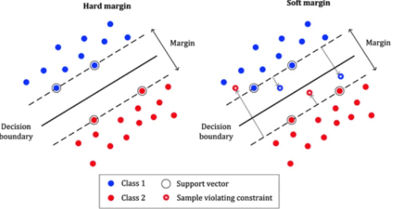
The above optimization problem is calledhard margin SVM and only works with data sets that are linearly separable, i.e., there exists a hyperplane that can separate all labeled points into the two classes with no point lies in the incorrect side of the margin. Another formulation was developed called soft margin that allows each data point xi to have a corresponding error ξi ≥ 0 such that points with ξi > 0 lie in the

incorrect side. The difference between the hard and soft margins is shown in Figure 2. The soft margin

optimization problem can be formulated as following min w,b,~ξ 1 2kwk 2_+C m X i=1 ξi (4) Subject to yi(wTxi −b)≥1 +ξi (5) ξi ≥0 ∀i = 1 ...m (6)

where C > 0 is a hyper-parameter that represents the trade-off between the training error and margin maximization. In order to classify a new data point, z → {1,−1}, we use the following rule

z →sgn(wTz−b), (7)

wheresgn(x) is the sign function. The above methods work with data points in the input space, another method was developed in [5] uses what so-calledkernel trick which maps the data points from the input space to a high dimensional feature space allowing better separation for linearly inseparable data points. The method seeks to find a mapping function

φ:Rn→RN, (8)

whereNis the dimension of the feature space, such that the new feature space provides a better separation, however it is not clear how we define the mapping φ.

It turns out that the kernel function defined by

k(xi,xj) =φ(xi)Tφ(xj) (9)

appears directly in the dual formulation of the soft margin optimization problem with no need to compute the mappingφ(x) if we knowk(xi,xj) beforehand. The kernel functionk(xi,xj) is associated with a gram

matrixK whereKij =φ(xi)Tφ(xj) which can be written as

K =BBT, (10)

whereB is an (m×N) matrix and each row represents a data point mapped in the feature space. When

φis the identity function,k is often called a linear kernel in which casek(xi,xj) =xiTxj andB will be the

originalm×n data points matrix. Several non-linear kernels have been developed such as the Radial Basis Function (RBF) kernel

krbf(x,y) = exp (−

kx−yk2

2σ2 ) (11)

and polynomial kernel

kpol(x,y) = (xTy+c)d, (12)

wherec,d andσ are parameters to be tuned. In our method, we focus only on the RBF kernel. In order to derive the dual formulation, we use Wolfe Duality.

Theorem. 2.1.2 ( Wolfe Duality) If f(x),h(x)and g(x) are convex and differentiable functions in the primal problem

min

x f(x) (13)

Subject to h(x) = 0 (14)

then a sufficient and necessary condition for the optimality of the dual function q(λ,µ) =min

x L(x,λ,µ)

is

∇xL(x,λ,µ) = 0, (16)

where L is the Lagrangian function, λ and µ are the dual variables associated with the constraints (14) and (15), respectively.

The dual problem of of (13) can then be written as max

x,λ,µ L(x,λ,µ) =f(x) +λ

T_{h(x) +µ}T_{g(x) (17)}

Subject to ∇xL(x,λ,µ) = 0 (18)

µ≥0. (19)

Since the objective function (4) and the constraints (5) and (6) are convex and differentiable functions, the Wolfe duality can be used. The Lagrangian function of the soft margin problem (4), usingφ(x) instead of x, is

L(w,b,ξ,λ,µ) = 1 2w

T_{w +C e}T_ξ+λT_{(−D(Bw−be)−ξ+e)−µ}T_{ξ, (20)}

where λ ∈ _Rm _{and µ ∈}

Rm are the dual variables of the constraints (5) and (6), respectively, D is an

m×m diagonal matrix with the labels of the data points ande ∈Rm is a vector of ones. Then the dual

problem can be written as max w,b,ξ,λ,µ 1 2w T_{w +C e}T_ξ+λT_{(−D(Bw−be)−ξ+e)−µ}T_{ξ (21)} Subject to w −(λTDB)T = 0 (22) λTDe = 0 (23) C e−λ−µ= 0 (24) λ≥0,µ≥0. (25)

Substituting equation (22) in (21) and using equations (23) and (24), we can arrive at the following formulation max λ λ T_e−1 2λ T_DBBT_{Dλ (26)} Subject to λTDe= 0 (27) 0≤λ≤C. (28)

Hence, knowing the kernel matrix K =BBT is enough to solve the SVM dual problem. After solving the last optimization problem and obtaining λ, equation (22) can be used to calculate the weights

w = m X i=1 λiyiφ(xi) (29) =BTDλ. (30)

In order to calculate the interceptb, we need to find a pointxk which is a support vector, such point will

have ξk = 0 and 0< λk <C. Usingyk(wTφ(xk)−b) = 1, we get

b=wTφ(xk)− 1 yk (31) = m X i=1 λiyik(xi,xk)−yk. (32)

To classify a new pointz using the dual formulation we use

z →sgn(wTφ(z)−b) = sgn(

m

X

i=1

λiyik(xi,z)−b). (33)

To perform multi-classification, two common methods are one-vs-rest and one-vs-one. In our work, we focus on one-vs-rest method which trains k classifiers, where k is the number of classes in the data set. For each classifier, one class is labeled by 1 and the rest by −1 and we assign to a new pointz the label that maximizes the decision function

z →argmax j=1...k ( m X i=1 λj_iyik(xi,z)−bj). (34)

Before the sparse kernel is introduced, some properties of kernels are listed below.

Theorem. 2.1.3 Let xi ∈ Rn,∀i = 1, ... ,m, then a symmetric function k(x,y) is a kernel if and only if

the matrix

K = (k(xi,xj))i,j=1,...,m

is positive semidefinite.

Proof. Proving the forward direction, letk(x,y) be a kernel and using equation (9), then for any non-zero vector v ∈_Rm_{, we have} vTKv = m X i,j=1,...,m vivjKij = m X i,j=1,...,m vivjhφ(xi),φ(xj)i =h m X i=1 viφ(xi), m X j=1 vjφ(xj)i =k m X i=1 viφ(xi)k2≥0

which proves that K is positive semidefnite. To prove the reverse direction, It is enough to prove the following result on positive semidefinite matrices: If K is positive semidefinite matrix, then it can be written as K =BBT for some real matrix B.

This result can be proved by observing thatK is a symmetric diagonalizable matrix and thus can be written as K =QΛQT, where Q is an orthogonal matrix and Λ is a diagonal matrix. Let B =Q√Λ, then

BBT =Q√Λ√ΛQT =QΛQT =K and this completes the proof.

Lemma 2.1.4 The multiplication of two kernels is also a kernel.

Proof. Let A and B be kernels and let (C)ij = (A)ij(B)ij, this is known as Hadamard product and is

denoted byC =A◦B. Using eigendecomposition, we can write A=XαiaiaiT B =XβjbjbTj . Then we have A◦B =X ij αiβj(aiaiT)◦(bjbTj ) =X ij αiβj(ai◦bj)(ai ◦bj)T.

Since (ai◦bj)(ai◦bj)T is positive semidefinite andαiβj ≥0 for anyi,j, thenA◦B is positive semidefinite

and henceC is a kernel using Theorem 2.1.3.

2.2 Support Vector Machines Solvers

Many libraries have been developed to solve the optimization problems associated with support vector machines, such as SVMLIGHT, LIBSVM and LIBLINEAR. We consider here LIBSVM and LIBLINEAR libraries. LIBSVM [4] was first developed in 2000 and can work with both a linear kernel and non-linear kernels (e.g RBF kernel). It has a time complexity betweenO(n×m2) andO(n×m3), which can be very slow in case of very large datasets. It uses a decomposition method named Sequential Minimal Optimization (SMO) which was developed in 1998 at Microsoft Research Lab [17]. The method breaks the quadratic optimization problem into small sub-problems which are solved analytically.

On the other hand, LIBLINEAR [20] works only with linear classification problems. It can be very efficient when the number of features is large and it is often much faster than LIBSVM. For example, in [6], they tested both libraries on a data set where the numbers of instances and features are 20, 242 and 47, 236, respectively. LIBLINEAR gave almost the same accuracy as LIBSVM with a training time of about 3 seconds whereas LIBSVM took nearly 346 seconds. LIBLINEAR solves an unconstrained optimization problem of the form:

min w 1 2w T_w+C m X i=1 max(0, 1−yiwTxi), (35)

2.3 Compactly-Supported RBF Kernel

SVM solvers do not store the gram matrix associated with the RBF kernel, instead each entry is directly computed and used in solving the optimization problem. This is because such a matrix is dense and the available storage will not meet its space requirement. Since sparse matrices offer much smaller space requirements and reduction of time complexity, a family of kernels with sparse gram matrices have been studied and used in [9], [3] and [14]. These kernels can be constructed by multiplying the RBF kernel by some compactly-supported radial basis function. We particularly consider the function

kc(x,y) = (1−αkx−yk)l+, (36)

where a+ = max{a, 0}, x,y ∈ Rn and α > 0. R. Askey in [19] proved that kc is positive definite if

l ≥ bn/2c+ 1, whereb.c is the floor function. Satisfying the condition onl,kc can then be regarded as a

kernel function using Theorem 2.1.3.

Applying Lemma 2.1.4, an RBF kernel with a sparse gram matrix can be constructed by multiplying the kernel kc by the RBF kernel:

k(x,y) =kc(x,y)krbf(x,y) (37)

= (1−αkx−yk)l₊exp (−kx−yk

2

2σ2 ). (38)

The parameterαcontrols the kernel sparsity, the percentage of zero elements in the kernel matrix, increas-ingα makes the kernel matrix more sparse. The parameterl affects the smoothness of the kernel function.

2.4 Cholesky Decomposition

The Cholesky decomposition [11] of a real positive definite matrix Ais of the form A=LLT,

whereL is a lower-triangular matrix, called Cholesky factor. The Cholesky factor is unique ifAis positive definite matrix, whereas it needs not be unique if Ais positive semidefinite.

Cholesky decomposition finds many applications in numerical solutions, for example it can be more efficient thanLU factorization in solving a system of linear equations [18]. For large matrixA, computing the Cholesky factor L can be computationally expensive, however if the matrix is sparse, Cholesky factor-ization can be very fast. Several libraries have been developed to perform Cholesky factorfactor-ization including CHOLMOD library [22], which can also perform a sparse Cholesky factorization.

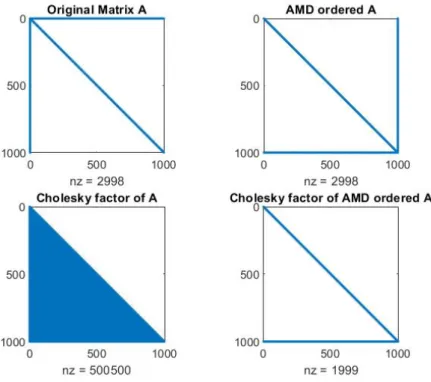
Applying Cholesky decomposition to a sparse matrix does not always guarantee that the Cholesky factor will be as sparse as possible. Several algorithms have been studied to perform a permutation of the rows and columns of the matrix A before applying the Cholesky factorization to increase the sparsity of the Cholesky factor. One common algorithm is the approximate minimum degree [2], which tries to find the best permutationP so that Lis as sparse as possible. In Figure 3, the Cholesky factorization is done on an arrowhead matrix before and after applying the approximate minimum degree algorithm in Matlab (AMD function), it shows that the number of nonzero elements is much smaller in the Cholesky factor when using approximate minimum degree algorithm.

Figure 3: Comparison between Cholesky factors with and without applying AMD function in Matlab.

3. Sparse Kernel Properties

In this section, some properties of the sparse kernel are discussed. Since the choice of the parameters is crucial in training SVM, the limit values of theα parameter are discussed below .

Lemma 3.1 Let K be the gram matrix associated with the kernel k(xi,xj) defined in equation (38),

then

lim

α→0K =Krbf

lim

α→∞K =Im

where Im is an m×m identity matrix and Krbf is the matrix of the RBF kernel.

Proof. Using the expression ofkc(xi,xj), it is clear that for any i,j

lim

α→0(1−αkxi−xjk)

l

+= 1,

which from equation (37) results in limα→0K =Krbf. On the other hand

lim

α→∞kc(xi,xj) =

0 i 6=j 1 i =j since (Krbf)ii = 1∀i = 1 ...mthen limα→∞K =Im.

From Lemma 3.1, we can observe that as we increase α, the sparse kernel matrix K gets sparser. As

α becomes very large the kernel matrix becomes totally distorted as the identity matrix. The sparse kernel follows nearly the same performance as the RBF kernel when α is very small.

Theorem 3.2 : (Gershgorin Circle) Let A be a matrix with entries aij and let Ri =

P

j6=i|aij|. Let

D(aii,Ri) be a closed disk centered at aii with radius Ri. Then every eigenvalues of A lies within at least

one of the Gershgorin disks D(aii,Ri)

Lemma 3.3 The radius of the Gershgorin Disk of matrix of the sparse kernel k defined by (37) is less than that associated with the RBF Kernel.

Proof. Letdij and zij be the entries of the matrices of krbf andkc, respectively. Since the entries of both

matrices are non-negative,dij >0 andzij ≥0, we can drop out the notation of absolute values defined of

radii in Theorem 3.2. We can show that

X j6=i Kij = X j6=i dijzij < X j6=i dij.

if we can prove that,

zij <1 for j 6=i.

Sinceα >0 and l is a positive integer, it is clear thatzij = max{0, (1−αkxi −xjk)l}<1 for j 6=i.

4. Literature Review

In section we review some literature papers that have used the compactly supported kernel in support vector machines. A closely related work was developed in [9], where they used the same sparse kernel in equation (38). They pointed out some properties of the sparse kernel and describe techniques to tune the sparsity parameter α. One technique is to perform a trade-off between similarity A(α) and sparsity S(α), they defineA(α) andS(α) as follows:

A(α) = p hK,KrbfiF

hK,Ki_FhKrbf,KrbfiF

, (39)

wherehK1,K2i_F =Pm_i,j=1K1(xi,xj)K2(xi,xj) is the Frobenius inner product between two matrices and

S(α) = number of zero entries in K

m2 . (40)

The trade-off can be done by maximizing a linear combination between similarity and sparsity, max

α A(α) +βS(α). (41)

whereβ >0 is a tuning parameter. Another procedure is to pre-evaluate the maximum number of nonzero elements that can be stored on the machine and from that we can choose a lower bound of the sparsity. For example, if only 25% of the nonzero entries can be stored, then we may setS(α)≥0.75 and 1/α to

be the first quartile of the pairwise distances kxi−xjk,i,j = 1, ...m.

One application they performed is replacing the matrix of the RBF kernel in the dual problem of SVM, K = BBT in equation (26), by the sparse matrix of the compactly supported RBF kernel. They tested their method on a small data set (100 instances) and reported the accuracy which was very close to the one obtained using the RBF kernel. They also used the sparse kernel in training an LS-SVM classifier, which instead of solving a quadratic optimization problem solves a linear system, and tested that on a relatively larger data set of (5000) where they reported both accuracy and time, in the best case the sparse kernel saved the computation time by 47% while maintaining good accuracy.

In [3], they used the same sparse kernel for regression problems using LS-SVM. They set the parameter

α = 1/3σ, where σ is the same parameter in the RBF kernel. They solved the linear system associated with LS-SVM by using Cholesky factorization. They tested both the compactly-supported kernel and the RBF kernel on a sinc-toy problem with 1334 training points. The compactly-supported kernel obtained a similar accuracy with a speed-up of about 50% compared to the RBF kernel.

While the work done in [9] was able to reduce the training time, they solved the dual optimization problem using non-linear solvers such as LIBSVM which is often slow. Although they did not show results for very large data sets, it is likely that the speed-up by the sparse kernel will not compensate the painful slowness in LIBSVM for very large data sets. In our method, we were able to reach a speed up of over 90% for data sets of more than 100k and 200k instances. In the next section, we dicuss the details of our method.

5. Method

As discussed in section 2.2, LIBLINEAR is much faster than LIBSVM but only works with a linear kernel and hence favours data sets where the linear kernel is enough to best separate the points. On the other hand, whenn is much smaller thanm, non-linear kernels are favoured to get better accuracy in which case LIBSVM is better.

Our approach combines both the better performance of non-linear kernels and the faster training by LIBLINEAR. It seeks to find anm×N matrixB that represents the data points inN-dimensional feature space which best separates the data such thatK =BBT _{, whereK is a non-linear kernel. Having obtained}

B, we can directly feed it to LIBLINEAR, as input matrix, to solve the primal optimization problem. It is not clear however what is the optimal dimensionNof the space in which we can separate the data points.

Definition 5.1 ( Shattered set) Let A be a set and C be a class of sets, we say that C shatters A if for each subset a of A, there is some element c of C such that

a=c ∩A.

In the context of classification, shattering means that for all possible assignments of the labels to the set pointsA, any classifier model c ∈C is able to correctly classify them all.

Definition 5.2 Vapnik–Chervonenkis (VC) dimension of a class of classifier is the maximum number of points the classifiers can shatter.

a VC dimension of 3, meaning that there is a combination of 4 points inR2 such that no straight line can

shatter them, as shown in Figure 4.

Theorem 5.3The VC-dimension of the set of affine classifiers{f :f(x) =sgn(wTx+b),w ∈Rd,b∈R}

is d+ 1.

A proof of Theorem 5.3 can be found in Appendix A. From Theorem 5.3, we can say that any m data points can be shattered inRm using hyperplanes.

In our approach, we choose the dimensionN =m, in which case the matrixB becomes anm×msquare

Figure 4: A line can not shatter this combination of 4 points, adapted from [16]

matrix, although there might be spaces with dimension less than mthat can shatter them points as well. The question becomes how the kernel matrixK can be decomposed intoBBT. One way is to useCholesky decomposition discussed in section 2.4 in that case B becomes a lower triangular matrix, for the sake of simplicity we denote B byL.

Since kernel matrices are in general dense, Cholesky decomposition can be computationally expensive, in addition to the huge space requirements needed to store large matrices associated with large data sets. For example, a data set of m= 200, 000 instances requires at least 160GB, using 8 bytes for every entry, to store the kernel matrix before applying the factorization. In order to overcome the space and time problems, the sparse RBF kernel discussed in section 2.3 is used, where it acts as an approximation for the RBF kernel. The usage of the sparse kernel matrix significantly reduces the storage needed for both the kernel matrix and Cholesky factor. For example, if the sparsity is over 95% for the same 200, 000 instances, we need less than 4GB to store the kernel matrix. In addition, sparse Cholesky factorization algorithm is much faster than the one with a dense matrix.

Although L is a triangular matrix, it is still needed to be sparse because of the space requirement. For this reason, before applying the decomposition, a permutation (P) of the rows and columns of the sparse kernel matrix K was performed by approximate minimum degree algorithm discussed in section 2.4. It is important to note that the permutation for the kernel matrix K is equivalent to the permutation of the rows of L, i.e., it is a reordering of the data points in the matrix L. Hence, before solving the primal optimization problem we need to reorder the labels,yi∀i = 1 ...m, with the same permutationP.

Solving the primal problem using LIBLINEAR yields the weightsw and the interceptb, but noww ∈_Rm

since each data point (each row of the matrix L) is in Rm. To classify a new test point z ∈ Rn, we use

equation (7) :

z →sgn(wTφ(z)−b),

(22) which can be rearranged as

(LTDp)λ=w, (42)

where Dp is a permuted version of the labels diagonal matrix D. The reason that D has to be permuted

is that both L andw are not in the original order but in the permuted order. The linear system ofLTDp

can be very large but yet sparse and triangular which makes it very fast to solve. Then we can use the classification rule (33) z →sgn( m X i=1 λP_i yik(xi,z)−b), (43)

wherek(xi,z) is the sparse kernel, yi andxi are in their original order and λP is aP-permuted version of

λ.

The approach can be viewed as training using the primal problem and testing using the dual variables and is summarized in Algorithm 1.

Algorithm 1Binary Classification using Cholesky-Factorized Compactly Supported Kernel

Input :Data set xi ∈Rn,yi ∈ {1,−1}, Test point z ∈Rn

Output :Class of z

• Choose the parameters α,σ,l andC.

• Compute the sparse matrix of the compactly supported kernel K where Kij = (1−αkxi −xjk)l+exp (−

kxi−xjk2

2σ2 ).

• Apply the approximate minimum degree algorithm to the matrix K to find the permutation matrix P.

• Apply the permutation P to bothK andy to get KP andyP

• Apply the Cholesky factorization to the permuted matrix Kp to obtain the Cholesky factor L.

• Solve the primal optimization problem using LIBLINEAR with matrix Land labels yP and trade-off

parameter C, to get the weights w and intercept b.

• Solve the system (LTDP)λ=w for λ, whereDP is a P-permuted labels diagonal matrix.

• Apply z →sgn(Pm

i=1λPi yik(xi,z)−b), where λp is theP-permuted version ofλ.

In order for the Cholesky factor L to be unique, we need to make sure that the sparse kernel matrix is positive definite, for this reason a diagonal matrix with small entries (0.0001) is added to the sparse kernel matrix. Since the diagonal elements of the kernel matrix is 1, adding such diagonal matrix will not change the main characteristics of the kernel matrix.

When choosing the parameterα, we followed a similar idea proposed in [3] where they set the parameter

α= 1/3σ, whereσ is the same parameter in the RBF kernel. The sparse RBF kernel can then be written as k(x,y) = (1− kx−yk 3σ ) l +exp (− kx−yk2 2σ2 ). (44)

The value of 3σ can be regarded as the cut-off of the pairwise distances such that distances that are greater than 3σ has a correspondingzeroin the RBF kernel which means that points that are very far from each other has a zero similarity. The value ofσ now has the reverse effect ofα as discussed in section 3, decreasingσ will make the kernel matrix sparser. We tried different values ofσ for each data set, hopefully to find the best value that makes the kernel matrix sparse enough and yet gives high test accuracies, details about these values are shown in the next section 6.

The parameterl is set to be the smallest integer satisfyingl ≥ bn/2c+1 in order to satisfy the condition set by Askey in [19] for the positive definiteness of the kernel. In the experiments we performed, we choose the value ofC to be 1. We note thatC can be fine tuned for every data set, though the accuracies obtained using RBF and linear kernels suggested that the value of 1 is good enough.

To perform multi-classification, we used the one-vs-rest method discussed in section 2.1. The corre-sponding modification in Algorithm 1 would be in the last three steps as we obtain k-values of w andb, wherek is the number of classes. The system

(LTDP)λj =wj,∀j = 1, ... ,k (45)

is solved k times and finally we compute the decision function Pm

i=1λ

P,j

i yik(xi,z)−bj for each class

j = 1 ...k and pick the class achieving the maximum decision value.

The implementation of the algorithm is done in Python using scikit-learn [24] libraries which have im-plementation of LIBSVM and LIBLINEAR. The computation of the sparse kernel uses a Cython wrapper so that the comparison could be fair as both LIBSVM and LIBLINEAR in scikit-learn uses Cython wrappers as well. For the sparse Cholesky factorization, CHOLMOD library [22] is used, it also provides the imple-mentation of the approximate minimum degree algorithm. The code of the algorithm is shown in Appendix B and can be accessed on the online repository [1]. The next section shows the results of the approach of the sparse RBF kernel on some data sets and the comparison to RBF and linear kernels.

6. Results and Discussion

To validate our approach, we performed a comparison with the standard RBF kernel using LIBSVM and with the linear kernel using LIBLINEAR. Several data sets are used in the comparison and each one was splitted into training and testing sets. The different methods are trained on the training sets and validated on the test sets. The training time (in seconds) and the testing accuracy are reported and compared for each method.

Since our approach uses a non-linear kernel and a linear solver, we wanted to make sure that it still performs well even when a linear kernel performs poorly. For this reason, we created an artificial data set that is linearly inseparable such that the RBF kernel performs much better on accuracy than the linear kernel. The artificial data set has 3 dimensions and 3 classes and is shown in Figure 5. Other data sets are obtained from online resources [15] and summarized in Table 1.

For each data set, we tried different values ofσ to obtain the best accuracy and to make sure that both the kernel and Cholesky factor matrices are as sparse as possible. Since we are limited with the amount of RAM on the machine, we start with small values of σ and then gradually increase σ and observe the corresponding test accuracy. We choose the best value ofσ that gives the highest accuracy on the test set and still provides a high sparsity such that the matrices can be stored on the machines. The best value of

Figure 5: Swiss-roll artificial data set.

Data sets Train points Test points Features Classes

Artificial1 225000 75000 3 3 Artificial2 100500 49500 3 3 Skin Segmentation 108783 71913 3 2 Covtype 97319 47934 54 2 CodRNA 59535 80890 8 2 Shuttle 43500 14500 9 7 a6a 11220 21341 123 2 usps 7291 2007 256 10

Table 1: Summary of data sets used in the experiments

The comparison of our approach to LIBSVM with RBF kernel and to LIBLINEAR is presented in Table 2, where we also report the sparsity of the kernel matrix and time reduction percentage obtained when using the sparse RBF kernel. The platform used for the experiments was Intel Core i7-3520M dual core 2.9 GHz with 8MB RAM and all the codes were compiled by Python 3.6.7 under a Linux operating system (Ubuntu 18.04.2).

Concerning the first three data sets in Table 2, the linear kernel performed poorly, in terms of accuracy, compared to the RBF kernel and sparse RBF kernel. Moreover, the sparse kernel approach outperforms both the RBF kernel and linear kernel, where the accuracy is very close to that of the RBF kernel but with a huge training time reduction (between 90 and 99%) . For example, the artificial data set with over

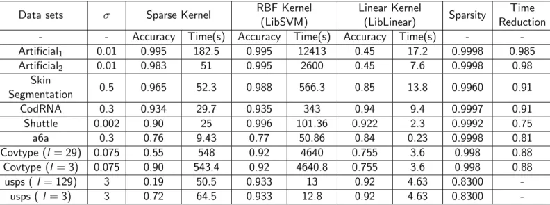
Data sets σ Sparse Kernel RBF Kernel (LibSVM) Linear Kernel (LibLinear) Sparsity Time Reduction - - Accuracy Time(s) Accuracy Time(s) Accuracy Time(s) - -Artificial1 0.01 0.995 182.5 0.995 12413 0.45 17.2 0.9998 0.985 Artificial2 0.01 0.983 51 0.995 2600 0.45 7.6 0.9998 0.98 Skin Segmentation 0.5 0.965 52.3 0.988 566.3 0.85 13.8 0.9960 0.91 CodRNA 0.3 0.934 29.7 0.935 343 0.94 9.4 0.9997 0.91 Shuttle 0.002 0.90 25 0.996 101.36 0.922 2.3 0.9992 0.75 a6a 0.3 0.76 9.43 0.77 50.86 0.84 0.23 0.9998 0.81 Covtype (l = 29) 0.075 0.55 548 0.92 4640 0.755 3.6 0.998 0.88 Covtype (l = 3) 0.075 0.90 543.4 0.92 4640.8 0.755 3.6 0.998 0.88 usps ( l = 129) 3 0.19 50.5 0.933 13 0.92 4.63 0.8300 -usps ( l = 3) 3 0.72 64.5 0.933 12.8 0.92 4.63 0.8300

-Table 2: Comparison of the experimental results using the sparse kernel, RBF kernel and linear kernel

200k instances took around 12,400 seconds using the RBF kernel, whereas the sparse RBF kernel took only 182.5 seconds which is around 68 times faster. When training on the skin data set, our approach was 10 times faster with only 2% reduction in accuracy compared to the RBF kernel. In the CodRNA data set, the accuracies of the three methods are almost the same, while our approach is much faster than the LIBSVM with RBF kernel with 91% time reduction. In the Shuttle data set, the accuracy was dropped by 10% when using the sparse kernel, which can be substantial, but provides faster performance.

In situations where the linear kernel is sufficient (e.g. a6a), LIBLINEAR gave the highest accuracy and the fastest performance as well. In the experiments with the usps and Covtype data set, the accuracy of the sparse kernel was dropped significantly, the reason is the condition set on the parameter l. When the number of features is large, the value of l will also be large as l ≥ bn/2c+ 1 and since the values of kc(x,y) = (1−αkx−yk)l defined in equation (36) is less than one then the values of the sparse RBF

kernel become negligibly small compared to the value of intercept b and thus the decision function, used in equation (43) as g(z) =sgn( m X i=1 λP_i yik(xi,z)−b),

will give most of the time a sign that is determined by the dominant valueb. One way to fix this problem is to reduce the value ofl, although this will violate the condition set by Askey [19] to make sure that matrix is positive definite. However, we note that this condition is a sufficient, not a necessary one. In Covtype and usps data sets, we rerun the experiments with l = 3 , which gave a very good accuracy in Covtype data set, close to that of the RBF kernel with faster training, but failed to give a similar performance in usps data set.

It is worth mentioning that, the second step in Algorithm 1 ( computing the sparse RBF kernel) took most of the training time. Other steps such as Cholesky factorization and solving the linear system are very fast, when the matrices are sparse. The testing time was not reported as we were only concerned with the training performance. It is not also necessary to store the kernel matrix between the training and testing sets, we can compute each entry of the matrix and use it directly when classifying a testing point.

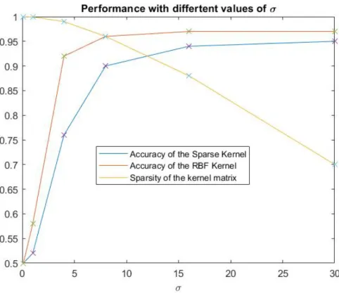
our approach with the sparse RBF kernel might not be a good choice. The large value of σ will produce a dense kernel matrix which in case of very large data sets can not be stored on the machines. In addition, training with the sparse RBF kernel can even be much slower. For instance, we show in Figure 6 different experimental results performed on a small data set, used in [6], named svmguide1 with 3,089 training instances. The accuracies of both our approach and RBF kernel are plotted for different values of σ and we also plot the sparsity of the kernel matrix. We observe that the accuracy increases with the increase of

σ while the sparsity decays. If we decide thatσ = 16 is a good choice which provides an accuracy of 94%, then we will have a sparsity of 0.88 which will not be very good for large data sets.

7. Conclusion

In this thesis, we studied a novel approach of training support vector machines that has shown a signif-icant speed-up over traditional training methods. As discussed in section 2, support vector machines is a classification method used to assign labels to patterns. It builds a model by using a set of pre-labeled training set and solving an optimization problem to find a hyperplane that separates the data points into two classes. One advantage of using SVM is that it can use a kernel trick that maps the data points into high-dimensional features space where it is easier to separate the points.

Working with the non-linear kernels can be computationally expensive and usually solving the SVM optimization problem with them is painfully slow for large data sets. A kernel with sparse matrix was discussed in section 2.3 and we showed some of its properties in section 3. The kernel is constructed by multiplying a compactly- supported radial basis function by the RBF kernel. This multiplication leads to a kernel by using results from Theorem 2.1.3 and Lemma 2.1.4 provided that a condition is met on the parameter l in the kernel definition. Some literature papers have used the same sparse kernel, particularly [9] and [3], in support vector machine problems. One has replaced the RBF kernel by the sparse kernel directly in the optimization problem. Although, such substitution led to a speed-up in the training time, they used non-linear solvers which are still slow in case of large data set. Further results are shown in section 4.

In section 5 we discussed the details of our algorithm. The algorithm tries to combine the better performance of RBF kernel and the faster training of LIBLINEAR [20]. It computes the sparse matrix of RBF kernel discussed in section 2.3 and instead of solving the dual problem, we a perform a Cholesky factorization of the sparse matrix of the constructed RBF kernel. To make sure that the Cholesky factor is sparse as well, to meet space requirements, the approximate minimum degree algorithm [2] is used. The factor matrix, which now represents the data points mapped into the feature space, is then used to solve the primal optimization problem of SVM using LIBLINEAR solver. The novel approach showed very promising results over the standard training with RBF kernel. Experiments were conducted on several data sets and the time reduction obtained was sometimes over 90% while the accuracy was nearly the same as the one obtained using the RBF kernel. In cases where the linear kernel did not perform well, our approach was still able to perform similar to the RBF kernel but with much faster training procedure.

The main limitation of this approach is the need to store the sparse kernel matrix. This limitation can lead to out-of-memory errors if the parameter σ is chosen inappropriately and makes the approach not a good choice if σ has to be large to obtain a high accuracy. Another issue happens when the number of features is large, this will make the parameterl large as well because of Askey’s condition. The large value of l may lead to poor accuracy as discussed in section 6. Reducing the value of l practically enhanced the accuracy but theoretically we are not sure if the function defined in equation (38) will be a kernel in general.

One possible continuation of this work is to solve its limiting situations. One could try to find an alternative relation between the sparsity parameterα and the parameter σ that does not lead to memory problems if σ is large. One could also try to fix situations where the number of features is large either by providing theoretical bounds on the parameter l that guarantee that the function kc is a kernel or by

finding a practical framework that performs well when the number of features is high and still meets the current theories. Another future work is to apply similar ideas on other applications that use the kernel trick such as SVM in regression, kernel PCA and spectral clustering.

References

[1] A. Abdellatif (2019). Master thesis code. GitHub repository, http://www.github.com/ AlhasanAbdellatif123

[2] A. George and W. H. Liu (1989).The evolution of the Minimum Degree Ordering Algorithm. SIAM Review. 31 (1): 1–19.

[3] B. Hamers, J. A. K. Suykens and B. D. Moor (2002). Compactly Supported RBF Kernels for Sparsifying the Gram Matrix in LS-SVM Regression Models.International Conference on Artificial Neural Networks 2415, 720-726.

[4] C.-C. Chang and C.-J. Lin (2011). LIBSVM A library for support vector machines, ACM Transactions on Intelligent Systems and Technology 2, 27:1-27:27. Software available athttp://www.csie.ntu. edu.tw/~cjlin/libsvm

[5] C. Cortes and V. Vapnik (1995). Support-vector networks.Machine learning 20(3): 273-297

[6] C.-W. Hsu, C.-C. Chang, and C.-J. Lin (2003). A Practical Guide to Support Vector Classification. Department of Computer Science, National Taiwan University.

[7] F. Lauer(2014). Lecture notes. Retrieved from http://mlweb.loria.fr/book/en/ VCdimhyperplane.html

[8] H. Cao, T. Naito and Y. Ninomiya (2008). Approximate RBF Kernel SVM and Its Applications in Pedestrian Classification. The 1st International Workshop on Machine Learning for Vision-based Motion Analysis.

[9] H. H. Zhang and M. Genton (2004). Compactly Supported Radial Basis Function Kernels.

[10] J. Chen, C. Zhan X. Xue and C. -L. Liud (2013). Fast instance selection for speeding up support vector machines.Knowledge-Based Systems 45, 1-7.

[11] J. C. Nash. (1990)”The Choleski Decomposition.” Ch. 7 in Compact Numerical Methods for Com-puters: Linear Algebra and Function Minimisation, 2nd ed.Bristol, England: Adam Hilger, pp. 84-93. [12] Larhmam - Own work, CC BY-SA 4.0, https://commons.wikimedia.org/w/index.php?curid=

73710028

[13] M. Blachnik (2014). Reducing Time Complexity of SVM Model by LVQ Data Compression. Artificial Intelligence and Soft Computing 687-695.

[14] M. G. Genton (2002). Classes of kernels for machine learning: a statistics perspective.The Journal of Machine Learning Research2, 299-312.

[15] M. Lichman (2013) UCI machine learning repository. URLhttp://archive.ics.uci.edu/ml

[16] MithrandirMage - Own work based on: VC4.png by BAxelrod., CC BY-SA 3.0, https://commons. wikimedia.org/w/index.php?curid=19998946

[17] Platt, John (1998). Sequential Minimal Optimization: A Fast Algorithm for Training Support Vector Machines, Advances in Kernel Methods-Support Vector Learning 208.

[18] P. William, S. Teukolsky, W. Vetterling; B Flannery (1992). Numerical Recipes in C: The Art of Scientific Computing (second ed.). Cambridge University England EPress. p. 994. ISBN 0-521-43108-5.

[19] R. ASKEY (1973). Radial characteristic functions. Mathematical Research Center, University of Wis-consin, Madison. Technical summary report n 1262.

[20] R.-E. Fan, K.-W. Chang, C.-J. Hsieh, X.-R. Wang, and C.-J. Lin. (2008). LIBLINEAR: A Library for Large Linear Classification,Journal of Machine Learning Research9, 1871-1874. Software available at

http://www.csie.ntu.edu.tw/~cjlin/liblinear

[21] S. Wang, Z. Li, C. Liu, et al. (2014). Training data reduction to speed up SVM training. Applied Intelligence 41, 405–420.

[22] T. A. Davis and W. W. Hager (2009). Dynamic supernodes in sparse Cholesky update/downdate and triangular solves,ACM Trans. Math. Software, Vol 35, No. 4.

[23] V. Vapnik and A. Lerner (1963) . Pattern recognition using generalized portrait method.Automation and Remote Control, 24, 774–780.

[24] F. Pedregosa, G. Varoquaux, et al. (2011) Scikit-learn: Machine Learning in Python. Journal of Machine Learning Research12, 2825–2830.

A. Proof of Theorem 5.3

The proof is adapted from [7].

Theorem 5.3The VC-dimension of the set of affine classifiers{f :f(x) =sgn(wTx+b),w ∈_Rd_,b∈

R}

is d+ 1.

In order to prove Theorem 5.3, we first prove a result on linear classifiers.

Theorem A.1: The VC dimension of the set of linear classifiers {f : f(x) = sgn(wTx),w ∈ _Rd_{} is}

d .

Proof. Consider a set of pointsS ={x1, ... ,xd}, that are canonical basis inRd and letw =Pdi yixi, then

we have f(x) =sgn( d X i yixiTx).

Since we have thatx_iTxj = 0 if i 6=j and 1 otherwise, thenf(xj) =sgn(yj) =yj. Hence, this set of points

can be shattered by the linear classifier and VC-dim(f)≥d.

Assume that there are d+1 points S = {x1, ... ,xd+1} that can be shattered by f. Then for any of the

2d+1 combinations of possible labels, there is a parameter wk such that f(x) = sgn(w_kTx) produces the

correct labeling.

Consider the matrix H = XW, where X = [x1, ... ,xd+1] and W = [w1, ... ,w2d+1]. let a be a non-zero

vector, then there exists k such that sgn(Xwk) = sgn(a) and as a result aTXwk is a sum of positive

numbers and since there is no such vectorawhereaTH = 0T, the rows ofH are linearly independent and therank(H) =d + 1. But sinceH =XW, we have

rank(H)≤min{rank(X),rank(W)} ≤d

which is a contradiction and hence VC-dim(f) ≤ d. Using the lower bound above we conclude that VC-dim(f) =d

Proving Theorem 5.3 where now f(x) =sgn(wTx+b).

Proof. Consider a set of pointsS ={x1, ... ,xd} that are canonical basis inRd and extend it with vector

xd+1 = 0. Setw =Pdi(yi −yd+1)xi andb=yd+1. Then

f(xj) =sgn( d X i (yi −yd+1)xiTxj+yd+1) = yj j 6=d yd+1 j =d + 1

then there is a set ofd + 1 points shattered byf and hence VC-dim(f)≥d + 1.

Using the fact that an affine classifier in Rd is a linear classifier operating on a subspace of Rd+1 and

since the VC-dimension of a linear classifier inRd+1 isd+ 1 , then there is no set ofd+ 2 points shattered

by an affine classifier inRd and hence VC-dim(f)≤d+ 1, using the upper bound above we conclude that

B. Implementation of the Algorithm in Python

The code below is just to show how the algorithm is implemented and full access to the code can be found on the online repository [1]. The inputs to the algorithm are

- The files names of the training and testing sets, lines 17 and 18. - Parameters (σ,l,C), lines 27 to 33.

Remarks:

• The code is written as cells on a Jupyter notebook, so it should be run cell by cell as below, cells are separated by lines.

• The code first runs the approach with the sparse kernel and then with LIBSVM and LIBLINEAR.

• The main routine in the algorithm issp rbf(), defined in line 49. Its input arguments are the training set and the parametersγ andµwhich are computed fromσ in lines 35 and 36 and the parameterl. It returns the nonzero entries of the kernel matrix along with their associated rows and columns.

1 #−−−−−− I m p o r t i n g l i b r a r i e s −−−−−−−− 2 i m p o r t numpy a s np 3 i m p o r t math 4 i m p o r t t i m e 5 from s k l e a r n . svm i m p o r t SVC , L i n e a r S V C 6 from s k l e a r n . m o d e l s e l e c t i o n i m p o r t t r a i n t e s t s p l i t 7 from s k l e a r n . p r e p r o c e s s i n g i m p o r t S t a n d a r d S c a l e r 8 from s k l e a r n . m e t r i c s i m p o r t a c c u r a c y s c o r e , f 1 s c o r e , c o n f u s i o n m a t r i x 9 from s c i p y . s p a r s e i m p o r t c s c m a t r i x , l i l m a t r i x , c s r m a t r i x , b s r m a t r i x , d i a g s , c o o m a t r i x , d o k m a t r i x 10 from s c i p y . s p a r s e . l i n a l g i m p o r t s p s o l v e t r i a n g u l a r , s p s o l v e 11 from s k s p a r s e . ch ol m od i m p o r t c h o l e s k y 12 from s k l e a r n . d a t a s e t s i m p o r t l o a d s v m l i g h t f i l e 13 from s k l e a r n . d a t a s e t s . s a m p l e s g e n e r a t o r i m p o r t m a k e s w i s s r o l l 14 %l o a d e x t C y t h o n 15 16 #−−−−−−−−− r e a d i n g d a t a s e t −−−−−−−−− 17 x t r , y t r = l o a d s v m l i g h t f i l e ( ” a6a . t x t ” ) 18 x t e s , y t e s = l o a d s v m l i g h t f i l e ( ” a 6 a t . t x t ” ) 19 x t e s = x t e s . t o a r r a y ( ) 20 x t r = x t r . t o a r r a y ( ) 21 22 #−−−−−−−−−s p e c i f y i n g p a r a m e t e r s −−−−−−−− 23 m = x t r . s h a p e [ 0 ] 24 n = x t r . s h a p e [ 1 ] 25 m t e s t = l e n( y t e s ) 26 27 s i g m a = 0 . 3 28 C=1 29 # compute l 30 r = math . f l o o r ( n / 2 )+1 31 i f( r %2==0) : 32 r = r +1 33 l = r 34

35 gamma = 1 / ( 2∗( s i g m a∗ ∗2 ) ) 36 mu= 1 / ( 3∗s i g m a ) 37 38 # c l a s s e s 39 c l a s s e s = np . u n i q u e ( y t r ) 40 n c l a s s e s = l e n( c l a s s e s ) 41 p r i n t( m , m t e s t , n ) 42 43 #−−−−−−− c y t h o n w r a p p e r t o compute t h e k e r n e l f o r t h e t r a i n i n g t e s t −−−−−− 44 45 %%c y t h o n 46 from l i b c . math c i m p o r t e x p 47 c d e f e x t e r n from ” math . h ” : 48 d o u b l e s q r t ( d o u b l e m) 49 d e f s p r b f ( d o u b l e [ : , : ] X , d o u b l e mu , d o u b l e gamma , d o u b l e l ) : 50 c d e f l i s t d a t a = [ ] 51 c d e f l i s t row = [ ] 52 c d e f l i s t c o l = [ ] 53 c d e f i n t i , j , d 54 c d e f d o u b l e r = 0 55 c d e f d o u b l e y j 56 c d e f i n t n1 = X . s h a p e [ 1 ] 57 c d e f i n t m1 = X . s h a p e [ 0 ] 58 f o r i i n r a n g e(m1) : 59 f o r j i n r a n g e( i , m1) : 60 r =0 61 f o r d i n r a n g e( n1 ) : 62 r += (X [ i , d ] − X [ j , d ] ) ∗∗ 2 63 y j = 1−mu∗s q r t ( r ) 64 i f y j>0: 65 y j = ( y j∗∗l )∗e x p (−gamma∗r ) # =d a t a # c o l = j # row i 66 d a t a . a p p e n d ( y j ) 67 c o l . a p p e n d ( j ) 68 row . a p p e n d ( i ) 69 r e t u r n d a t a , row , c o l 70

71 #−−−−−− TRAINING USING THE SPARSE RBF KERNEL−−−−−−−−−

72 73 # Computing t h e s p a r s e RBF k e r n e l 74 s = t i m e . t i m e ( ) 75 d a t a , row , c o l = s p r b f ( x t r , mu , gamma , l ) 76 K2 = c s c m a t r i x ( ( d a t a , ( row , c o l ) ) , s h a p e =(m, m) ) 77 d e l d a t a , row , c o l 78 K2 = K2+K2 . t r a n s p o s e ( )−d i a g s ( [ 1 ] , s h a p e = (m,m) ) 79 e = t i m e . t i m e ( ) 80 p r i n t( ” Time o f c o m p u t i n g t h e s p a r s e k e r n e l ” , e−s ) 81 p r i n t( ” s p a r s i t y o f t h e k e r n e l ” ,1−K2 . c o u n t n o n z e r o ( ) /m∗ ∗2 ) 82 t o t a l t i m e = e−s 83 84 # C h o l e s k y f a c t o r i z a t i o n

85 f = c h o l e s k y ( K2 , b e t a = 0 . 0 0 0 1 , mode= ’ a u t o ’ , o r d e r i n g m e t h o d= ’ amd ’ , u s e l o n g=None ) 86 L s 1 = f . L ( ) 87 P = f . P ( ) 88 p r i n t( ” S p a r s i t y o f M a t r i x L” , 1−L s 1 . c o u n t n o n z e r o ( ) /m∗ ∗2 ) 89 90 # c h e c k t h a t t h e l a b e l s a r e (1 ,−1) f o r b i n a r y c l a s s e s d a t a s e t 91 c l a s s 2 = F a l s e

92 i f( n c l a s s e s ==2) : 93 c l a s s 2 = True 94 i f( c l a s s e s [ 0 ] == 1 ) : 95 p o s = y t r ==1 96 y t r [ p o s ] = −1 97 neg = y t r ==2 98 y t r [ neg ] = 1 99 p o s = y t e s ==1 100 y t e s [ p o s ] = −1 101 neg = y t e s ==2 102 y t e s [ neg ] = 1 103 104 # L i b L i n e a r C l a s s i f i e r 105 c l f = L i n e a r S V C ( C = 1 , d u a l = F a l s e ) 106 c l f . f i t ( Ls1 , y t r [ P ] ) 107 w = c l f . c o e f . T 108 b = c l f . i n t e r c e p t 109 110 # S o l v i n g f o r l a m d a s 111 i f( c l a s s 2 == True ) : 112 lamda = s p s o l v e t r i a n g u l a r ( L s 1 . t r a n s p o s e ( ) . d o t ( d i a g s ( y t r [ P ] ) ) , 113 w , l o w e r = F a l s e ) 114 e l s e: 115 lamda = np . z e r o s ( (m, n c l a s s e s ) ) 116 f o r i i n r a n g e( n c l a s s e s ) : 117 p o s = y t r==c l a s s e s [ i ] 118 y t r i =−np . o n e s (m) 119 y t r i [ p o s ] = 1 120 lamda [ : , i ] = s p s o l v e t r i a n g u l a r ( L s 1 . t r a n s p o s e ( ) . d o t ( d i a g s ( y t r i [ P ] ) ) , 121 w [ : , i ] , l o w e r = F a l s e ) 122 e = t i m e . t i m e ( ) 123 t o t a l t i m e = e−s 124 p r i n t( ” T o t a l T r a i n i n g t i m e ” , t o t a l t i m e ) 125 126 #−−−−−−− c y t h o n w r a p p e r t o compute t h e k e r n e l f o r t h e t e s t s e t −−−−−− 127 128 %%c y t h o n 129 from l i b c . math c i m p o r t e x p 130 c d e f e x t e r n from ” math . h ” : 131 d o u b l e s q r t ( d o u b l e m) 132 d e f s p r b f t e s t ( d o u b l e [ : , : ] X t r a i n , d o u b l e [ : , : ] X t e s t , 133 d o u b l e mu , d o u b l e gamma , d o u b l e l ) : 134 c d e f l i s t d a t a = [ ] 135 c d e f l i s t row = [ ] 136 c d e f l i s t c o l = [ ] 137 c d e f i n t i , j , d 138 c d e f d o u b l e r = 0 139 c d e f d o u b l e y j 140 c d e f i n t n1 = X t r a i n . s h a p e [ 1 ] 141 c d e f i n t m t r = X t r a i n . s h a p e [ 0 ] 142 c d e f i n t m t e s = X t e s t . s h a p e [ 0 ] 143 f o r i i n r a n g e( m t r ) : 144 f o r j i n r a n g e( m t e s ) : 145 r =0 146 f o r d i n r a n g e( n1 ) : 147 r += ( X t r a i n [ i , d ] − X t e s t [ j , d ] ) ∗∗ 2 148 y j = 1−mu∗s q r t ( r )

149 i f y j>0: 150 y j = ( y j∗∗l )∗e x p (−gamma∗r ) # =d a t a # c o l = j # row i 151 d a t a . a p p e n d ( y j ) 152 c o l . a p p e n d ( j ) 153 row . a p p e n d ( i ) 154 r e t u r n d a t a , row , c o l 155 156 #−−−−−−− T e s t i n g u s i n g t h e S p a r s e k e r n e l −−−−−−−−−− 157 158 d a t a , row , c o l = s p r b f t e s t ( x t r , x t e s , mu , gamma , l ) 159 K 2 t = c s c m a t r i x ( ( d a t a , ( row , c o l ) ) , s h a p e =(m, m t e s t ) ) 160 d e l d a t a , row , c o l 161 162 i f( c l a s s 2 == True ) : 163 y p r e d = np . s i g n ( K 2 t . T . d o t ( d i a g s ( y t r ) . d o t ( lamda [ P ] ) ) 164 + b∗np . o n e s ( ( m t e s t , 1 ) ) ) 165 e l s e: 166 d e c f u n = np . z e r o s ( ( m t e s t , n c l a s s e s ) ) 167 lamda = lamda [ P ] 168 f o r i i n r a n g e( n c l a s s e s ) : 169 p o s = y t r==c l a s s e s [ i ] 170 y t r i =−np . o n e s (m) 171 y t r i [ p o s ] = 1 172 d e c f u n [ : , i ] = K 2 t . T . d o t ( d i a g s ( y t r i ) ) . d o t ( lamda [ : , i ] )+ 173 b [ i ]∗np . o n e s ( ( m t e s t ) ) 174 I = np . argmax ( d e c f u n , a x i s = 1 ) 175 y p r e d = c l a s s e s [ I ] 176 a c c = a c c u r a c y s c o r e ( y p r e d , y t e s ) 177 p r i n t( ” A c c u r a c y o f S p a r s e k e r n e l ” , a c c ) 178 179 #−−−−− T r a i n i n g and T e s t i n g u s i n g t h e RBF k e r n e l ( LibSVM )−−−−−−−−− 180 181 s t a r t = t i m e . t i m e ( ) 182 c l f 2 = SVC ( C = 1 , k e r n e l = ’ r b f ’ , gamma = gamma ) 183 c l f 2 . f i t ( x t r , y t r ) 184 end = t i m e . t i m e ( ) 185 p r i n t( ” Time o f RBF K e r n e l ” , end − s t a r t ) 186 r b f a c c = c l f 2 . s c o r e ( x t e s , y t e s ) 187 p r i n t( ” A c c u r a c y o f RBF k e r n e l ” , r b f a c c ) 188 p r i n t( ” T o t a l T r a i n i n g t i m e ” , t o t a l t i m e ) 189 p r i n t( ” A c c u r a c y o f S p a r s e k e r n e l ” , a c c ) 190 191 #−−−−−− T r a i n i n g and T e s t i n g u s i n g t h e l i n e a r k e r n e l ( LIBLINEAR ) −−−−−− 192 193 s t a r t = t i m e . t i m e ( ) 194 c l f 3 = L i n e a r S V C (C = 1 ) 195 c l f 3 . f i t ( x t r , y t r ) 196 end = t i m e . t i m e ( ) 197 p r i n t( ” Time o f L i n e a r K e r n e l ” , end − s t a r t ) 198 l i n a c c = c l f 3 . s c o r e ( x t e s , y t e s ) 199 p r i n t( ” A c c u r a c y o f L i n e a r k e r n e l ” , l i n a c c )