Forecasting Country Conflict within Modified Combatant Command Regions using Statistical Learning Methods

(1)

Air Force Institute of Technology

AFIT Scholar

Theses and Dissertations Student Graduate Works

3-22-2018

Forecasting Country Conflict within Modified

Combatant Command Regions using Statistical

Learning Methods

Sarah Neumann

Follow this and additional works at:https://scholar.afit.edu/etd

Part of theStatistics and Probability Commons

This Thesis is brought to you for free and open access by the Student Graduate Works at AFIT Scholar. It has been accepted for inclusion in Theses and Dissertations by an authorized administrator of AFIT Scholar. For more information, please [email protected].

Recommended Citation

Neumann, Sarah, "Forecasting Country Conflict within Modified Combatant Command Regions using Statistical Learning Methods" (2018).Theses and Dissertations. 1854.

(2)

FORECASTING COUNTRY CONFLICT

WITHIN MODIFIED COMBATANT

COMMAND REGIONS USING STATISTICAL

LEARNING METHODS

THESIS

Sarah Neumann, 2d Lt, USAF AFIT-ENS-MS-18-M-149

DEPARTMENT OF THE AIR FORCE

AIR UNIVERSITY

AIR

FORCE

INSTITUTE

OF

TECHNOLOGY

Wright-Patterson Air Force Base, Ohio

DISTRIBUTIONSTATEMENT A

(3)

The views expressed in this document are those of the author and do not reflect the official policy or position of the United States Air Force, the United States Department of Defense or the United States Government. This material is declared a work of the U.S. Government and is not subject to copyright protection in the United States.

(4)

AFIT-ENS-MS-18-M-149

FORECASTING COUNTRY CONFLICT WITHINMODIFIED COMBATANT

COMMAND REGIONSUSING STATISTICAL LEARNING METHODS

THESIS

Presented to the Faculty Department of Operational Sciences

Graduate Schoolof Engineering and Management Air Force Institute of Technology

Air University

AirEducation and TrainingCommand in Partial Fulfillment of the Requirements forthe Degree of Master of Science inOperations Research

Sarah Neumann, B.S.

March 2018

DISTRIBUTIONSTATEMENT A

(5)

FORECASTING COUNTRY CONFLICT WITHIN MODIFIED COMBATANT COMMAND REGIONS USING STATISTICAL LEARNING METHODS

THESIS Sarah Neumann, B.S. Committee Membership: Dr. Darryl K. Ahner Chair Dr. Raymond R. Hill Member

(6)

Abstract

Conflict forecasts are crucial to Combatant Commanders’ understanding of the dy-namic environment encompassing countries within their area of responsibility. The current structure of the Combatant Commands (COCOMs) is rooted in geography by grouping nations in geographic proximity to the same regional command. How-ever, leaders today question the e↵ectiveness of the current structure. A novel mod-ified k-means clustering algorithm is developed and implemented that groups coun-tries based on data similarities and geographic proximity resulting in new COCOM groupings that improve conflict forecasts. The data spans various political, military, economic, and social characteristics of countries, and is used to develop conditional logistic regression models that predict the likelihood of a country to transition into or out of conflict. Predictions from models using the original COCOM regions are compared to predictions from models using the new, data and geography based, re-gions. Reorganizing the COCOMs based on data similarity and geography improves conflict forecasting models and prediction capabilities significantly. The new models achieved training data classification accuracies exceeding 89% for each new COCOM and improved predicting the validation data with classification accuracies increasing up to 2% as compared to the current COCOM models and up to 2.5% in comparison to previous conflict studies. This methodology of grouping countries based on data similarities and geographic proximity leads to newly defined COCOMs which im-prove overall forecasting ability of conflict transitions, the best found in the literature to date. These results can help Combatant Commanders better understand the dy-namic conflict environment of their area of responsibility and lead to the development of more e↵ective operational and strategic plans.

(7)

This work is dedicated my family and friends who have encouraged and supported me unconditionally through the course of this work.

(8)

List of Figures

Figure Page

1. Current Combatant Command Structure . . . 16

2. Methodology Overview . . . 20

3. Variables used in PCA and Country Grouping . . . 30

4. Example Horn’s Curve Plot . . . 32

5. Purposeful Selection of Covariates Summary . . . 39

6. Horn’s Curve Plot . . . 48

7. Heat Map of Correlations between Variables and Principal Components . . . 49

8. Military and Government (PC2) vs Quality of Life (PC1) . . . 50

9. Data Similarity Only Groupings . . . 52

10. Score Plot with Data Similarity Only . . . 54

11. Data Similarity and Geography Groupings . . . 55

12. Score Plot with Data Similarity and Geography Equally Weighted . . . 56

13. Map of Final Groupings . . . 57

(11)

List of Tables

Table Page

1. Mapping of the Dependent Variable . . . 22

2. Government Type Mapping from Polity . . . 24

3. Mapping of Regime Type to Fill in Missing Polity Values . . . 28

4. Example Classification Table . . . 44

5. Discrimination Rating Guidelines . . . 46

6. Principal Components Descriptions and Variance . . . 50

7. Overview of Frequency of Variables in the Models . . . 61

8. Individual Model Significance and Hosmer-Lemeshow Test Results . . . 63

9. Individual Model AUC Results . . . 65

10. Overall Classification Accuracies for Cuto↵ Point=0.5 . . . 66

11. New COCOM Classification Accuracy Results with Optimal Cuto↵ Point . . . 67

12. New COCOM Classification Accuracy Results with Best Cuto↵ Point . . . 68

13. Suite HL Test Results . . . 70

14. Suite AUC Results . . . 71

15. Suite Classification Accuracy Results with Cuto↵ Point=0.5 . . . 71

16. Study Classification Accuracy Comparison . . . 73

17. USCENTCOM In Conflict . . . 81

18. USSOUTHCOM In Conflict . . . 81

19. USAFRICOM In Conflict . . . 82

(12)

Table Page

21. USPACOM In Conflict . . . 83

22. Modified USNORTHCOM In Conflict . . . 83

23. NewCOCOM 1 In Conflict . . . 83 24. NewCOCOM 2 In Conflict . . . 84 25. NewCOCOM 3 In Conflict . . . 84 26. NewCOCOM 4 In Conflict . . . 84 27. NewCOCOM 5 In Conflict . . . 85 28. NewCOCOM 6 In Conflict . . . 85

29. USCENTCOM Not In Conflict . . . 85

30. USSOUTHCOM Not In Conflict . . . 86

31. USAFRICOM Not in Conflict . . . 86

32. Modified USEUCOM Not in Conflict . . . 86

33. USPACOM Not in Conflict . . . 87

34. Modified USNORTHCOM Not in Conflict . . . 87

35. NewCOCOM 1 Not in Conflict . . . 87

38. New COCOM 4 Not in Conflict . . . 88

(13)

FORECASTING COUNTRY CONFLICT WITHIN MODIFIED COMBATANT COMMAND REGIONS USING STATISTICAL LEARNING METHODS

I. Introduction

1.1 Background

Violent conflict between competing nations and within a given nation is not a new problem, but is an ever evolving one. The factors that influence and indicators that signal conflict for nations is an expanding field of study that relies on the ever expanding availability of quality data. The ability to predict when nations will enter into conflict can help leaders to identify threats and potential risks within regions and gives the ability to better understand and possibly mitigate the impending conflict. In 2016, the Heidelberg Institute for International Conflict Research (HIIK) tracked conflicts around the world and observed 402 conflicts globally [1]. The level of inten-sity, nations involved, and factors that influence these conflicts vary between conflicts and create a unique conflict environment for each nation. Because there is no set way to model conflict, there are many di↵erent ways in which conflict has been studied and predicted.

From global models encompassing all conflicts around the world to modeling dis-putes within a single country, these conflict models aim to identify potential indicators of a nation at risk of entering conflict and identify factors that influence a nation’s likelihood to leave a state of conflict. Previous regional models of conflict have shown success in predicting conflict and have provided insight into how geographically sim-ilar countries transition into and out of conflict [2, 3]. Although these models have

(14)

provided insight into predicting conflict, these models may not give the best insight from a military perspective. These previous models have largely been based on groups of nations with geographic similarities, but do not necessarily capture the nature of conflict explicitly from the perspective of the Combatant Commands. Understand-ing conflict through the lens of the military in each of the Combatant Commands is key for leaders to best develop the most e↵ective strategic and operational plans. These models can help better inform leaders of the dynamic conflict environment they oversee and are intended to enhance, not replace analysis of country-level experts.

After experiences in World War II, the United States developed the Combatant Command (COCOM) structure to more e↵ectively handle multiple conflicts in di↵ er-ent regions of the world [4]. The basis of the COCOM structure has largely remained unchanged despite changes in many nations’ development and the overall global en-vironment. Top leaders of the military have questioned the current structure of COCOMs by considering if our COCOMs are as e↵ective as they can be or if the current structure could be improved upon [5]. While questions have been raised in regards to how best to group nations together, there have been few answers on how they should be grouped together, specifically from a military perspective. Questions on how to group similar countries together e↵ectively and how to best predict conflict for the di↵erent regions of the world are the questions that motivated this research. Specifically, this research seeks to answer if the COCOM structure can be improved to best serve the military and Combatant Commanders in understanding the nature of conflict and predicting future conflict in their area of responsibility.

This research examines models based on nations currently assigned to each CO-COM and considers if the COCO-COM structure can be improved to yield more accurate conflict predictions. This study considers improving the COCOM structure by group-ing nations based on location and data similarity. By developgroup-ing COCOM specific

(15)

models to best provide insight and predict regional conflicts around the world, a new perspective is added to the conflict prediction field of study and can give more ac-curate insight into nations vulnerable to conflict. Models developed from a military perspective may better allow identification of countries susceptible to rogue non-state actors, and more efficiently allocate resources for future conflicts and conflict preven-tion.

1.2 Problem Statement

Define new Combatant Command groupings for nation-states based on geography and open source political, military, economic, social, information and infrastructure (PMESII) data. Develop statistical models to compare current and new Combatant Command groupings’ conflict prediction capabilities and gain insight into nations’ tendencies to transition in and out of a state of conflict.

1.3 Research Objectives

The objectives of this study are to develop new groupings of countries within geographic Combatant Commands based on data similarity and geographic proximity and to develop and compare prediction models to predict the probability of a nation-state to transition into or out of a nation-state of conflict from a military perspective.

1.4 Research Questions

This study seeks to answer the following research questions pertaining to the struc-ture of the Combatant Commands and nation-states’ tendencies to transition into or out of conflict.

(16)

Question 1

How should we group countries to develop statistical models for conflict prediction?

Question 2

Can we obtain better models with di↵erent groupings other than strictly regional groupings?

Question 3

Do neighboring countries a↵ect a nation’s likelihood of transitioning into or out of a state of conflict?

Question 4

What is the best measure of border conflict in predicting transitions of countries into or out of a state of conflict?

1.5 Assumptions and Limitations

This study is based on five underlying assumptions. The first assumption is that the data used in the study are accurate and important to describe the similarities between countries and their likelihood of conflict. The second assumption is that Shallcross’s methods for data selection in his study were appropriate [2]. The third assumption is that the HIIK conflict intensity variable is an accurate measure of the level of conflict a country experiences and that we have appropriately defined the cut o↵point to distinguish between in conflict and not in conflict states of a country. The fourth assumption is that the current Combatant Command structure is a sufficient starting point for grouping countries together based on data similarity and geography

(17)

and that there should be 6 geographic Combatant Commands. The final assumption is that the prediction models developed in this study represent the base case situation for countries’ likelihood to transition into or out of conflict and does not account for future data changes or unforeseen shocks to the conflict environment.

The main limitation in this study is data availability. This study had access to several open source datasets that have information for many of the countries included in the study, but there are gaps in this data; not every country has all the information for every variable. Thus, this study was limited in what variables could be included and used imputation methods only when necessary.

1.6 Overview

This thesis is organized into 5 chapters including this introduction chapter, Chap-ter 1. ChapChap-ter 2 contains a liChap-terature review of prominent studies and background information pertaining to this study. Chapter 3 discusses the methodology of the study to group nations and form the prediction models. Chapter 4 details the results and analyses and chapter 5 o↵ers final conclusions, implications, and possibilities for future research.

(18)

II. Literature Review

2.1 Overview

The purpose of this chapter is to provide a background of important and influential works in the nation-state conflict prediction field of study as well as background on statistical methods used in previous studies. This chapter is divided into 5 sections each providing a background on the extent of the research and performance of the models. Section 2.2 will discuss previous models that have been developed to predict conflict and their performance. Section 2.3 will discuss important variables that have been used in previous studies to indicate the likelihood of conflict or peace for countries. Section 2.4 provides the background on how nation-states have been grouped in terms of location and similarities between nation-states in previous studies. Finally, section 2.5 will briefly discuss the background of some of the methods used to analyze important factors in the data and prediction models.

2.2 Previous Conflict Modeling E↵orts

There have been numerous studies aimed to predict when nations will experience conflict. Within these models there are varying definitions of conflict and how it should be measured, methodologies to produce predictive models, ranges of predic-tions, and accuracies of the models. This section serves to detail some of the major contributing works to the field of forecasting conflict.

The work, Learning from the Past and Stepping into the Future: Toward a New Generation of Conflict Prediction, argued the utility of creating models for predicting political conflicts in a diverse global environment, specifically for policy purposes [6]. After defending the utility behind the research and e↵orts put into predicting conflicts, the authors discuss the problems with previous analyses. Ward’s study expanded

(19)

previous work by calculating the cumulative probability of civil war onset in various countries [6]. While all the variables are statistically significant in this model, the predictive accuracy was not high. Ward [6] developed a new predictive model that incorporates behavioral and institutional variables to predict escalation of conflict in the form of a hierarchical logit model to predict conflict six months prior to the onset of conflict. This hierarchical model allowed the intercept and slope to vary depending on di↵erent groups of nations modeled. Using a validation set of observations from the data, the models were able to accurately predict the onset of civil war with 94% accuracy, but also under predicted the actual number of civil wars [6]. Ward’s [6] work is significant in that it expanded previous work to focus on increased prediction accuracy instead of only the significance of variables in a regression analysis.

The study, A Global Forecasting Model of Political Instability, led by Dr. Jack Goldstone and funded by the U.S. Central Intelligence Agency’s Directorate of Intel-ligence, predicted the onset of political instability two years prior to the beginning of a conflict [7]. Using open source global data from 1955 to 2003, the study employed a series of techniques to model and predict the onset of 141 incidences of political instability over time [7]. Their definition of conflict included events that caused ma-jor political instability and included the four types of events: Revolutionary Wars, Ethnic Wars, Adverse Regime Changes, and Genocides and Politicides [7]. The de-pendent variable for the study was the status of a country’s stability. A country was considered to be in a state of instability in a certain year if any one of the four major political instability events occurred during that year. The independent variables for the study were chosen through extensive research in consideration of the variables' impact on political instability and reasonably available data [7]. The study tested a series of models including stepwise logistic regression and neural networks to predict conflict. The final best performing model was a simple logistic regression model that

(20)

included 4 independent variables, was able to predict the onset of conflict two years prior with 80% accuracy. The study also found that the most powerful predictive factor was regime type [7].

The Goldstone study made significant contributions to conflict prediction research in that it produced a model that could predict conflict instead of only identifying significant factors in a model. This study was limited to a global model and did not account for di↵erences of nations’ geographic locations. The study did consider an individual model for Africa and saw a change in what variables mattered in predicting conflict, but it was the only region modeled individually [7].

Another study conducted by the Center for Army Analysis sought to classify pat-terns of instability to inform what factors lead to conflict [8]. This study sought to use more intuitive methods to explain how nations move in and out of conflict. The dependent variable for the model was developed from the HIIK data which classifies national and international political conflicts into six categories relating to the inten-sity of the conflict [8]. In Shearer’s [8] study, the top 4 levels of the HIIK variable were mapped into two categories: peace and conflict. The independent variables con-sisted of thirteen features from unclassified data sources relating to political, military, economic, and social characteristics of a country [8]. Principle Component Analysis (PCA) was conducted to reduce the feature space into three dimensions which helps to visualize the data [8]. The study utilized a smoothing algorithm to forecast future feature vectors and employed two classifiers, k-Nearest Neighbors and Nearest Cen-troid algorithm, to classify the stability of a nation over time with 85% accuracy [8]. This study provided an intuitive way to visualize and interpret a nation’s likelihood of conflict and was able to predict conflict further into the future with accuracies similar to other prediction models. Only global models were considered for this study and some of the prediction techniques led to unknown classifications [8].

(21)

In 2009, the study Predicting Armed Conflict, 2010-2050 proposed a dynamic multinomial logit model for predicting long-term conflict trends [9]. The data used for this model included data from 1970-2008 and predictions were obtained through simulating the behavior of conflict variable using the estimates from the logit model [9]. The logit model estimated the likelihood of a nation’s transition into one of three states of conflict: no armed conflict, minor conflict, and major conflict [9]. The definition of conflict used for this study divided conflict into three levels based on the number of battle related deaths in a given year [9]. The study also divided the world into eight regions based on a condensed version of the United Nations’ definition of regions and incorporated predictor variables based on these regions in their models [9]. Di↵erent combinations of independent variables were used to develop six separate models that emphasized di↵erent influences on the onset of conflict: conflict history, country development, and neighborhood behavior [9]. The simulated predictions for this study were based on proposed scenarios and projections of demographic trends over time including changes in infant mortality, education and fertility rates [9].

Building on previous theses and work in the field, Shallcross [2] combined several methods that had been used in the field to produce a new method of modeling conflict transitions over time. Shallcross [2] developed logistic regression models for six geo-graphic regions of the world to calculate the probability of each nation transitioning into and out of a state of conflict. The data Shallcross [2] used was from several open-source data repositories from which he determined thirty predictor variables that were used in di↵erent combinations for each conflict model for each region. The dependent variable for the models was a binary variable indicating a change in conflict status. The conflict status of a nation was based o↵ of a mapping from the HIIK conflict intensity data. Instead of using only the top four levels of conflict like some previous works had, Shallcross [2] used all levels of the HIIK variable and considered states

(22)

not in conflict for HIIK levels 0 to 2 and in conflict for levels 3 to 5. The models produced the probability of a nation transitioning into conflict and transitioning out of conflict. After obtaining the probabilities from the models for each country, the probabilities were applied to a nation specific Markov Chain model with two states, “in conflict” and “not in conflict” to forecast nations’ tendencies to move in and out of conflict. Shallcross’s [2] models were focused on prediction accuracy and sought to predict regional conflict trends over time. Shallcross [2] achieved overall prediction accuracies above the 80% benchmark for his models and achieved the best results in the literature to date.

Expanding on the work of Shallcross [2], Leiby’s [3] study specifically focused on incorporating environmental factors, specifically water and neighboring country con-flict, into prediction models and analyzing the e↵ect they had on prediction accuracy. Leiby [3] used conditional logistic regression to predict transitions of nation conflicts from 2004-2014 in each geographic region consistent with the regions developed in Shallcross [2]. Leiby [3] used the same open source data in Shallcross [2] with the addition of two independent variables. The additional independent variables were the percentage of the total number of bordering countries in conflict and a binary variable indicating if at least one bordering nation was in a state of conflict. Leiby’s [3] choice of model building strategy was bidirectional stepwise selection in which he began with a model with only the intercept and added or subtracted variables one at a time time depending on each variable’s G statistic. The G statistic is defined later in this chapter. Five suites of models were created depending on the focus of the model. The five suites of models included building the most significant model based on G statistics and forcing the water variable and/or one of the border conflict variables into the model and then completing stepwise regression. Overall, Leiby [3] found that incorporating environmental factors into the models only marginally

(23)

im-proved model parsimony and predictive accuracy, but was able to achieve a training classification accuracy of 92%.

This section described the recent methodologies and models used to predict con-flict. Overall, many of the models used logistic regression as a way to estimate conflict and conflict transition probabilities. Simulation methods, including Markov Chains, utilized probabilities from the logistic regression models to model conflict trends over time. Across the board, the prediction models achieved classification accuracies of at least 80%.

2.3 Influential Variables

There has been a plethora of research on investigating factors and indicators that influence conflict in a nation. One factor that is being investigated is the presence of new technology and its e↵ect on conflict within a nation. In the articleNew Technol-ogy and the Prevention of Violence and Conflict, Mancini and O’Reilly [10] discuss research into the possibility of conflict prevention through new technology, specifically through mobile cell phone devices and the Internet. They cite that the rapid growing number of new technology especially in developing countries has brought new levels of global interconnectivity as well as dramatic cultural, social, economic, and political changes in societies around the world [10]. Not only does the increase in technology increase interconnectivity among people, it also produces a plethora of data that could be harnessed to better understand the influence of technology as well as indicators of possible conflict trends in regions [10]. Their study is based on specific instances in various regions throughout the world and the role that technology may have played in each instance. While technology is being emphasized as a potential conflict prevention method, their study comments on the possibility of secondary e↵ects that come from an increase in technology in a country. E↵orts can be made to use the technology

(24)

in a positive way such as disseminating information on potential threats to people, but there is also the potential for bad actors such a drug cartels or rebel groups to use the technology to further communicate and promote their agendas which may increase conflict [10]. Overall, the study concluded that increasing technology in a country, especially developing nations, does influence conflict within nations though not always in a positive or negative way. New technology such as cell phones and the Internet have the potential for both positive e↵ects through communicating po-tential threats to the people of the nation and negative influences on conflict through increased connectivity between bad actors in a nation. This article provided specific instances of evidence of the e↵ect technology has on conflict in specific regions of the world, but there was no overarching statistical analysis or evidence to support the claims of the mixed e↵ect technology has on country conflict.

Another factor that comes up in conflict analyses and prediction studies is bor-der conflict. Almost all of the previous studies mentioned had some type of e↵ect modeled for the influence of bordering nations in conflict. The definition on what is considered a bordering nation and what that influence is on its surrounding nations varies between studies.

Several studies have modeled border conflict e↵ects through some type of geo-graphically based variable that considers if another bordering nation within a certain distance is in conflict. Shallcross [2] modeled this e↵ect by considering the conflict intensity of nations directly sharing a border and the percent of the total border shared border with a given nation. Leiby [3] also considered border conflict with two additional variables that measured the percent of surrounding nations in a state of conflict and the presence of at least one bordering nation in a state of conflict. Other studies considered the distance to another nation and not necessarily if they share a common border. Hegre [9] considered nations as bordering if the two nations had

(25)

less than 100km between any points in their territories. These studies only consider the proximity of a nation to other nations in conflict to model the e↵ect of conflict spillover across borders.

Other studies focus less on geographical definitions and argue that a border conflict e↵ect has more to do with specific demographic influences that also define borders. Bordering on Peace: Democracy, Territorial Issues, and Conflict expands the defini-tion of borders beyond geography. In this study, Gibler [11] includes power di↵erences, colonial heritage, border history, ethnicity, and international institutions as pieces of the definition of a border. Gibler [11] also points to certain indicators that signal unstable borders and increased risk of conflict. These indicators include increased militarization, centralization, and ethnic groups that straddle a border [11]. This def-inition of borders and what indicates a stable border goes beyond a simple geographic definition and can be more insightful in what causes conflicts to move across borders. In the study, Refugees and the Spread of Civil War, it is argued that population movements, specifically refugees, are “an important mechanism through which conflict spreads across regions” and across borders [12]. While refugees themselves do not necessarily engage directly in violence, the study found that the presence of refugees increases the risk of conflict in the host or origin countries [12]. This e↵ect was modeled by an independent variable in a logistic regression which related to the number of refugees from a neighboring country with the term neighbor including countries that were within 950 km from each other’s territories [12]. Another study conducted in 2013, argued transborder ethnic kin (TEK) groups were influential in driving conflicts across borders [13]. While many have assumed that larger TEK groups would increase the risk of conflict, this study found there to be a curvelinear e↵ect of the size of the TEK on conflict with large TEKs decreasing the risk of conflict across borders [13]. The study tested these e↵ects on a series of logit models and found

(26)

the curvelinear e↵ect significant in predicting conflict transitions [13]. In his 2002 study, Goldstone [14] poses a broader argument of growing evidence that demographic changes, specifically migrations of people into other countries, significantly influence the start of conflict in a nation. He specifically states that it is not necessarily the migration of people, but rather the clash of national identities when one distinct group migrates into an area that is considered to be the homeland of another ethnic group [14].

Across studies, there is agreement that border conflicts play a role in influencing other countries’ susceptibility to transition into or out of conflict, but there is no consensus as to the best way to model this e↵ect. The problem with modeling the border e↵ect with only geographical considerations is that it assumes that island nations, who have no direct neighbors, do not have any spillover e↵ects from other nations. However, definitions which include more demographic and social factors are not as intuitive to model and it may be difficult to model the true e↵ect of these factors and how they influence other countries’ tendencies to enter into conflict.

2.4 Country Groupings

Another area in which global conflict analyses and prediction studies have di↵ered is in the level at which to model conflict. In the works of Hegre [9], Shearer [8], Goldstone [7], and Boekestein [15], the conflict was modeled at a global level in which the data for all countries were combined into one model. Boekestein [15] was able to increase the overall prediction accuracy by 3% by including a region variable to account for the di↵erences in conflict in di↵erent regions of the world. More recent works modeled regions independently of one another in separate models. Most regions analyzed in conflict studies have largely been defined by geographic proximity, economic, ethnic, religious, and linguistic similarities. Nations sharing

(27)

commonalities in these factors are often grouped together. Shallcross [2] and Leiby [3] built their models o↵ the work of Boekstein [15] and developed independent regional models based o↵regional groupings of nation-states suggested by the statistician Hans Rosling. Hans Rosling was a statistician well known for his work in using statistics to analyze world development trends and was a proponent of open source data [15]. In his TED Talk “The best stats you’ve ever seen”, Rosling proposes groupings of countries based on location and similarities in economic development [16]. The groupings he proposed inspired the regions used in the Boekestein [15], Shallcross [2], and Leiby [3] works to account for regional di↵erences and develop region specific models.

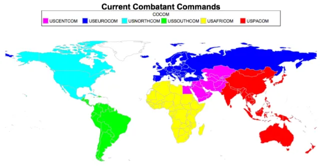
Another way to view the di↵erent regions of the world is from a military perspective through the lens of the United States Combatant Commands. The COCOMs were developed after the United States’ experience in World War II and were established as the military’s way of dividing up the world to more e↵ectively engage in di↵erent a↵airs and conflicts around the world [4]. The COCOMs have a long standing history of their geographic nature in terms of how they are structured and which countries fall under each COCOMs responsibilities. Since their development after World War II, they have largely remained unchanged in structure. Figure 1 shows the current structure of the COCOMs. It is apparent from the map that the current COCOM structure is heavily based on geography.

Military leaders now question the current structure of the COCOMs and considered if there is a more e↵ective alignment of the COCOMs. General Dunford commented in his Senate confirmation hearing on the need to reevaluate the Combatant Commands and consider if there is a more e↵ective way to structure them [5]. The questioning of the current COCOM structure ultimately leads to the question, how should the COCOMs be structured?

(28)

to-Figure 1: Current Combatant Command Structure

gether based on similarities beyond location and economic status. Their study pre-dicted clusters of countries based on psychological, sociological, demographic, and economic characteristics (a priori) and used discriminant analysis to confirm clusters in a split half sample [17]. Their results provide strong evidence to support existence of 10 cultural clusters and provides the possibility for new definitions of regions within the world based on factors outside of geography.

2.5 Overview of Methods

This final section reviews the theory of logistic regression. The most recent and most successful prediction models have used forms of logistic regression as a way to calculate the probability of a nation to transition into or out of conflict. The goal in developing a logistic regression model is the same as in developing a linear model; find the best fitting and most parsimonious model to describe the true relationship between the independent variables, also known as covariates, and the dependent variable [18, p. 1]. While the goals are the same, logistic regression does di↵er in several ways

(29)

from linear regression. Logistic regression is used in situations in which the response variable y is dichotomous, such as in the instance of conflict transitions where either a transition was observed or not in a given year [18]. The parameters in the logistic regression model are estimated through maximum likelihood estimation. Estimations of parameters made through the maximum likelihood estimation technique produces estimated parameters that maximize the probability of obtaining the observed set of data [18, p. 8]. Because of the dichotomous dependent variable, the conditional mean is greater than or equal 0 and less than or equal to 1. The conditional mean is defined in Equation 1.

⇡(x) = E(Y|x) = e

o+ 1+...+ p e1+ o+ 1+...+ p

⇡(x) = estimated probability of success (Y = 1) for given x

(1)

Given the nonlinear nature of the equation, a logit transformation is performed on ⇡(x) to obtain more desirable properties that are seen in linear regression. The logit transformation is defined in Equation 2.

g(x) = ln 

⇡(x)

1 ⇡(x) (2)

The resulting equation after applying the logit transformation, g(x), results in continuous linear parameters, over the range [ ₁,₁]. The antilog of the parameters are interpreted as the estimated increase in the probability of success.

The methods to determine the overall significance of logistic regression models and the significance of parameters is another di↵erence between linear regression and logistic regression. In logistic regression, the overall significance of a model is determined by the Likelihood Ratio Test (LRT) which compares the observed values of the response to the predicted values obtained from the model. The overall significance of the model is obtained by comparing the likelihood of the fitted model with only

(30)

the intercept and the likelihood of the saturated model. This comparison is otherwise known as the G statistic and is represented by the Equation 3.

G= 2ln 

likelihood of fitted model

likelihood of saturated model (3)

The G statistic follows a chi-square distribution with p degrees of freedom where p is the number of independent variable parameters in the model [18]. The null hypothesis for the LRT is that the p coefficients for the covariates in the model are equal to 0 and the null is rejected if theGstatistic is less than the chi-square statistic with p degrees of freedom [18].

The LRT can also be used to determine the significance of parameters in the model. The LRT in this case compares the model without the variable and the model with the variable, assuming all other variables stay in the model. The G statistic in the single variable significance test follows a chi-square distribution with 1 degree of freedom.

One other way that the significance of variables in the model can be determined is by the Wald Test. The Wald Statistic for testing the significance of a single variable compares the estimated parameter to the estimated standard error of the parameter. The equation for a Wald statistic for a single variablei can be represented as seen in Equation 4. Wi = ˆ_i ˆ SE( ˆi) (4) The Wald Statistic, under the null hypothesis that an individual coefficient is zero, follows a standard normal distribution [18]. The LRT and Wald Statistics can be used in combination to determine the significance of the overall model, compare models with or without a certain subset of variables, and determine the significance of individual parameters.

(31)

2.6 Summary

This literature review provides background on previous models and techniques used to forecast conflict transitions of nations, how border conflicts a↵ect a nation’s like-lihood of entering into a state of conflict, and the regional considerations of conflict. Logistic regression and simulation are e↵ective ways to predict and model conflict trends over time and region specific models have produced the most accurate con-flict predictions. Prediction models have been studied mainly based on geographic similarities between nations, but other methods have been proposed to group nations together outside of geographic factors. Furthermore, many of the variables used to predict the onset of conflict overlap throughout the studies. One variable that is mod-eled di↵erently throughout the studies is the influence of border conflict. Geographic proximity measures and demographic variables such as number of refugees have also been used to determine the influence of a neighboring country on another country, but there is no one measure that has consistently been used to model the influence of border conflicts in conflict prediction models.

(32)

III. Methodology

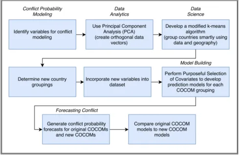
3.1 Overview

This research explores the techniques used to potentially group countries into new COCOM groupings and develop models to forecast nation-state conflict. Section 3.2 describes the methodology used to develop the dataset used in this research in regards to data sources, variable selection, development of the dependent variable, and imputation procedures. Section 3.3 discusses the development of new COCOMs from each country’s current COCOM assignment. Section 3.4 covers the development of the conditional regional models to include discussions on logistic regression and the purposeful selection of covariates. Finally, Section 3.5 examines the model adequacy performance measures used in this research to validate and compare models.

(33)

3.2 Dataset

3.2.1 Database Development

The data for this research is similar to and built o↵ of the data used in the Shall-cross [2] and Leiby [3] studies. This study considers the same 182 countries from the Shallcross [2] and Leiby [3] studies from 2004-2015 and includes 29 of the 30 indepen-dent variables studied in Shallcross [2]. The 182 countries consist of 181 of the 193 United Nations members as well as Palestine which is referred to as West Bank. The variable that was was included in the Shallcross [2] study but not in this study was the Military Expenditure as a percent of government spending. This variable was not included in this study because it was missing almost 50% of the data. The other di↵erences between the data used for this research and the Shallcross [2] study data is the addition of 2015 data for all variables, 2 additional technology related variables, 2 border conflict variables inspired by the variables developed in Leiby’s [3] work, and a minor change in the definition of the dependent variable. These di↵erences are discussed in greater detail in the following sections.

3.2.2 Dependent Variable

The dependent variable, Conflict Transition, is modeled as a binary variable indi-cating a change in conflict status for a country from the previous year. The conflict status of each country in a given year is determined by mapping the country’s highest level of conflict intensity, also known as its HIIK value, in a given year. A HIIK level of 0, 1, or 2 is mapped to the conflict status of 0 indicating that a country is not in a state of conflict. HIIK levels of 3, 4, and 5 are mapped to a conflict status of 1 indicating that a country is in a state of conflict in that given year. The dependent variable Conflict Transition is equal to 0 if there is no change between the conflict

(34)

status of the current yeari and the conflict status of the previous yeari 1. Conflict Transition is equal to 1 if the conflict status in a given year i is not equal to the conflict status in the previous year i 1. Table 1 shows the combinations of values for conflict status in year i 1 and yeariand the respective values for the dependent variable Conflict Transition in year i.

Table 1: Mapping of the Dependent Variable

Conflict Status Yr i 1 Conflict Status Yr i Conflict Transition Yr i

0=Not In Conflict 0=Not In Conflict 0=No Transition

1=In Conflict 1=In Conflict 0= No Transition

0=Not In Conflict 1=In Conflict 1= Transition

1=In Conflict 0= Not In Conflict 1= Transition

3.2.3 Independent Variables

This research uses many variables included in previous conflict prediction studies, but also incorporates several new variables. The variables unique to this study and discussions on specific variable development are discussed in this section. The sources and units of measurement for all independent variables are found in Appendix A.

Internet Users

The Internet Users variable is from the World DataBank World Development In-dicators and describes the number of Internet users per 100 people in a country in a given year.

Mobile Cell Subscriptions

The Mobile Cell Subscription variable is from the World DataBank World Devel-opment Indicators and gives the total number of mobile cellular phone subscriptions in a country in a given year.

Democratic Government Type (Binary Indicator)

Based on previous research, a country having a democratic government or not has been a significant variable in previous conflict modeling e↵orts. While the

(35)

govern-ment type variable does account for a democratic governgovern-ment type, the Democratic Government Type (Binary Indicator) variable served as a more general variable to dif-ferentiate between democratic governments and non-democratic governments. This variable was created by mapping the government type variable. The Democratic Government variable is equal 1 to if government type is democratic. Otherwise, the variable is equal to 0.

Transformed Polity

Both Shallcross [2] and Leiby [3] used the Polity IV variable which originates from the Center for Systemic Peace. The original Polity variable scored the government level based on a -10 to 10 scale with a -10 indicating fully autocratic and a 10 fully democratic [19]. Additionally, the variable indicates if a country experienced a for-eign interruption, anarchy, or was in a transitional state with values of -66, -77, and -88 respectively. The Polity Score spectrum can be divided into three regime cate-gories: autocracies (-10 to -6), anocracies (-5 to +5 and values -66, -77, and -88), and democracies (+6 to +10) [19]. The governments encompassed by the extreme nega-tive values were similar to the types of governments with a value of zero and included in the same regime category. Because these extreme negative values are associated with similar types of governments as those governments included in the middle of the Polity score spectrum, the original polity variable was transformed so that those instances of extreme negative values, -66, -77, and -88, were mapped to zero. This ensured that all instances were in the -10 to 10 scale and could help better identify those countries experiencing more unstable or transitional governments.

Government Type

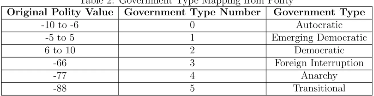
The Government Type variable was used in both Shallcross [2] and Leiby [3] studies as a dynamic variable to indicate a country’s government type. It is a categorical variable which stems from mapping the original Polity Variable into 6 categories as

(36)

shown in Table 2.

Table 2: Government Type Mapping from Polity

Original Polity Value Government Type Number Government Type

-10 to -6 0 Autocratic -5 to 5 1 Emerging Democratic 6 to 10 2 Democratic -66 3 Foreign Interruption -77 4 Anarchy -88 5 Transitional

Percent Border Conflict

The Percent Border Conflict variable is consistent with the border conflict variable in Shallcross [2] and Boekestein [15]. The Percent Border variable is calculated by summing the percent of the perimeter of the border shared with a neighboring country multiplied by the HIIK level of conflict intensity for that country for all countries that share a physical border with a given country. Islands were assumed to not have any neighboring countries. Equation 5 defines the Percent Border Conflict variable.

P ctBCij = n

X

k=1

Hkjpk where

n= number of bordering countries for country i

Hkj = HIIK conflict intensity level for country k in yearj

pk = percent of border country ishares with country k

i= Country ₂_{1,2, ...,182_} j = Year ₂_{2004, ...,2015_}

k= Bordering country

(5)

Average Border Conflict

The Average Border Conflict variable measures the average level of conflict sur-rounding a given nation in a given year. Islands are assumed to not have any

(37)

neigh-boring countries. Average Border Conflict score for a country is defined in Equation 6. AvgBCij = Pn k=1Hkj n where

n= number of bordering countries for country i

i= Country 2{1,2, ...,182} j = Year ₂_{2004, ...,2015_}

(6)

Binary Border Conflict

The Binary Border Conflict variable is consistent with the binary border conflict variable in the Leiby [3] study and indicates if at least one bordering country is in a state of conflict in a given year. Islands are assumed to not have any neighboring countries. Binary Border Conflict score for a country is defined in Equation 7.

BinBCij = 8 > > < > > :

1 if Hkj 3 for any country bordering country i

0 if otherwise

i= Country 2{1,2, ...,182} j = Year ₂_{2004, ...,2015_}

(7)

3.2.4 Challenges working with the Data

One of the challenges in working with a large open source data set was determining which variables to include in the study and how to handle the missing values in the

(38)

dataset. The base set of variables are those 30 variables identified in the Shallcross [2] study. The amount of missing data in each of those variables led to removing the Military Expenditure as a percent of government spending; almost 50% of its values were missing. To compare di↵erent border variables in our study two additional border conflict variables similar to the ones used in the Leiby [3] study in addition to the variables from the Shallcross [2] study were added. The Mobile Cell Subscription and Internet users variables helped investigate the e↵ect technology access has on conflict.

After determining which variables to include in the study, missing data gaps in the full dataset needed consideration. There are a number of ways in which missing data can be handled with varying levels of complexity, validity, and the nature of randomness of the missing data. This study assumed all data are missing at random meaning that the probability of a observation having a missing value for a variable may depend on the known values, but not on the value of the missing data itself [20]. One of the simplest ways to handle missing data is to only consider complete cases which have no missing values within all the fields for an observation. Only considering those complete cases that had no missing values means losing over 50% of the observations in the dataset. Therefore, imputation methods were used to fill in the missing data with appropriate values that would allow for analysis with as much information as possible, but maintain the integrity of the original data.

Before using general imputation methods on the whole dataset, a preliminary analysis of the missing values in the dataset looked for any patterns within the missing data and considered using prior knowledge of the data to fill in missing values. There were many values missing for South Sudan from 2004-2010. South Sudan gained independence from Sudan in 2011 [21]. Using this knowledge, South Sudan’s missing values for 2004-2010 were imputed with the available and corresponding Sudan values.

(39)

Arable land was another variable that had a pattern of missing data. The majority of missing values for the arable land variable were 2015 values. Because the amount of arable land does not change very quickly in the span of a year or two, the missing values were imputed by carrying forward the last original value of arable land data for a given country.

The population variable only had missing values for Eritrea from 2012-2015. The missing values were imputed using a time series forecast of the population based on the population in Eritrea in 2011 and assuming a 2% growth rate. The 2% growth rate is consistent with the average growth rate of Eritrea’s population from 2004-2011. The last variable using a specific imputation method based on prior knowledge was the Polity variable. There are 3 variables included in the dataset that provide information on the governing structure within a country: regime type, polity, and government type. Regime type was first cited in the CIA study by Goldstone as a significant predictor of political instability [7]. Boekestein [15] used a simplified, mapped version of the original regime type variable which originally had 57 govern-ment descriptions. The simplified 3 level indicator variable developed in Boekestein [15] was also used in Shallcross [2] and Leiby [3] and is static for every year for every country in the study. There were no missing values for this variable. The original Polity variable indicated the government level based on a -10 to 10 scale with a -10 indicating fully autocratic and a 10 fully democratic and had indicators for countries with anarchies, transitioning governments, or governments experiencing a foreign in-terruption. Polity did contain some missing values which were necessary to fill in before creating government type which is a categorical variable that maps the Polity values. The missing values for Polity were imputed based on the countries regime type using the following mapping scheme from regime type’s three levels as seen in Table 3.

(40)

Table 3: Mapping of Regime Type to Fill in Missing Polity Values

Regime Type Corresponding Imputed Polity Value

Central Ruling Party -10

Emerging, Transitional, Recent Change, Disputed 0

Democratic 10

After applying the specific imputation methods to the variables previously men-tioned, there were two main methods used to impute the remaining missing data values: multivariate normal imputation and univariate imputation. These two meth-ods were employed using JMP Missing Values Utility software. The multivariate normal imputation method fills in missing values based on the multivariate normal distribution and uses least squares imputation [22]. This method only works with continuous data and is the preferred method of imputation compared to univariate imputation because it provides an estimate of the value based on the information in other rows and columns of the data rather than only considering one variable. A problem encountered when using this method was getting estimates for missing data that were not within the bounds of the original variable. For each variable requir-ing imputation, multivariate imputation was used first. If the imputed data did not resemble the original data, the univariate imputation method was used instead.

The univariate imputation method only considers a single column of data to impute and fills in the missing data points for that column with the mean of the original values for the variable. A summary of the imputation methods used for each variable is found in Appendix A.

After imputing all missing values with the specified imputation techniques the Kolmogorov-Smirnov (KS) Test tests how similar the imputed data is to the original data. The KS test is a goodness of fit test used to compare the distributions of a sample to some specific distribution or another sample [23]. This test was conducted in R to compare the distributions of the original data to the imputed data for each

(41)

continuous variable. The test statistic for the KS Test is based on the maximum di↵erence between the cumulative distribution function (CDF) of each sample. Under the null hypothesis, the distributions are the same. An alpha of 0.05 was used as the significance level for this test. All but two variables, Refugee Asylum and Caloric Intake, passed the KS Test meaning that there is no statistical di↵erence between the distributions of the of the non-imputed data and the imputed data.

3.3 Country Grouping Development

This section details how new Combatant Command groupings were developed us-ing principal component analysis and the Modified K-means Algorithm. The current COCOMs and the new COCOM groupings developed from the methodology discussed in this section were the groups used to build conflict prediction models in the model building portion of the study.

3.3.1 Data for New COCOM Development

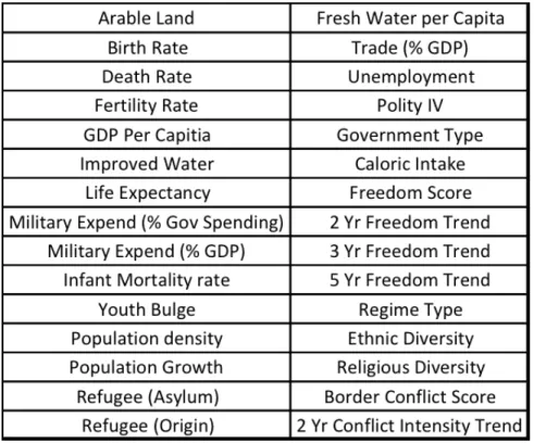
The data used for developing new COCOM groupings was based o↵ of the data used in the Shallcross study [2]. The data consisted of 30 data elements which describe various political, military, economic, social, information and infrastructure character-istics of 182 countries from the years 2004-2014. For this portion of the analysis only one year of data for each of the 182 countries was used. The year 2014 was chosen as the dataset to analyze because it was the most recent year that had the most com-plete data. Additionally, regime type and government type were the only categorical variables in the dataset and were transformed into binary indicator variables for each level of the respective variable. Thus, the final set of variables used for principal com-ponent analysis consisted of 35 numeric variables for the year 2014 for 182 countries. The list of variables for this portion of the analysis can be found in Figure 3.

(42)

Figure 3: Variables used in PCA and Country Grouping

3.3.2 Principal Component Analysis

Principal component analysis (PCA) is a data reduction technique used to reduce the dimensionality of a larger dataset and investigate underlying relationships of the original variables. PCA uses orthogonal linear combinations of the original variables, also known as principal components, to produce a lower dimensionality set of vari-ables that describe commonalities within the data and account for as much of the variation in the original data as possible [24, p. 20]. The principal components (PC) are extracted from the data such that the first principal component accounts for the largest amount of the total variation in the data and each subsequent principal com-ponent accounts for less variation than the previous. The equation for themth _{PC is} found in Equation 8 [24, p. 25].

(43)

P C(m) =w(m)1X1+w(m)2X2+...+w(m)1Xp

Xj = Observed variable j, j = 1,2, ..., p

(8)

The weights w are chosen to maximize the ratio of variance of P C(m) to the total variation such that the sum of the squared weights is equal to 1 and the principal components are orthogonal [24, p. 24]. The principal components are based on the eigenvalues and eigenvectors of the correlation matrixR of the full standardized data matrix. PCA can be performed on unscaled, unstandardized data, but may give misleading results as to which variables have the most impact on the variation in the data. Because the variables in the dataset have di↵erent scales, the data was standardized at the beginning of the PCA to ensure that all the data was measured on the same scale and could be compared on a common scale. The standard procedure for calculating PCs is as follows:

1. Calculate the correlation matrix R of the data matrix X where X is an n x p matrix where n= number of observations and p= number of variables.

2. Calculate the eigenvalues and eigenvectors from R.

3. Use eigenvectors to calculate the Loadings Matrix, L, and determine number of components to retain.

4. Calculate scores for each observation for each component using Loadings matrix. The maximum number of components calculated from the data is equal to the number of original variables in data. Since the goal of PCA is to reduce the number of variables needed to explain the variance in the data, a subset of principal components are used while still maximizing the variance in the original data. A dimensionality assessment is conducted to reduce the number of components used in the analysis while still retaining as much original variation as possible in the data. Horn’s Test is

(44)

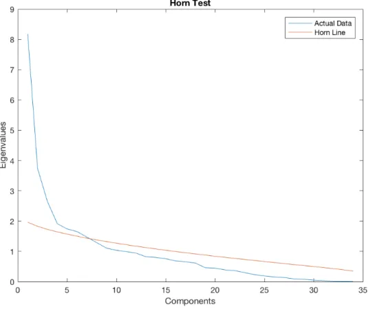
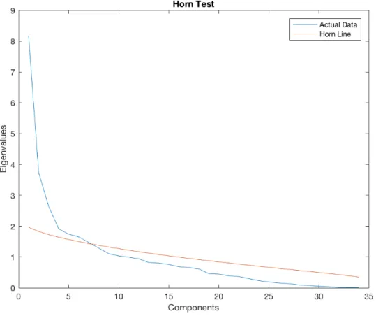
one such dimensionality assessment where the calculated eigenvalues from the data are plotted in descending order of magnitude along with a theoretical line based on normally and independently distributed random variates from a population whose correlation structure is characterized by an identity matrix [24, p. 49]. A Horn’s Curve plot consists of plotting the theoretical and actual eigenvalues versus the number of components. In Horn’s Test, the criterion for the number of principal components to retain is the number of components at the point where the theoretical and actual lines intersect. An example of a Horn’s Curve plot is shown in Figure 4.

Figure 4: Example Horn’s Curve Plot

The red line in the plot represents the theoretical data and the blue line represents the actual observed data. The point at which they cross is around 7 components. Because the actual data line remains close to the theoretical line until about 9

(45)

com-ponents, additional components can arguably be retained. Nine principal components are retained.

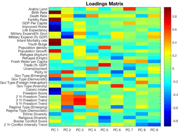
Next, the Loadings matrix is calculated. The Loadings matrix describes the cor-relation between the variables and each component [24]. The Loadings matrix is calculated through the following equations shown in Equation 9.

L=D 1/2AR⇤1R/2

D= Diagonal matrix of R

AR = Eigenvectors of R

⇤R= Eigenvalues of R

(9)

The Loadings matrix explains the correlation between the variables within each component and gives a sense as to which variables have the greatest influence on each component [24]. This technique can be informative in explaining what is common among groups of observations and explaining the variance within large datasets. By highlighting the variables that have the highest correlation in each of the compo-nents, insight can be gained as to what aspect of the data each principal component describes.

The final portion of PCA consists of calculating and plotting the principal compo-nent scores for each observation. A score is calculated for each observation for each of the retained principal components. These scores are obtained by multiplying the linear combination of the original variables to the appropriate data for each observa-tion. The score matrix S contains the score for each observation for each principal component. The calculation of the score matrix S is shown in Equation 10.

(46)

S =XsD 1/2AR

Xs= Standardized data matrix

D= Diagonal matrix of R

AR = Eigenvectors of R

(10)

The component scores encompass most of the information from the original dataset and can be used to compare how similar observations are based on the data. Plotting the scores in di↵erent pairings allows a visual comparison of observations. A score plot is produced by plotting two component scores for each observation as the x and y coordinates in a 2-dimensional plot.

Even though this technique is not explicitly a classification technique, sometimes patterns exist within the data which can be visualized in the plots of principal com-ponent scores. Plots of combinations of two principal comcom-ponents scores for each observation are created to analyze similarities between countries under the current Combatant Command structure. The color and shape of the data points represent the group a country is a part of, in this case COCOM. Visually inspecting the score plot, provides an indication of any patterns or similarities between countries based on data. The results from the principal component analysis were used in the implementation of the Modified K-means Algorithm.

3.3.3 Modified K-means Algorithm

Conducting principal component analysis reduces a highly-dimensional data set into a smaller and easier to visualize dataset and compares observations on a common scale. The score plots present clusters of similar observations based on the groupings and the ability to perform cluster analysis on the data. There are several di↵erent ways to conduct cluster analysis depending on what assumptions are made about the

(47)

data and the desired outcome from the analysis. K-means clustering was the chosen method for cluster analysis and inspired the development of a Modified K-means Algorithm.

K-means clustering partitions observations within a data set into K distinct and mutually exclusive clusters [25, p. 387]. The objective of K-means clustering is to partition the data to minimize the within cluster variation [25, p. 387]. In K-means clustering the number of clusters, K, is assumed known and predefined at the begin-ning of the cluster analysis.

There are several ways to define and compare variation between observations. The most common way suggested in An Introduction to Statistical Learning is using the squared Euclidean distance between observations [25]. The scores from principal component analysis give a means to compare the observations based on data char-acteristics on a common scale. The di↵erence between component scores between two observations can be compared to determine how similar the observations are to one another. The distance between the scores can be thought of as a measure of how similar the two observations are and a distance can be calculated between the two points. The squared Euclidean distance between observations was chosen as as the way to calculate the distance between two points with x and y coordinates (one principal component score for the x and one for the y) for each observation. The Euclidean distance between observations on a score plot was the comparison metric chosen to determine how similar observations were to each other. The objective func-tion for solving the K-means clustering problem using the Euclidean distance between observations as the comparison metric is shown in Equation 11.

min C1...Ck ( _K X k=1 1 |Ck| X i,i0₂_C_k p X j=1 (xij xi0j)2 ) (11) In Equation 11, |Ck| is the number of observations in the kth cluster and the

(48)

Euclidean distance between an observationi and every other observationi0 _{that is in}

the cluster is calculated by (xij xi0_j)2 [25].

The large number of possible ways to partition n observations into K clusters makes this a very large and difficult problem to solve. An Introduction to Statistical Learning proposes a simple and elegant approach to solve this problem for a local optimum with the K-means algorithm [25, p. 388]. A summary of the K-means clustering algorithm proposed in the text can be seen in Algorithm 1.

Algorithm 1Pseudocode for the K-means Clustering Algorithm

Determinek number of clusters in data

Assign each observation a number 1 tok to serve as initial cluster assignment for each observation

while cluster assignments change do

a: Calculate the centroid of each cluster 1 tok . The centroid of thekth cluster is defined as the vector of means for each feature for observations in thekth cluster b: Assign each observation to the closest centroid as determined using the Eu-clidean distance between each observation and each cluster centroid.

This algorithm is based on the assumption that there exist K mutually exclusive clusters in the data, with unknown cluster membership. Another assumption is that the closer the distance between two observations, the more similar the two observa-tions are to one another. A third assumption is that all observaobserva-tions are assigned to a cluster. One limitation in this algorithm is that the algorithm finds a local optimum, not a global optimum, and the results from the algorithm depend on the initial setting of the clusters.

The K-means algorithm provides a way to group observations based on data simi-larities. In this study the observations are individual countries and the data represent various political, military, economic, social, infrastructure, and information

(49)

character-istics of a country. The analysis needs to compare countries based on data similarity and location. To develop new COCOM groupings of countries location is used in a clustering algorithm to ensure that the new COCOMs would be mostly geographi-cally clustered and somewhat similar to the current structure. A modified k-means clustering algorithm, called the Modified K-means Algorithm, incorporates both data characteristics and geographic proximity in grouping similar countries together. Com-paring countries’ similarities involved PC scores 1 and 2 for each country. ComCom-paring the geographic proximity of each country to one another used the Latitude and Lon-gitudinal coordinates for each country’s capital city. The geographic similarity metric was calculated using the Great Circle distance between countries’ capital cities. This distance was normalized and scaled to coincide with the scale of the principal compo-nent scores to combine the data and geographic similarity metrics into a single, total distance or similarity metric. The pseudo-code for the Modified K-means Algorithm, which clusters similar countries together based on data similarity and geography, is described in Algorithm 2.

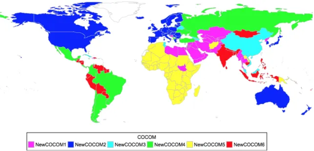
Applying the Modified K-means Algorithm to the 2014 data for the selected 182 countries resulted in groups of countries that were similar based on data and geog-raphy. The groupings for the conflict probability models were developed from the current COCOM structure and the results obtained from the Modified K-means Al-gorithm.

3.4 Model Building Procedure

The goal of many model building procedures is to build the most parsimonious model that accurately reflects the true outcome experience of the data [18]. This study uses the purposeful selection of covariates (PSC) model building method as proposed by Hosmer, Lemeshow, and Sturdivant in Applied Logistic Regression [18].