PREDICTION OF LEAF SPRING
PARAMETERS USING ARTIFICIAL
NEURAL NETWORKS
Dr.D.V.V.KRISHNA PRASAD, J.P.KARTHIK
Department of Mechanical Engineering, RVR&JC Engineering College,
Guntur (Dist)-522019(A.P)
[email protected],[email protected]
Abstract:
In this paper an attempt is made to predict the optimum design parameters using artificial neural networks. For this static and dynamic analysis on various leaf spring configuration is carried out by ANSYS and is used as training data for neural network. Training data includes cross section of the leaf, load on the leaf spring, stresses, displacement and natural frequencies. By creating a network using thickness and width of the leaf, load on the leaf spring as input parameters and stresses, displacement, natural frequencies as target data, stresses, displacement and natural frequencies can be predicted. By creating a network using values of stresses, displacement and load as input parameters to the network, thickness and width of the leaf as Target values, thickness and width of the leaf spring can be predicted. For independent values the two networks are tested and results are compared with the results obtained from ANSYS. Using PRO/E leaf spring was modeled and in ANSYS it was analyzed.
Keywords: Leaf Spring, ANSYS, Artificial Neural Networks. 1. Introduction
In a leaf spring design procedure in order to optimize the design parameters, every time tests are to be done on leaf spring to obtain displacement and stresses using ANSYS. Again dimensions are to be changed keeping this displacement, stresses within the limits. An alternate method is introduced to predict optimal design parameters using artificial neural networks. For this technique, ANSYS package is used for obtaining displacement, stresses and natural frequencies for number of configurations of leaf springs by varying the cross section of leaf that is width and thickness of the leaf, and load on the leaf spring. A network is created using results obtained from ANSYS. This network is used for predicting stresses and displacement. For independent values of width, thickness of the leaf and load, displacement and stresses are found from the network. Analysis for these values is carried out. The results obtained from network and ANSYS are in close agreement. For this analysis the leaf spring considered is having following specification
Number of leaves: 1 leaf s to 22 leafs Leaf span: 200mm to2400mm Camber 250mm max
ID of the eye: 12mm to 65mm Leaf width: 40mm to 120mm Load 20,000Kg max
Material selected is manganese silicon steel (steel 55Si2Mn90) and the properties are Young modulus, E=2.1E5 N/mm2
Density=7.86EKg/mm3 Poisons ratio=0.3
Tensile stress=1963 N/mm2 Yield stress =1470 N/mm2
From these specifications following four configurations of the leaf spring are taken as constant, their values are Number of leafs = 5
2. Modeling &Analysis of steel leaf spring
In this project each leaf of leaf spring is designed using modeling software PRO/E 4.0. PRO/E Version 4.0 is the first release of the next generation of PTC(Parametric Technology Corporation)., and addresses advanced mechanical process centric design requirements. In addition to leading edge feature - based design functions, it includes highly productive capabilities for the design of mechanical assemblies and for drawing generation. Modeling is done by using PRO/E 4.0 (Version).
For the part models first we select the part design and we draw the profile of the model.
After drawing the part profile then continue with sketch and extrude it to measured length.
We have to constrain all parameters of the dimensional that we have taken from the physical model.
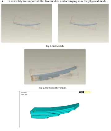
After modeling the five leaves we can create the assembly of the models.
In assembly we import all the five models and arranging it as the physical model.
Fig 1.Part Models
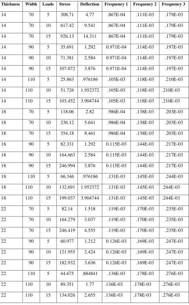
Fig 2.pro/e assembly model
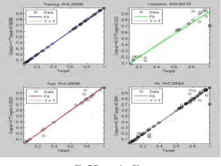
Fig 3.It shows the leaf spring which is imported to ANSYS
The above shows the leaf spring which is imported from PRO/E to ANSYS. The following are the steps involved in the Analysis of leaf spring.
The ANSYS setup utility automatically creates a program group and places a shortcut icon on the desktop. By double clicking on the icon, the default ANSYS desktop
Import Assembly part of leaf spring which is in IGES format by selecting file > import > IGES from the menu bar.
Select structural from preferences. Click on preferences > structural > Ok.
Enter properties of material in the dialog box which is shown below. It appears by selecting Preprocessor > Material properties > Structural > Linear > Elastic > Isotropic.
Mesh the part using Mesh Tool in Preprocessor.
The part with meshing is obtained below
Fig.4 Mesh Part
3. Boundary conditions
Leaf spring is mounted on the axle of the automobile; the frame of the vehicle is connected to the ends of leaf spring. The ends of the leaf springs are formed in the shape of eye. The front end of the leaf spring is coupled directly with the pin to the frame so that the eye rotates freely about the pin but no translation is occurred. The rear eye is connected to the shackle which is flexible link; the other end of shackle is connected to the frame of the vehicle. The rear of the leaf spring has the flexibility to slide along the X-direction when the load applied on the spring and also rotates about the pin. The link associates during load applied and removed.
So, for analysis because of symmetry, leaf spring is considered as the cantilever beam which is fixed at one end and load is applied at other end. All DOF are restricted on one side and on other side load is exactly applied at the center of leaf spring width.
The static analysis is carried for the configurations shown in table and the results are tabulated in table considering
Length of the first leaf =1000mm Length of the second leaf =1000mm Length of the third leaf =850mm Length of the fourth leaf =600mm Length of the fifth leaf = 350mm
Fig.5 Constrained Part Fig.6 Loaded Part
4. Steps involved for Modal Analysis Using ANSYS
Preferences > structural
Preprocessor
Element Type> 8 Node Solid 45
Material Properties> Material Models> Structural > Elastic >Isotropic> Ex=2.1e5; Px=0.3 Meshing> Mesh Tool > Smart Size = 3> Free Mesh
Solution
Analysis Type> New Analysis> Modal
Analysis Options > Block LonczMethod ; Modes to be expand =3; Modes to be extract =3 Solve > Current L.S
General post processor Read Results > First Set
Read Results > Second Set
Plot Cntrls> Deformed Results > Deformed +Undeformed Shape Read Results > Last Set
Plot Cntrls> Deformed Results > Deformed +Undeformed Shape
Table 1.The results for various configurations shown in table are tabulated in table
Thickness Width Loads Stress Deflection Frequency 1 Frequency 2 Frequency 3
14 70 5 308.71 4.77 .867E-04 .111E-03 .179E-03
14 70 10 617.42 9.541 .867E-04 .111E-03 .179E-03
14 70 15 926.13 14.311 .867E-04 .111E-03 .179E-03
14 90 5 35.691 1.292 0.971E-04 .114E-03 .197E-03
14 90 10 71.381 2.584 0.971E-04 .114E-03 .197E-03
14 90 15 107.072 3.876 0.971E-04 .114E-03 .197E-03
14 110 5 25.863 .976186 .105E-03 .118E-03 .210E-03
14 110 10 51.726 1.952372 .105E-03 .118E-03 .210E-03
14 110 15 103.452 3.904744 .105E-03 .118E-03 .210E-03
18 70 5 118.06 2.82 .986E-04 .138E-03 .203E-03
18 70 10 236.12 5.641 .986E-04 .138E-03 .203E-03
18 70 15 354.18 8.461 .986E-04 .138E-03 .203E-03
18 90 5 82.331 1.292 0.115E-03 .144E-03 .217E-03
18 90 10 164.663 2.584 0.115E-03 .144E-03 .217E-03
18 90 15 246.994 3.876 0.115E-03 .144E-03 .217E-03
18 110 5 66.346 .976186 .131E-03 .145E-03 .244E-03
18 110 10 132.691 1.952372 .131E-03 .145E-03 .244E-03
18 110 15 199.037 3.904744 .131E-03 .145E-03 .244E-03
22 70 5 82.14 1.518 .119E-03 .170E-03 .235E-03
22 70 10 164.279 3.037 .119E-03 .170E-03 .235E-03
22 70 15 246.419 4.555 .119E-03 .170E-03 .235E-03
22 90 5 60.977 1.212 0.126E-03 .169E-03 .247E-03
22 90 10 121.955 2.424 0.126E-03 .169E-03 .247E-03
22 90 15 182.932 3.636 0.126E-03 .169E-03 .247E-03
22 110 5 44.675 .884841 .136E-03 .178E-03 .276E-03
22 110 10 89.351 1.77 .136E-03 .178E-03 .276E-03
5.Artificial Neural Network
The term Artificial Neural Network (ANN) comes from the intended analogy with the functioning of the human brain adopting simplified models of “biological network”. In an ANN, the neurons or the processing units may have several input paths corresponding to the dendrites. The units combine usually by a simple summation, that is, the weighted values of these paths. The weighted value is passed to the neuron, where it is modified by threshold function such as sigmoid function. The modified value is directly presented to the next neuron. A feed forward Artificial Neural network consist of layer of processing units, each layer feeding inputs to the next layer in a feed forward manner through a set of connection weights. Once the network weights and biases have been initialized the network is ready for training. The training process requires a set of examples of proper network behavior – network inputs P and network target outputs T .The neural network training is accomplished by presenting a sequence of training vectors, each with associated target output vector. The weights are then adjusted according to the learning algorithm. The network is initiated with one input layer, one hidden layer and one output layer. The number of neurons in each layer is given respectively. In general the outputs will not be same as the target or desired value.
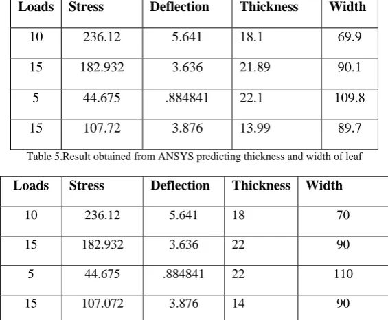
The data in the table 1 is used to train the network. For creating networks load on the leaf spring, width of the leaf and thickness of the leaf were taken as input values and maximum displacement, stress, frequencies are taken as target values. The target values are normalized between 0 and 1. The network type is feed-forward back propagation, number of neurons are 20, transfer function is TRANSIG, training function is TRAINLM, adaption learning function is LEARNDGM, performance function is Mean Square Error, and number of layers are two. The network is trained and tested many times for its accuracy to get the best network. The regression plot for the network is shown in figure 7.
Fig.7 Regression Plot
6. Results
The network is simulated for independent values of load on the leaf spring, width of the leaf and thickness of the leaf the results obtained from artificial neural network and ANSYS are tabulated in table 2 & table 3.
Table 2.The results obtained from Artificial Neural Network
Thickness Width Loa ds
Stress Deflecti on
Frequency 1 10--3 Frequency2 10--3 Frequency 3 10--3
20 80 10 187.99 2.3132 .1175 .2145 .23064
19 100 13 150.48 2.7546 .124 .23328 .24546
15 90 8 107.06 3.73021 0.0971 .1461 .19518
21 105 14 149.15 2.923 .134 .17524 .25193
Table 3.The results obtained from ANSYS
Thickne ss
Width Loa ds
Stress Deflect ion
Frequency1
10--3 Frequency2 10--3 Frequency 3 10--3
20 80 10 183.34 2.3343 .1083 .21 .246
19 100 13 149.75 2.7956 .154 .233 .279
15 90 8 109.45 3.712 0.1127 .1430 0.19331
Similarly network is created for predicting width and thickness of the leaf. For predicting these values load, stresses and deflection are input values and width of the leaf, thickness of the leaf are target values to the network. For different values of load, stresses and deflection thickness of the leaf and width of the leaf are predicted from the network and results are tabulated in table 4 and results from ANSYS are tabulated in table 5.
Table 4.Result obtained from Artificial Neural Network predicting thickness and width of leaf
Loads Stress Deflection Thickness Width
10 236.12 5.641 18.1 69.9
15 182.932 3.636 21.89 90.1
5 44.675 .884841 22.1 109.8
15 107.72 3.876 13.99 89.7
Table 5.Result obtained from ANSYS predicting thickness and width of leaf
Loads Stress Deflection Thickness Width
10 236.12 5.641 18 70
15 182.932 3.636 22 90
5 44.675 .884841 22 110
15 107.072 3.876 14 90
7. Conclusion
In this study, stresses, deflection and the frequency response of leaf spring under different conditions is predicted using Artificial Neural Network approach. This study indicates that ANN offers an attractive route to predict structural as well as dynamic responses and helps us to reduce the modeling and computational time that goes in computer simulation. It shows that ANN can be used in quick, approximate response predictions.
Acknowledgments
The authors were grateful and an indebted to the Department of Mechanical Engineering of Mechanical engineering, RVR&JC College of Engineering for providing the excellent lab and library facilities .
References
[1] TirupathiR. Chandrapuatla & Ashok D.Belgundu,” Introdution to finite elements Engineering”. Third Edition- Pearson Education pvt.Ltd 2002
[2] S.S Rao, “ The Finite Element Method in Engineering”. Third Edition- Butterworth Heimann Publications-2001
[3] T.V.S Sundarrajamurthy, N Shanmugam “Machine Design”- Eigth Edition-published by M.Sethuraman, Anuradha Agencies-2000. [4] http:// www. Mathworks.com/help/toolbox/nnet/rn/rn.html
[5] http://www.learnartificialneuralnetworks.com/