Abstract: We explored the statistics of filtering of simple patterns on a number of deterministic and

Article

Filtering Statistics on Networks

G. J. Baxter1_{, R. A. da Costa}1_{*, S. N. Dorogovtsev}1_{and J. F. F. Mendes}1

1 _{Department of Physics, University of Aveiro de & I3N,}

Campus Universitário de Santiago, 3810-193 Aveiro, Portugal * Correspondence: [email protected]

Abstract: We explored the statistics of filtering of simple patterns on a number of deterministic and random graphs as a tractable simple example of information processing in complex systems. In this problem, multiple inputs map to the same output, and the statistics of filtering is represented by the distribution of this degeneracy. For a few simple filter patterns on a ring we obtained an exact solution of the problem and described numerically more difficult filter setups. For each of the filter patterns and networks we found a few numbers essentially describing the statistics of filtering and compared them for different networks. Our results for networks with diverse architectures appear to be essentially determined by two factors: whether the graphs structure is deterministic or random, and the vertex degree. We find that filtering in random graphs produces a much richer statistics than in deterministic graphs. This statistical richness is reduced by increasing the graph’s degree.

Keywords: filtering; information; degeneracy; entropy; relevance; resolution; complexity; complex networks

1. Introduction

Filtering is the processing of an input signal to produce an output signal according to some rule, based on the content of the input. The filter does not add information, with the number of possible outputs being less than (or at most equal to) the number of possible inputs. Thus, outputs are degenerate: multiple inputs map to the same output. Even very simple filters can produce a

complex distribution of degeneracies [1]. This characteristic, of a nontrivial mapping of a configuration

space to a smaller set of final configurations, also appears in sampling, compression and more general

information processing [2,3], and in numerous complex systems, including the basins of attraction of

local minima in spin glasses, and deep learning neural networks [4–6]. Understanding the statistics of

degeneracies can give important insight into these systems. In a previous work [1], we showed that a

simple filtering problem produces analogous behaviour of the degeneracy distribution to these more complex systems, and that one can obtain exact results up to large system sizes that are simply not accessible in more complex problems.

Numerous studies have shown that the heterogeneous structure of interactions between elements of a complex system, usually represented as a complex network, can have a profound effect on the

properties of the system [7]. Here we examine a simple filtering process on a network. The input

consists of the binary states of nodes in a given network. The filter outputs a 1 for every instance of a particular pattern of states on a node and its immediate neighbours, and a 0 when the pattern is absent.

This generalises the filtering problem examined in Ref. [1] for binary inputs in a cyclical string (ring).

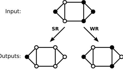
The process applied to a small graph is represented in Figure1. We studied this problem on a variety

of degree-regular graphs. We studied this problem on a variety of degree-regular graphs. We show that one may find the exact degeneracy distribution corresponding to the complete set of all possible inputs, up to relatively large system sizes, for any given graph. Just as in our previous study on rings,

we show that the principal characteristics of the degeneracy distribution are described asymptotically by three key numbers. These numbers may be obtained exactly by simple arguments.

SR WR

Input:

Outputs:

Figure 1.Application of different filters to a set of zeros and ones place on a graph. Each node of the input and output graphs is in one of two states, namely 0 (open circles) or 1 (closed circles). In the SR filter, an output node is one only when the corresponding input node is one and all its neighbours are zero. In the WR filter, an output node is one when the corresponding input node is one and one or more of its neighbours are zero.

This problem serves as a tractable simple model to explore information processing in complex systems. In a graph, the connections between nodes create complex interactions between the

filter output at each node. We show that the degeneracy distribution correctly captures this

complexity. In particular, the entropy of the degeneracy distribution, called therelevance[8] is lower

in deterministically constructed graphs, and higher in random graphs. We show that relevance is maximum when the graph degree takes its smallest value greater than two. We compared two different filters, and found that the stronger filter (detecting less easily satisfied conditions) is more informative,

because it is more sensitive to the state of neighboring nodes. Interestingly, as Figure6demonstrates,

our results for regular graphs of diverse architectures essentially depend only on a vertex degree.

2. Results

2.1. Filtering statistics on a ring

For orientation, we begin by studying nodes located on a ring. The input is a set ofNstrings of

zeroes and ones{xi},xi =0, 1, of lengthn, assuming the periodic conditionx1=xn+1. We consider

the complete set of all possible unique inputs. Its sizeNis determined by the sizenof inputs,N=2n.

The filter works as follows: every instance of a specific pattern in the input (a short sequence of ones and zeroes) is marked by a one in the corresponding position in the output. All other positions are marked with zeroes. Multiple inputs correspond to the same output, creating a distribution of

degeneracies of the outputs. We illustrate the results from a simple example filter pattern in Figure2(a)

and (b). We observe complex degeneracy distributions reminiscent of those observed in, for example,

Ref. [9].

The filter pattern may be arbitrary, but for illustrative purposes we will consider in particular a family of filters consisting of a string of ones with zeroes at either end: 010, 0110, 01110, etc. The

length of the filter,w, can be used as a crude control parameter to observe the effects on resolution and

relevance (see below). For convenience, we use the notation 1lto indicate a chain oflones. Thus the

filter of lengthwis 01w−20. In principle, for each of the 2npossible inputs we can obtain, one by one,

an output numerically. In practice, we use a more efficient algorithm described in Ref. [1]. Other types

101 ₁₀3 ₁₀5 ₁₀7 ₁₀9 d

100

101

102

103

104

105

106

N

(

d

)

(a)

n= 36

101 ₁₀3 ₁₀5 ₁₀7 ₁₀9 d

100

101

102

103

104

105

106

107

Ncum

(

d

)

(b)

101 ₁₀3 ₁₀5 ₁₀7 ₁₀9 d

100

101

102

103

104

105

106

N

(

d

)

(c)

6×6

101 ₁₀3 ₁₀5 ₁₀7 ₁₀9 d

100

101

102

103

104

105

106

Ncum

(

d

)

(d)

Figure 2.Degeneracy distribution (a) and cumulative degeneracy distribution (b) for the filter 010 on a ring, and for its generalization on a torus, which is a 1 with four neighboring 0’s [panels (c) and (d)].

2.1.1. Degeneracy distribution

We obtained the number of outputsN(d)for the full spectrum of degeneraciesdfor a variety

of filters. The degeneraciesdi,i=1, ...,D, form a discrete spectrum of values wheredDis the largest

degeneracy, andd1=1. A few examples of the degeneracy distributions and cumulative degeneracy

distributions are shown in Figure2. HereNcum(di)≡∑Dj=iN(dj). In particular, the total number of

outputs is given byM(n) =Ncum(d1). The cumulative degeneracy distribution is broad, but decays

more rapidly than a power law.

The tail of the cumulative distribution has a notably complex structure resembling a staircase, with steep jumps between steps. The heights of these jumps are especially large in the region of high degeneracies. Similar structures may be observed in real systems, see for example Figure 3 of Ref.

[9]. As shown in Ref. [1], when the number of ones in the output is few, and some or all of them

are separated by large gaps, such outputs have very similar but not exactly equal degeneracies for

finiten. These closely located degeneracies lead to the staircase structure observed in the cumulative

distribution.

Let us consider the evolution of the degeneracy distribution (and cumulative distribution) with

input sizen. The largest degeneracydD(n)corresponds to the output with all zeroes, and for large

n, grows asdD(n)∼=zn_d, where the value ofzddepends on the specific filter. NaturallyN(dD,n) =1.

The number of outputs with degeneracy 1 behaves asN(1,n)∼=zna. Meanwhile the total number of

outputs,M(n)is asymptoticallyM(n)∼=zn_g. Together, these three key constants,zd,zgandza, delimit

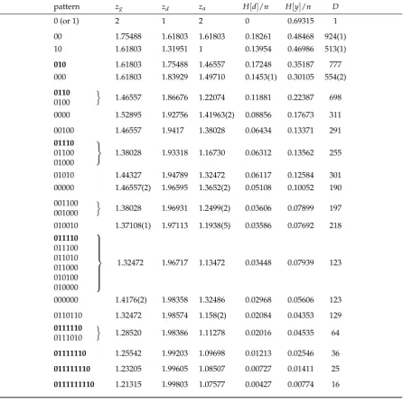
the asymptotic behaviour of the degeneracy distribution [1]. We list these numbers for a selection of

short filter patterns on a ring in Table1.

Rather surprisingly, one may obtain these asymptotic behaviours, and exact expressions for the

constantszg,zdandzathrough simple arguments. Each output consists of isolated ones separated

by strings of zeroes of various lengths. By careful consideration of how valid outputs for a larger

ncan be constructed by adding specific segments to shorter outputs, one may construct recursive

relations for the key quantitiesM(n),dD(n)andN(1,n), whose asymptotics are given byzg,zdandza.

To demonstrate this, we focus on the particular family of filter patterns consisting of a chain of ones with a zero at each end. The shortest such pattern is 010. Each member of this set may be indexed by

the length of the filter,w≥3. The filter pattern lengthwdetermines the minimum number of zeroes,

2.1.2. Effect of filter length

In analogy with complex systems, we can consider each filter pattern as sampling the hidden state

of a complex system [1]. The length of these filters acts as a crude control parameter of our sampling.

Intuitively, we expect shorter filters to be more informative. The resolution of a sampling process, defined as the entropy of a sample:

H[y] =−_N1

N

∑

i=1

log

di N

=−

∑

d

dN(d,n)

N log

d N

(1)

is a measure of the ability to distinguish, at the output, between different input states [8]. It takes its

maximum value when there is a different output for each input. However in this case all outputs are

distinct, and so these filters are not informative about the system being sampled. As shown in Ref. [8],

the informativeness of a sample is captured by a different entropy measure, the relevance, defined as

H[d] =−

∑

d

dN(d,n)

N log

_d

N(d,n) N

. (2)

Results for a variety of short filter patterns are given in Table1. The family of filters composed of

a string of ones with a zero at each end, 010, 0110, 01110, etc., are indicated in boldface in the Table. As can be seen in the Table, the relevance is greater for shorter filters, but is actually zero for the shortest possible filters 0 and 1. The filter pattern 1 trivially reproduces the input, while 0 it’s inverse, and

all outputs have degeneracy one. Within the family of filters 01w−20, the relevance is maximised for

w=3.

Filter patterns of length two begin to have nontrivial properties. For the pattern 01, the number of

outputs with degeneracy 1,N(1,n), is either 0 (whennis odd) or 2 (whennis even), soza =1. This is

because the only outputs that have degeneracy one are periodic sequences of alternating 0’s and 1’s —

there are two of these sequencesnis even, and none whennodd. The maximum degeneracydD(n)for

this pattern grows by an integer factor of 4 for an increment innof 5. In fact it can be written explicitly,

dD(n>11) =

3

44/5

−mod(n,−5)

4n/5, (3)

where the coefficient of 4n/5 equals(3/44/5)0 _{= 1, (3/4}4/5₎4 _{= 0.959164, (3/4}4/5₎3 _{= 0.969214,}

(3/44/5)2_{= 0.979369, and(3/4}4/5₎1_{=0.989631 formod(n, 5) =0, 1, 2, 3, and 4, respectively. As a}

result, the numberzd, which gives the asymptotic behaviour of the maximum degeneracydD, is equal

to 41/5.

As can be seen in Figure 5 (c), the degeneracy distribution of the filter 01 does not have

the characteristic shape, and the broad tailed cumulative distribution seen in other filters. The

filter pattern 00 already produces more complexity, see Figure5(a). The degeneracy distribution

and the cumulative distribution already have the shape and complexity seen in longer filters [1].

CuriouslyN(1,n) =dD(n) +in+ (−i)n(whereiis the imaginary unit) where the last two terms give

0, 2, 0,−2, 0, 2, 0,−2, 0, . . . forn=3, 4, 5, 6, . . . . This means thatzd=za ≈1.618.

The largest degeneracies behave as∼=zn_dfor largen. The numberzdquickly approaches 2 as the

filter pattern length increases. SinceN=2n, this means that almost all outputs concentrate in a few

outputs, and in the limit, in a single state, i.e. all outputs are the same and the filter patterns are not

informative. For the shortest filter patterns, the value ofzdfalls rapidly, while the relevance increases,

indicating a transition to informative sampling. On the contrary,zg, which gives the total number of

outputsM(n), increases with decreasing filter length, as shorter filters have more possible outputs.

Taken together, these results indicate that the maximally informative sampling for a given family of filters is the shortest pattern having length greater than 1. This behavior is analogous to the transition

Table 1. Values of the numberszg,zd, andzafor different filters. Note that we also included filter patterns consisting of all zeroes. For each filter we also give the relevance per nodeH[d]/n(in nats) calculated from the degeneracy distribution and the resolution per nodeH[y]/n. For the sake of comparison, the standard entropy of the inputs of this size isH/n=ln 2=0.69315. Finally we include the number of distinct degeneraciesDfor each pattern. Inputs of sizen=36 were used except for filters 00 and 10, for whichn=34, and 000 for whichn=35. Values forDfor these three filters were extrapolated ton=36 for comparison with other results.

pattern zg zd za H[d]/n H[y]/n D

0 (or 1) 2 1 2 0 0.69315 1

00 1.75488 1.61803 1.61803 0.18261 0.48468 924(1)

10 1.61803 1.31951 1 0.13954 0.46986 513(1)

010 1.61803 1.75488 1.46557 0.17248 0.35187 777

000 1.61803 1.83929 1.49710 0.1453(1) 0.30105 554(2)

0110 o

1.46557 1.86676 1.22074 0.11881 0.22387 698 0100

0000 1.52895 1.92756 1.41963(2) 0.08856 0.17673 311

00100 1.46557 1.9417 1.38028 0.06434 0.13371 291

01110 )

1.38028 1.93318 1.16730 0.06312 0.13562 255 01100

01000

01010 1.44327 1.94789 1.32472 0.06117 0.12584 301

00000 1.46557(2) 1.96595 1.3652(2) 0.05108 0.10052 190

001100 o

1.38028 1.96931 1.2499(2) 0.03606 0.07899 197 001000

010010 1.37108(1) 1.97113 1.1938(5) 0.03586 0.07692 218 011110 _

           

1.32472 1.96717 1.13472 0.03448 0.07939 123 011100

011010 011000 010100 010000

000000 1.4176(2) 1.98358 1.32486 0.02968 0.05606 123

0110110 1.32472 1.98574 1.158(2) 0.02084 0.04353 129 0111110 o

1.28520 1.98386 1.11278 0.02016 0.04535 64 0111010

01111110 1.25542 1.99203 1.09698 0.01213 0.02546 36

011111110 1.23205 1.99605 1.08507 0.00727 0.01411 25

Note that one may also consider filters constructed as logical combinations of more than one

pattern. For example, there are 3 kinds of ‘OR’ filters of size 2+2 (in fact, there are(16−4)/2=6

combinations of different filters, but some are equivalent in terms of degeneracies). All of these OR filters have trivial degeneracies: 01 OR 10 detects when the next digit is different from the current one. Given the value of an input digit we can completely reconstruct that input, and, since the first input digit has 2 possible values, each output has degeneracy 2. The only degeneracy in the spectrum is 2

and its frequency is 2n−1, sozd=1 andzg=2. There are no outputs of degeneracy one,N(1,n) =0.

00 OR 11 detects when the next digit is the same as the current one. The same reasoning as for the filter 01 OR 10 applies here: we can reconstruct the input completely from the output if we know a single digit of the input. Finally 11 OR 10 (which is the same as 11 OR 01, 00 OR 10 and 00 OR 01) is equivalent to the filter 1 of length 1.

2.2. Filtering on graphs

The process described in the previous Section may be generalised to an arbitrary graph as follows. The input consists of the binary status for each node in the graph. We filter for a particular condition of the state of a node and of its immediate neighbors. If the state of the node and its neighbours matches the filter pattern, the output for that node is 1, otherwise it is 0. We consider two examples: Firstly, we set the output to 1 if the selected node has state 1 and all of its neighbours have state 0 (we refer to this filter as the strong rule, or SR). This filter applied on a ring is equivalent to the pattern 010 discussed in the previous Section. Secondly, we apply a less selective filter, outputting 1 if a node is in state 1 and

anyof its neighbours has state 0 (we call this filter the weak rule, or WR). We illustrate the application

of these two filter patterns to a small graph in Figure1.

These filters were applied to several families of degree-regular graphs. These were chosen to have a variety of structures and to vary in the degree of randomness in their construction, while being of comparable size and degree. We considered the following families of graphs: Small world graphs. These graphs created by placing all nodes in a ring, and adding shortcuts between nodes to reach the desired degree. The locations of shortcuts were either random – we use the code SW(q) for these

graphs, whereqis the graph degree – or in a deterministic way – SWB(q); Random regular graphs

(RRG); Tori, which are two dimensional square lattices with cyclic boundary conditions; Cages. These

are graphs defined by two numbers, the degreeqand the shortest cycle lengthg. A (q,g)-cage is the

graph fulfilling these properties while having the smallest possible numbersnof nodes [11]. For each

family of graphs we considered different sizes, up to at leastn=30, and where possible, degrees, from

q=2 up toq=5. Finally we investigated the second and third Apollonian networks (Apollonian 2

100 ₁₀1 ₁₀2 ₁₀3 ₁₀4 ₁₀5 ₁₀6 ₁₀7 d 100 101 102 103 104 105 N ( d ) (a) RRG2 SR n= 30

100 ₁₀1 ₁₀2 ₁₀3 ₁₀4 ₁₀5 ₁₀6 ₁₀7 d 100 101 102 103 104 105 106 Ncum ( d ) (b)

101 ₁₀3 ₁₀5 ₁₀7 d 100 101 102 103 104 N ( d ) (c) RRG3 SR n= 30

101 ₁₀3 ₁₀5 ₁₀7 d 100 101 102 103 104 105 Ncum ( d ) (d)

101 ₁₀3 ₁₀5 ₁₀7 d 100 101 102 103 N ( d ) (e) RRG4 SR n= 30

101 ₁₀3 ₁₀5 ₁₀7 d 100 101 102 103 104 105 Ncum ( d ) (f )

Figure 3.Degeneracy distributions (left) and cumulative degeneracy distributions (right) for outputs of the SR filter on random regular graphs of degree 2 (a,b) 3 (c,d) and 4 (e,f).

100 ₁₀1 ₁₀2 ₁₀3 ₁₀4 ₁₀5 ₁₀6 ₁₀7 d 100 101 102 103 104 105 N ( d ) (a) ring SR n= 30

100 ₁₀1 ₁₀2 ₁₀3 ₁₀4 ₁₀5 ₁₀6 ₁₀7 d 100 101 102 103 104 105 106 Ncum ( d ) (b)

101 ₁₀3 ₁₀5 ₁₀7 d 100 101 102 103 104 105 N ( d ) (c) (3,8)-cage SR

101 ₁₀3 ₁₀5 ₁₀7 d 100 101 102 103 104 105 Ncum ( d ) (d)

101 ₁₀3 ₁₀5 ₁₀7 ₁₀9 d 100 101 102 103 104 N ( d ) (e)

torus 6×5 SR

101 ₁₀3 ₁₀5 ₁₀7 ₁₀9 d 100 101 102 103 104 105 Ncum ( d ) (f )

We give some examples of the resulting degeneracy distributions and cumulative degeneracy

distributions, for the SR filter, in Figures3, for random graphs, and4, for deterministically generated

graphs. Note that the distributions for random graphs correspond to a single realization of the graph. We see that there is a dramatic difference in the distribution for random graphs between degree two and degree three. The degree two random regular graph necessarily consists of one or several closed

rings, and the distribution is little different than that shown in Figure2(a). For degree three, there

is a great deal of randomness in the formation of the graph, and this is reflected in the degeneracy distribution, which becomes much more dense, having a fine structure not observed in deterministic graphs. For higher degrees, the distribution becomes less broad, and as we will discuss below, this corresponds to a reducing relevance with increasing degree.

We have not included examples of the distributions for the "small world" graphs. The deterministic small world graphs, SWB(q), produce distributions almost indistinguishable from those for other deterministic graphs of the same degree, while the random small world graphs, SW(q), generate degeneracy distributions very similar to those found for random regular graphs. For completeness, we give the degeneracy distributions and cumulative distributions for the same graphs using the WR

filter in FiguresA1andA2in AppendixA.

100 ₁₀1 ₁₀2 ₁₀3 ₁₀4 ₁₀5 ₁₀6 d 100 101 102 103 104 105 106 N ( d ) (a)

n= 30 ‘00’ on a ring

100 ₁₀1 ₁₀2 ₁₀3 ₁₀4 ₁₀5 ₁₀6 d 100 101 102 103 104 105 106 107 Ncum ( d ) (b)

100 ₁₀1 ₁₀2 ₁₀3

d 100 101 102 103 104 105 N ( d ) (c)

‘01’ on a ring n= 30

100 ₁₀1 ₁₀2 ₁₀3

d 101 102 103 104 105 106 Ncum ( d ) (d)

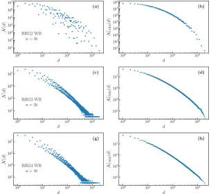
100 ₁₀1 ₁₀2 ₁₀3 ₁₀4 d 100 101 102 N ( d ) (e) Apollonian SR n= 16

100 ₁₀1 ₁₀2 ₁₀3 ₁₀4 d 100 101 102 103 Ncum ( d ) (f )

100 ₁₀1 ₁₀2

d 100 101 102 103 104 N ( d ) (g) Apollonian WR n= 16

100 ₁₀1 ₁₀2

d 100 101 102 103 104 Ncum ( d ) (h)

We plot some examples of some less typical degeneracy distributions in Figure5. These are the 00 and 10 filters applied on a ring, and the SR filter applied to Apollonian networks (which are not degree regular).

2.0 2.5 3.0 3.5 4.0 4.5 5.0

q 0.05 0.10 0.15 0.20 H [ d ] /n (a)

2.0 2.5 3.0 3.5 4.0 4.5 5.0

q 0.1 0.2 0.3 0.4 0.5 0.6 0.7 H [ y ] /n (b) RRG SR SW SR SWB SR cages SR torus SR RRG WR SW WR SWB WR cages WR torus WR

2 3 4 5

q 1.2 1.4 1.6 1.8 2.0 n p d D ( n ) (d)

2 3 4 5

q 1.5 1.6 1.7 1.8 1.9 2.0 n p M ( n ) (e)

2 3 4 5

q 1.4 1.6 1.8 n p N (1 ,n ) (f )

2 3 4 5

q 102 103 104 D ( n ) (c)

n= 30

Figure 6. Dependence of key observables related to the degeneracy distribution on graph degree q. (a) The relevance entropyH[d]scaled by system sizen. (b) ResolutionH[y]. (c) Total number of degeneraciesD(n)forn=30. (d) Thenthroot of the largest degeneracydD(n), which tends tozd. (e) Thenthroot of the number of outputsM(n), tending tozg. (f) Thenthroot of the number of outputs of degeneracy onemN(1,n), tending toza.

In Figure6we represent various quantities of interest as a function of graph degree, for the

different graph families studied. We see that there is a clear separation in results between the two filters.

The weak filter (WR) detects when a node has state 1 while having at least one immediate neighbor with state 0. This neighbour condition is more easily satisfied the larger the number of neighbours

q. Thus for largeq, the number of possible outputsM(n)for the WR filter approaches the number of

possible inputs, 2n. We see in panel (e) that indeed thenthroot ofM(n), which tends tozgfor largen,

approaches 2 for largeq. By the same token, most outputs have a degeneracy of one, so the number of

outputs of degeneracy one,N(1,n)also approaches 2n(zaapproaching 2) for largeq[panel (f)], with

while the largest degeneracydD(n)(whose asymptotic behaviour is given byzd) grows only slowly

withn, [panel (d)]. The resolutionH[y]measures how well the filter distinguishes different inputs,

and as we see in panel (b) of Figure6, and in agreement with the above observations, the resolution

for the weak filter is high. The maximum possible value ofH[y]isnln 2, corresponding to a value of

The correct measure of how informative a sample of the observable variables of a complex system

is about the underlying system is the relevance [8],H[d]. Such sampling is represented in our problem

as the filtering process, and the interactions of the system by the graph structure. The importance of

the relevance is confirmed by our results, as shown in Figure6(a). A higher relevance is measured

in graphs having some randomness in their structure, while deterministic and regular graphs have lower relevance. This is particularly true for the strong filter SR, which produces a significantly higher relevance for random regular graphs (RRG) and rings with random shortcuts (SW), compared with rings with deterministic shortcuts (SWB) and cages. The effect for the WR filter is much less pronounced.

The highest relevance occurs at degreeq=3. The explanation for this is clear. As shown above,

and in [1], smaller filters generally produce higher relevance, as there are more outputs than for larger

filters, except in the extreme limit of perfect reproduction of the input (maximum resolution). Thus

we would expect lower values ofq, which correspond to smaller SR filters, to have higher relevance.

Meanwhile, and opposing this trend, graphs of degreeq =2 are necessarily either rings or sets of

rings, which thus have a (nearly) deterministic structure and suffer a penalty in relevance. Notice

also the similarity of the degeneracy distributions forq=2 in Figures3andA1. As can be seen in

the figure, the reduction in relevance in moving fromq=3 toq=2 due to this regularity outweighs

the expected increase due to the filter being smaller. To put it another way, the maximum relevance

occurs at the smallest value ofqfor which the graph is non deterministic. This echoes our finding for

filters on rings, for which the maximum relevance is found for the shortest filter which doesn’t trivially

reproduce the input [1]. We show the degeneracy ditribution forq=3 for a deterministic graph in

Figure4, and for a random graph in Figure3.

For the SR filter, in contrast to the weak filter, there is significant degeneracy of the outputs. The number of outputs is significantly less than the number of inputs, as is the number of outputs with degeneracy one. Similarly, the resolution is small for the SR filter, for all graph families, and decreases

withq. The largest degeneracy,dD, on the other hand, does become very large. In the limit of largeq, a

large fraction of possible outputs give the same single output (all zeroes). In Figure6(c), the behaviour

of the number of degeneracies,D(n)noticeably mirrors that of the relevance,H[d]. Note that data

points for random graphs are averaged over several realisations of the graph.

In Table2we list the key degeneracy distribution statistics for the SR filter, for all families of

graphs studied. Corresponding results for the WR filter may be found in TableA1. In addition to

representing the data highlighted in Figure6in the quantitative form, these tables demonstrate the

size effects with exponentially rapid convergence to the infinitenlimit. In this work, we are mainly

interested in regular graphs (graphs where nodes have a uniform degree), because we can better isolate the effects of varying the graph’s degree. Nevertheless, for the sake of completeness, we also

present results for a few examples of non-regular graphs, namely Apollonian networks. In Tables2

andA1, each group of rows delimited by horizontal lines represents a different class of graphs. The

four classes at the top of the tables, namely Apollonian networks, cage graphs, square lattices with periodic boundary conditions (torus), rings with deterministic shortcuts, are deterministic graphs, while the two remaining classes represent random models, namely random regular graphs, and rings with random shortcuts. The numbers presented for the random models result from averaging over 10 realizations sampled uniformly at random.

We include results for graphs of several sizes for each type of graph. This allows one to see

the convergence of values with increasingn. Within the set of consecutive rows of each class, the

graphs are ordered by ascending degree, then by ascending number of nodes. The exception to this organization is the two first rows, which are for the non-regular Apollonian networks. All of these

Table 2. Important values for the degeneracy distribution resulting from applying the strong rule (SR) filter to various graphs. The numbers pn M(n), pn dD(n)and n

p

N(1,n)approximatezg,zdandza respectively. We also give the relevance per nodeH[d]/nand the resolution per nodeH[y]/n. Numbers for RRG(q) and SW(q) were obtained by averaging over 10 random realizations.

graph n pn M(n) pn _d

D(n) n p

N(1,n) H[d]/n H[y]/n

Apollonian 2 7 1.47236 1.94420 1.40854 0.08504 0.12919 Apollonian 3 16 1.52380 1.94596 1.49013 0.08148 0.13005

(3,5)-cage 10 1.54199 1.88916 1.42694 0.10463 0.22185 (3,6)-cage 14 1.54904 1.88549 1.46952 0.09741 0.22302 (3,7)-cage 24 1.54516 1.88688 1.42191 0.12412 0.22268 (3,8)-cage 30 1.54618 1.88722 1.44630 0.08763 0.22254 (4,5)-cage 19 1.48991 1.94458 1.37494 0.08094 0.13458 (4,6)-cage 26 1.50129 1.94386 1.44997 0.05243 0.13497 (5,5)-cage 1 30 1.44928 1.97192 1.34932 0.04164 0.07890 (5,5)-cage 2 30 1.44984 1.97191 1.35558 0.04602 0.07891 (5,5)-cage 3 30 1.44954 1.97192 1.35543 0.04201 0.07890 (5,5)-cage 4 30 1.44964 1.97191 1.35280 0.05264 0.07891

torus 3×3 9 1.47967 1.94480 1.42350 0.07165 0.13112 torus 4×4 16 1.51160 1.94843 1.46895 0.06205 0.13043 torus 5×5 25 1.50066 1.94752 1.41779 0.05857 0.13132 torus 6×5 30 1.50206 1.94754 1.42286 0.06159 0.13131 torus 10×3 30 1.48922 1.94678 1.39796 0.05933 0.13100 torus 8×4 32 1.50701 1.94785 1.44980 0.06251 0.13096 torus 6×6 36 1.50405 1.94756 1.44490 0.05890 0.13130

SWB(3) 10 1.55564 1.89336 1.48457 0.10987 0.21539 SWB(3) 20 1.55376 1.89450 1.46394 0.09850 0.21540 SWB(3) 30 1.55377 1.89450 1.46573 0.10256 0.21541 SWB(4) 12 1.48818 1.94653 1.40063 0.07107 0.13103 SWB(4) 21 1.48924 1.94678 1.39802 0.06401 0.13100 SWB(4) 30 1.48922 1.94678 1.39797 0.06211 0.13100 SWB(5) 12 1.43618 1.97359 1.32007 0.04433 0.07602 SWB(5) 20 1.43469 1.97223 1.31634 0.03927 0.07765 SWB(5) 32 1.43463 1.97225 1.31607 0.03597 0.07765

RRG(2) 10 1.55934 1.77122 1.41900 0.15869 0.32044 RRG(2) 20 1.60061 1.76297 1.45744 0.16195 0.33977 RRG(2) 30 1.61251 1.75289 1.46125 0.16997 0.35053 RRG(3) 10 1.49614 1.87903 1.30837 0.17514 0.21708 RRG(3) 20 1.52503 1.87847 1.37793 0.20373 0.22357 RRG(3) 30 1.54129 1.87706 1.41134 0.21442 0.22868 RRG(4) 10 1.44023 1.93770 1.30201 0.11648 0.13463 RRG(4) 20 1.48205 1.93399 1.36490 0.14077 0.14659 RRG(4) 30 1.48439 1.93797 1.37705 0.13959 0.14166 RRG(5) 10 1.41641 1.95111 1.27098 0.10038 0.11042 RRG(5) 20 1.42488 1.96513 1.30706 0.08722 0.08896 RRG(5) 30 1.43068 1.96825 1.31653 0.08344 0.08393

SW(3) 10 1.55356 1.87107 1.43216 0.16610 0.23788 SW(3) 20 1.55998 1.86334 1.43951 0.22050 0.24702 SW(3) 30 1.54842 1.88077 1.43167 0.21643 0.22839 SW(4) 10 1.47637 1.91449 1.33514 0.14321 0.16987 SW(4) 20 1.49157 1.93385 1.38141 0.14235 0.14885 SW(4) 30 1.49811 1.93505 1.39764 0.14519 0.14804 SW(5) 10 1.43017 1.95045 1.29919 0.09802 0.11240 SW(5) 20 1.44575 1.95995 1.33955 0.09722 0.09962 SW(5) 30 1.45251 1.96562 1.35962 0.08951 0.09047

For fully connected graphs, both the strong and the weak rules produce trivial output and

and all other inputsxj6=i=0. So, when there is a 1 in the output string, we haveyi=xi. There arenof

these outputs, and their degeneracy is 1. Since, there can be no more than a single 1 in the output string,

the only other possible output is a string ofnzeros, which has degeneracy 2n−n. In this case there are

only two degeneracies in the degree distributiond1 =1 andd2 =2n−n, and their frequencies are

N(d1,n) =n, andN(d2,n) =1, respectively.

On a fully connected graph under the weak rule, for an output nodeyi to be 1, it is enough to

havexi =1 and just one other inputxj6=i =0. Therefore, when one or more of the inputsxiis 0 the

output is equal to the input. The only situation in which the output does not match the input is for an input string of all 1’s, in which case the output is a strings of 0’s. The weak rule also produces only

two degeneraciesd1=1 andd2=2, with frequenciesN(d1,n) =2n−2, andN(d2,n) =1.

It is worth noticing the relation with the class of cage graphs, which we have studied here:

(q, 3)-cage graphs are fully connected graphs withq+1 nodes, while(q, 4)-cages are bipartite graphs

with two fully connected layers ofqnodes each. Bipartite graphs with two fully connected layers of

the same size also result in trivial degeneracy distributions in both the strong and weak rules. With the

strong rule applied to such a bipartite graph, for an outputyito be 1 we must have all inputs in the

opposite layer to bexi=0. Conversely, when one input of one of the layers isxi =1 all the outputs of

the other layer are 0. So, when all the input digits of one of the layers are all equal to 0 the outputs

equal the inputs,yi =xi, and when there are 1’s in both layers of the input, the output is all 0’s. In

this case the degeneracy distribution also contains just two degeneracies,d1=1 andd2=2n−2n/2+1,

with frequenciesN(d1,n) =2n/2+1andN(d2,n) =1, respectively (notice there aren/2 nodes in each

layer). With the weak rule applied to symmetrical fully connected bipartite graphs, for an outputyito

be 1 it is enough to have just onexi =0 in the opposite layer. Therefore, all inputs with at least a 0 in

each layer produce an outputyi=xi. All inputs with at least one 0 in layerαand only 1’s in layerβ

produce an output consisting of all 0’s in layerαand all 1’s in layerβ. Finally, if the input contains no

0’s in either layer, the output isyi =0 for alli. Therefore, we haved1=1,d2=2, andd3=2n/2−1,

with frequenciesN(d1,n) =2n−2n/2−1,N(d2,n) =1, andN(d3,n) =1, respectively.

From the trivial degeneracy distribution of these examples of graphs, i.e., fully connected and bipartite fully connected, we see that the entropies approach trivial limits for large system sizes.

Namely, for the strong rule, using Eqs. (1) and (2) for the output and degeneracy entropies, respectively,

we see the in both types of graphsH[y]andH[d]both approach 0, since the distribution is dominated

by a single degeneracyd∼=2nwithN(d,n) =1. With the weak rule,the entropyH[y]/napproaches

ln 2=0.693. . . andH[d]approaches 0. In general, we expect that the entropies approach these limits

was we increase the degree of the graphs generated by any model. Interestingly, this effect is already

quite visible in Tables2andA1, when we compare the values of the entropy for different degrees

within each class of graphs, even for degrees up to only 5.

3. Discussion

In Ref. [1] we introduced a simple filtering problem which produces a rich and complex

distribution of output degeneracies. The input is a cyclic sequence of zeroes and ones (a ring), and the process outputs a one in any position where a particular short pattern occurs, and a zero otherwise. The tractability of the problem means that we are able to give the complete degeneracy distribution, for the set of all possible inputs, up to relatively large system sizes.

three key features of the degeneracy distribution: the largest degeneracydD(n), the number of distinct

outputsM(n)and the number of outputs having degeneracy one,N(1,n)behave asz_dn,zn_g andzn_a,

respectively, where the three numberszd,zgandzatake values from 1 to 2 depending on the graph

and the filter. We find precise values for these three numbers for all the graphs studied.

The two filter examples used give quite different results, and have different behaviour with

respect to graph degree. The key results are summarised by our main figure, Figure6. The weak rule

filter, WR, is only weakly sensitive to the neighborhood of a node, and hence the structure of the graph. For large degree, it almost always produces an output matching the input. Thus the WR filter produces large values for the ouput entropy, called the resolution, and small values for the degeneracy entropy, the relevance.

The strong rule filter, SR, on the other hand, imposes a condition on all the neighbours of the node where the filter is applied. This produces a much larger relevance (which is a measure of the informativeness of the filtering process) in random graphs, but much lower resolution, as the number of unique outputs is restricted. The relevance is largest for the smallest graph degree not equal to two. Deterministically constructed graphs do not demonstrate the same peak in relevance, underlining the importance of this measure for detecting complexity. For larger degree, the condition becomes more

restrictive, so the number of outputs is reduced. The resolution decreases with increasingq, but so

does the relevance. The reason that theq=2 graphs do not give the maximum relevance is that these

graphs necessarily have a highly predictable structure. All nodes lie in one or at most a few rings. One may observe that the degeneracy distributions and corresponding statistics are very similar for all

families of graphs studied whenq=2. The fact that results are largely determined by degree, indicates

that it should be possible to write a mean field theory for the degeneracy distribution.

Similar complexity is observed in various complex systems, particularly with regard to information processing. In such systems, degeneracy distributions has been shown to be an important

observation of the system. The entropy of this distribution, called the relevance, was shown [8] to be

the relevant measure of complexity, and we showed that our simple problem reproduces many of the important qualitative phenomena observed in such systems. The filtering problem is therefore a highly tractable problem illuminating some of the key features of information processing in more complex systems. The extension of this problem to arbitrary graphs, makes the interactions between nodes more complex, and the analogy with the complex interactions of real complex systems more explicit.

4. Materials and Methods

4.1. Calculation of degeneracy distributions

The distributions shown in Figures2-5,A1andA2, and the numbers presented in the Tables1,

2, andA1and plotted in Figure6were experimentally obtained by considering all 2nconfigurations

of theninput binary variablesxi individually. For a specified filter, or rule, we obtain the output

variablesyicorresponding to each input. From the frequency with which each output configuration

appears, we build the degeneracy distribution.

For the sake of simplicity in the implementation of the computational experiments, we apply

a basic indexing system to the output configurations. We start by initializing an array with 2n

positions populated with zeros, representing the frequency of observation of each output. Then, as

we systematically run through all the possible inputs and calculate the corresponding outputs{yi},

we increment by 1 the value in position∑iyi2i of the array, wherei = 0, 1, . . . ,n−1. In the end

configurations 2n. In the case of rings, a much more efficient algorithm may be used, as described in

Ref. [1].

4.2. Asymptotics of the degeneracy distribution on rings

Here we show how the asymptotic behaviour of the degeneracy distribution may be obtained. We focus on the particular family of filter patterns consisting of a chain of 1s with a 0 at each end. The shortest such pattern is 010. Each member of this set may be indexed by the length of the filter,

w≥3. Each output consists of isolated ones separated by strings of zeroes of various lengths. The

filter pattern lengthwdetermines the minimum number of zeroes,w−2, between each one.

Forw=3, chains of three or fewer zeroes in the output can only be produced in one way. Thus

outputs containing only such chains of zeroes have degeneracy 1. Possible such output sequences can

be built up out of three kinds of building blocks, 01, 001, and 0001, put together in a ring of lengthn.

We can thus find the number of outputs of degeneracy 1,N(1,n), by counting all possible ways of

building a ring of lengthnout of these blocks. We can do this recursively. For every configuration of

lengthn−2, we can obtain a valid configuration of lengthnby inserting the block 01 to the right, say,

of a particular positioniin the ring. This gives all the configurations of lengthnwith the block 01 to the

right ofi. Doing the same with configurations of lengthn−3 and blocks 001, we get all configurations

with a block 001 to the right of the block ofi. Finally, repeating the procedure for configurations of

lengthn−4 and blocks 0001, gives all configurations with a block 0001 to the right of the block ofi.

Since every block must be 01, 001, or 0001, the union of these three sets is the full set of configurations

of degeneracy 1 in rings ofndigits. Thus, we can write

N(1,n) =N(1,n−2) +N(1,n−3) +N(1,n−4). (4)

Starting from the first few values

N(1, 1)=0, N(1, 2)=2, N(1, 3)=3, N(1, 4)=6, (5)

we could build up the sequence and findN(1,n)for anyn. However it is not necessary to iterate

through all values ofn.

The explicit solution of this linear difference equation (4) can be written in terms of the roots,zi,

of the characteristic equationz4=z2+z+1:

N(1,n) =z1n+z2n+z3n+z4n, (6)

where the coefficients of the powers of the rootszi, all equal to one, are found form the initial condition,

Eq. (5). The rootz1≡za =1.46557... determines the largenasymptotics ofN(1,n).

Forw≥4, it becomes possible for there to be chains of ones in the input that are shorter than that

in the filter pattern. This means that only sequences ofw−2 orw−1 zeroes in the output are not

degenerate. Any sequence ofwor more zeroes in the output can be produced in more than one way.

One may therefore extend an input of degeneracy 1 only by inserting blocks of lengthw−1 andw.

Hence the recursion forN(1,n)becomes

N(1,n) =N(1,n−w+1) +N(1,n−w). (7)

The corresponding characteristic equation is

zw=z+1. (8)

For largen, then,

Wherezacorresponds to the dominant solution of Eq. (8).

The total number of possible outputs may be derived in a similar way. The presence of a 1 at a

given position in the output corresponds uniquely towfixed digits at the same position in the input.

Any degeneracy therefore arises in the parts of the input corresponding to strings of zeroes in the

output. The total number of possible outputs,M(n), is then the number of ways of arranging isolated

ones in a chain of lengthn, subject to this constraint. For every output of lengthn−1, we can create

an output of lengthnby inserting an additional 0. The same is not true for the digit 1, however.

Any 1 in the output must be accompanied by a sequence ofw−2 zeroes. We can account for this

condition precisely by inserting the sequence 10w−2into any valid output of lengthn−(w−1)in a

position immediately following a sequence ofw−2 zeroes (at least one such sequence must exist).

ThusM(n) =M(n−1) +M(n−w+1), with initial conditionsM(n=w) =2,M(n<w) =1. The

elements of the sequence may be written in terms of the roots of the characteristic equation [12–14]

zw−1=zw−2+1. (10)

Thenzgcorresponds to the largest root of this equation. We list values for various filter lengths (as

well as for some other filter patterns) in Table1.

The entire degeneracy distribution may be built up by considering chains of zeroes of different lengths in the output, and the number of different possible corresponding sections of the input. Let an

output withm≥1 ones containmstrings of zeroes with lengths`<sub>1</sub>,`₂, ...,`m. Then the degeneracy of

this output equals

d= m

∏

i=1

˜

d(`_i). (11)

Here ˜d(`)is the number of input strings of length`, having the first and last digits 0, that generate

an output string of`zeroes. This number plays an important role in our problem, similar to prime

numbers in number theory, so we call the ˜d(`)prime degeneracies. Suppose that the output containsµ`

strings of zeroes of length`,`=w−2,w−1,w, ..., where

m+

∑

`≥w−2

`µ<sub>`</sub>=n. (12)

Then Eq. (11) may be rewritten

d=

∏

`≥w−2

[d(˜`)]µ` ₍₁₃₎

form≥1.

The prime degeneracies ˜d(`)can be obtained recursively by taking into account three points:

(i) Relevant input configurations of length`are obtained by inserting 0 or 1 into each relevant

configuration of length`₋1 between the first and second positions of the sequence. (Recall that the

first and last positions of the input sequence are fixed to 0.)

(ii) Input strings of length`beginning and/or ending with 01w−20 are irrelevant, and so they

should be removed from the set generated at the previous step. These configurations can be obtained

by inserting thew−1 digits 1w−20 into each relevant input string of length`−w+1 between its first

and second positions.

(iii) Finally, there exist input strings, compatible with the output string of`zeroes, that cannot be

obtained by inserting a single digit into relevant input strings of length`−1 between their first and

second positions. These are the input strings of length`beginning with 01w−10 (i.e. a string of ones

one digit longer than in the filter). These inputs can be obtained by inserting 1w−10 into each relevant

Following these rules, the degeneracy of a string of`zeroes at the output, prime degeneracy ˜d(`), can be written recursively as a linear difference equation:

˜

d(`) =2 ˜d(`₋1)−_d(˜ `<sub>−</sub>w+1) +d(˜ `₋w) (14)

with the initial condition ˜d(1) = d(˜2) = 1, ˜d(`) = 2`−2for 3 ≤ ` < wandd(w) = 2w−2−1. The

solution of Eq. (14) may be explicitly expressed in terms of the complex roots of the characteristic

equation

zw =2zw−1−z+1. (15)

giving

˜

d(`) =C1z1`+C2z2`+C3z3`+...+Cwzw`. (16)

The largest real root of Eq. (15),z1, say, dominates for large`, and we identify it aszd:

˜

d(`)∼=C1z`d. (17)

The case of the periodic output of lengthnwith all digits 0 has to be considered separately.

Consider one digit of the input, at an arbitrary position. The number of input configurations where this

digit is 0 and the resulting output has only zeroes is given by ˜d(n+1), because the periodicity of the

input means that this digit 0 plays the role of both first and last digit of the configurations of a string

ofn+1 digits. If the digit is 1, then the number of input configurations equals 1+∑i6=w−2id(n˜ −i),

where the sum overiaccounts for the configurations where the digit is in a group oficonsecutive ones

whose length is notw−2, plus one configuration with all input digits equal to 1. Thus the degeneracy

of the output with all zeroes is given by

dD(n) =1+d(n˜ +1) + n−1

∑

i=1;i6=w−2

id(n˜ −i), (18)

which is the largest possible degeneracy of an output of a given length. Applying the recursion relation

for prime degeneracies ˜d, Eq. (14) to the terms on the right-hand side of Eq. (18) we find that the

largest degeneracydD(n)satisfies the same difference equation as Eq. (14) though with different initial

condition

dD(n) =2dD(n−1)−dD(n−w+1) +dD(n−w) (19)

with the initial conditiondD(n) = 2nforn < w, anddD(w) = 2w−w. For largen, the solution is

dominated by a single solution,

dD(n)∼=znd. (20)

Author Contributions: All authors contributed equally substantially in all parts and aspects of the work.

Funding: This work was developed within the scope of the project i3N, UIDB/50025/2020 & UIDP/50025/2020, financed by national funds through the FCT/MEC. This work was also supported by National Funds through FCT, I. P. Project No. IF/00726/2015. R. A. d. C. acknowledges the FCT Grant No. CEECIND/04697/2017.

Conflicts of Interest:The authors declare no conflict of interest.

Appendix A Further results for the weak rule filter

100 ₁₀1 ₁₀2 ₁₀3 d 100 101 102 103 104 105 106 107 N ( d ) (a) ring WR n= 30

100 ₁₀1 ₁₀2 ₁₀3

d 101 103 105 107 Ncum ( d ) (b)

100 ₁₀1 ₁₀2 ₁₀3 ₁₀4

d 101 103 105 107 N ( d ) (c) (3,8)-cage WR

100 ₁₀1 ₁₀2 ₁₀3 ₁₀4

d 101 103 105 107 Ncum ( d ) (d)

100 ₁₀1 ₁₀2 ₁₀3

d 101 102 103 104 105 106 107 108 N ( d ) (e)

torus 6×5 WR

100 ₁₀1 ₁₀2 ₁₀3

d 102 104 106 108 Ncum ( d ) (f )

Figure A1.Degeneracy distributions (left) and cumulative degeneracy distributions (right) for outputs of the WR filter on selected deterministic graphs of degree 2 (a,b) 3 (c,d) and 4 (e,f).

100 ₁₀1 ₁₀2 ₁₀3

d 101 102 103 104 105 106 107 N ( d ) (a) RRG2 WR n= 30

100 ₁₀1 ₁₀2 ₁₀3

d 101 102 103 104 105 106 107 108 Ncum ( d ) (b)

100 ₁₀1 ₁₀2 ₁₀3

d 101 103 105 107 N ( d ) (c) RRG3 WR n= 30

100 ₁₀1 ₁₀2 ₁₀3

d 101 103 105 107 Ncum ( d ) (d)

100 ₁₀1 ₁₀2 ₁₀3

d 101 103 105 107 N ( d ) (g) RRG4 WR n= 30

100 ₁₀1 ₁₀2 ₁₀3

d 101 103 105 107 Ncum ( d ) (h)

Table A1. Important values for the degeneracy distribution resulting from applying the weak rule (WR) filter to various graphs. The numbers pn M(n), pn dD(n)and n

p

N(1,n)approximatezg,zdandza respectively. We also give the relevance per nodeH[d]/nand the resolution per nodeH[y]/n. Numbers for RRG(q) and SW(q) were obtained by averaging over 10 random realizations.

graph n pn M(n) pn _d

D(n) n p

N(1,n) H[d]/n H[y]/n

Apollonian 2 7 1.95461 1.21901 1.91660 0.11519 0.66045 Apollonian 3 16 1.94788 1.43435 1.91189 0.09594 0.64711

(3,5)-cage 10 1.91202 1.21481 1.84295 0.13705 0.62974 (3,6)-cage 14 1.91394 1.34590 1.83757 0.12271 0.63149 (3,7)-cage 24 1.91348 1.25055 1.83511 0.11462 0.63259 (3,8)-cage 30 1.91330 1.34897 1.83337 0.10559 0.63275 (4,5)-cage 19 1.95248 1.21101 1.91027 0.08217 0.65878 (4,6)-cage 26 1.95322 1.37995 1.91085 0.07188 0.65902 (5,5)-cage 1 30 1.97461 1.16392 1.95220 0.04494 0.67453 (5,5)-cage 2 30 1.97461 1.18854 1.95219 0.04495 0.67453 (5,5)-cage 3 30 1.97461 1.21540 1.95220 0.04496 0.67453 (5,5)-cage 4 30 1.97461 1.17585 1.95220 0.04495 0.67453

torus 3×3 9 1.95698 1.16653 1.92324 0.10088 0.66192 torus 4×4 16 1.95546 1.38485 1.92191 0.09024 0.65777 torus 5×5 25 1.95475 1.21993 1.91904 0.08076 0.65828 torus 6×5 30 1.95475 1.28517 1.91898 0.07568 0.65831 torus 10×3 30 1.95626 1.22522 1.91924 0.07072 0.66127 torus 8×4 32 1.95510 1.38392 1.91932 0.07475 0.65813 torus 6×6 36 1.95475 1.38400 1.91883 0.07034 0.65833

SWB(3) 10 1.91492 1.35588 1.85212 0.14568 0.62873 SWB(3) 20 1.91523 1.30100 1.84849 0.12731 0.62956 SWB(3) 30 1.91523 1.35620 1.84851 0.11281 0.62956 SWB(4) 12 1.95603 1.17605 1.91983 0.09152 0.66087 SWB(4) 21 1.95626 1.21231 1.91923 0.08079 0.66127 SWB(4) 30 1.95626 1.20790 1.91924 0.07071 0.66127 SWB(5) 12 1.97929 1.17605 1.96131 0.05848 0.67803 SWB(5) 20 1.97927 1.16442 1.96025 0.04881 0.67840 SWB(5) 32 1.97927 1.14893 1.96021 0.04144 0.67842

RRG(2) 10 1.76075 1.33214 1.62827 0.16029 0.53010 RRG(2) 20 1.81141 1.29593 1.65746 0.14345 0.56553 RRG(2) 30 1.83115 1.27447 1.67090 0.11728 0.58305 RRG(3) 10 1.86350 1.31014 1.73760 0.18497 0.59914 RRG(3) 20 1.88987 1.28690 1.78608 0.13766 0.61721 RRG(3) 30 1.89895 1.27941 1.80483 0.11537 0.62310 RRG(4) 10 1.92754 1.24293 1.86647 0.13602 0.64106 RRG(4) 20 1.93917 1.25076 1.88272 0.09610 0.65019 RRG(4) 30 1.94507 1.25247 1.89654 0.07819 0.65347 RRG(5) 10 1.93764 1.26982 1.88340 0.12318 0.64808 RRG(5) 20 1.95952 1.23790 1.92369 0.07520 0.66371 RRG(5) 30 1.96616 1.22872 1.93641 0.05720 0.66839

References

1. Baxter, G.; da Costa, R.; Dorogovtsev, S.; Mendes, J. Complex distributions emerging in filtering and compression.Physical Review X2020,10, 011074.

2. Song, J.; Marsili, M.; Jo, J. Emergence and relevance of criticality in deep learning. arXiv preprint arXiv:1710.113242017.

3. Baek, S.K.; Bernhardsson, S.; Minnhagen, P. Zipf’s law unzipped. New Journal of Physics2011,13, 043004. 4. Hartmann, A.K.; Weigt, M.Phase Transitions in Combinatorial Optimization Problems; Whiley-VCH, Weinheim,

2005.

5. Mézard, M.; Parisi, G.; Virasoro, M.Spin Glass Theory and Beyond: An Introduction to the Replica Method and Its Applications; World Scientific, Singapore, 1987.

6. Keskar, N.S.; Mudigere, D.; Nocedal, J.; Smelyanskiy, M.; Tang, P.T.P. On large-batch training for deep learning: Generalization gap and sharp minima. arXiv preprint arXiv:1609.048362016.

7. Dorogovtsev, S.N.; Goltsev, A.V.; Mendes, J.F.F. Critical phenomena in complex networks. Rev. Mod. Phys. 2008,80, 1275. doi:10.1103/RevModPhys.80.1275.

8. Cubero, R.J.; Jo, J.; Marsili, M.; Roudi, Y.; Song, J. Minimally sufficient representations, maximally informative samples and Zipf’s law. arXiv preprint arXiv:1808.002492018.

9. Marsili, M.; Mastromatteo, I.; Roudi, Y. On sampling and modeling complex systems. J. Stat. Mech.: Theory and Experiment2013,2013, P09003.

10. Cubero, R.; Marsili, M.; Roudi, Y. Minimum Description Length codes are critical. Entropy2018,20, 755. 11. Meringer, M. Fast generation of regular graphs and construction of cages. Journal of Graph Theory1999,

30, 137.

12. Hoggatt Jr., V.E.Fibonacci and Lucas Numbers; Houghton Mifflin, Boston, MA, 1969.

13. Graham, R.L.; Knuth, D.E.; Patashnik, O.; Liu, S.Concrete Mathematics: A Foundation for Computer Science; Addison-Wesley Publishing Company, Reading, Massachusetts, 1994.