Discrete and Continuous Optimization for Motion Estimation

(1)

Publicly Accessible Penn Dissertations

1-1-2015

Discrete and Continuous Optimization for Motion

Estimation

Ryan Kennedy

University of Pennsylvania, [email protected]

Follow this and additional works at:http://repository.upenn.edu/edissertations Part of theComputer Sciences Commons

This paper is posted at ScholarlyCommons.http://repository.upenn.edu/edissertations/1075

For more information, please [email protected]. Recommended Citation

Kennedy, Ryan, "Discrete and Continuous Optimization for Motion Estimation" (2015).Publicly Accessible Penn Dissertations. 1075.

(2)

Abstract

The study of motion estimation reaches back decades and has become one of the central topics of research in computer vision. Even so, there are situations where current approaches fail, such as when there are extreme lighting variations, significant occlusions, or very large motions. In this thesis, we propose several approaches to address these issues. First, we propose a novel continuous optimization framework for estimating optical flow based on a decomposition of the image domain into triangular facets. We show how this allows for occlusions to be easily and naturally handled within our optimization framework without any post-processing. We also show that a triangular decomposition enables us to use a direct Cholesky decomposition to solve the resulting linear systems by reducing its memory requirements. Second, we introduce a simple method for incorporating additional temporal information into optical flow using "inertial estimates" of the flow, which leads to a significant reduction in error. We evaluate our methods on several datasets and achieve state-of-the-art results on MPI-Sintel. Finally, we introduce a discrete optimization framework for optical flow

computation. Discrete approaches have generally been avoided in optical flow because of the relatively large label space that makes them computationally expensive. In our approach, we use recent advances in image segmentation to build a tree-structured graphical model that conforms to the image content. We show how the optimal solution to these discrete optical flow problems can be computed efficiently by making use of optimization methods from the object recognition literature, even for large images with hundreds of thousands of labels.

Degree Type

Dissertation

Degree Name

Doctor of Philosophy (PhD)

Graduate Group

Computer and Information Science

First Advisor

Camillo J. Taylor

Keywords

Computer Vision, Motion, Optical Flow

Subject Categories

Computer Sciences

(3)

Ryan Kennedy

A DISSERTATION

in

Computer and Information Science

Presented to the Faculties of the University of Pennsylvania

in

Partial Fulfillment of the Requirements for the

Degree of Doctor of Philosophy

2015

Supervisor of Dissertation

Camillo J. Taylor, Professor, Computer and Information Science

Graduate Group Chairperson

Lyle Ungar, Professor, Computer and Information Science

Dissertation Committee

Kostas Daniilidis, Professor, Computer and Information Science

Jean Gallier, Professor, Computer and Information Science

Jianbo Shi, Professor, Computer and Information Science

(4)

ESTIMATION

COPYRIGHT

2015

(5)

Acknowledgements

This thesis would not exist if not for the help of many people along the way. First,

a sincere thanks to my advisor C.J. Taylor. Working with him then has been

incredibly productive and fun. He seems to always have new ideas that he’s eager

to share and his support in all aspects of my work at Penn has been astounding.

He has my sincere gratitude for all his help.

I’d also like to thank Jianbo Shi, with whom I worked for several years after

joining Penn. Before starting grad school, I had no knowledge of computer vision

whatsoever, and Jianbo was able to show me how interesting computer vision really

is. He has been a fantastic teacher and I owe much of my success in computer

vision to what he taught me.

Thanks as well to Kostas Daniilidis, with whom I worked with for a time and

who has been supportive all along, and is also the head of my thesis committee.

I’d also like to thank Jean Gallier, with whom I worked with on a paper during

my first year at Penn and who is also a member of my thesis committee. Jean is

certainly one of the most fun people I have had to chance to work with, with his

unique and wonderful combination of mathematical rigour and silly jokes. Finally,

thanks also to the external member of my thesis committee, Rick Szeliski, for his

time and help.

I’ve also had the great opportunity to collaborate with Laura Balazano, now at

the University of Michigan, and I have learned a huge amount working with her.

I would also not even be at Penn were it not for the initial help of Lyle Ungar and

my undergraduate advisor Rob Knight in my admission. There are many others

(6)

for their huge administrative help, Vijay Kumar for briefly working with me at

the start of my program, and Ben Taskar and Mitch Marcus for whom I was a

teaching assistant.

I also would like to thank my colleagues, including David, Katerina, Cody, Weiyu,

Kosta, and many others, who made my time at Penn very enjoyable. Finally,

(7)

ABSTRACT

DISCRETE AND CONTINUOUS OPTIMIZATION FOR MOTION

ESTIMATION

Ryan Kennedy

Camillo J. Taylor

The study of motion estimation reaches back decades and has become one of

the central topics of research in computer vision. Even so, there are situations

where current approaches fail, such as when there are extreme lighting variations,

significant occlusions, or very large motions. In this thesis, we propose several

approaches to address these issues. First, we propose a novel continuous

opti-mization framework for estimating optical flow based on a decomposition of the

image domain into triangular facets. We show how this allows for occlusions to

be easily and naturally handled within our optimization framework without any

post-processing. We also show that a triangular decomposition enables us to use

a direct Cholesky decomposition to solve the resulting linear systems by reducing

its memory requirements. Second, we introduce a simple method for incorporating

additional temporal information into optical flow using “inertial estimates” of the

flow, which leads to a significant reduction in error. We evaluate our methods on

several datasets and achieve state-of-the-art results on MPI-Sintel. Finally, we

in-troduce a discrete optimization framework for optical flow computation. Discrete

approaches have generally been avoided in optical flow because of the relatively

large label space that makes them computationally expensive. In our approach,

we use recent advances in image segmentation to build a tree-structured graphical

model that conforms to the image content. We show how the optimal solution to

(8)

optimization methods from the object recognition literature, even for large images

(9)

List of Tables

3.1 Effect of graph and re-ordering on Cholesky solver . . . 64

4.1 Endpoinr error on the Middlebury test dataset. . . 77

4.2 Results on the MPI-Sintel test set. . . 78

4.3 Results on the KITTI test set . . . 80

4.4 Results on a validation set from KITTI . . . 81

5.1 Endpoint error on Middlebury . . . 101

5.2 Evaluation on the Final training dataset of MPI-Sintel. The use if inertial estimates improves results. . . 103

5.3 Evaluation on the Final test dataset of MPI-Sintel. We report end-point error for all pixels, and also based on the groundtruth speed.. 105

5.4 Effect of segmentation error on MPI-Sintel. . . 107

(13)

List of Figures

1.1 Scenes where motion is an important cue. . . 2

1.2 The setup of the cylinder used in Ullman’s experiment . . . 3

1.3 The barber’s pole illusion. . . 4

1.4 An example of the optical flow problem. . . 5

1.5 An example of the optical flow problem. . . 11

1.6 A depiction of the aperture problem. . . 14

2.1 Graphical depiction of the aperture problem . . . 19

2.2 Example of the difficulties that occlusion causes. . . 30

2.3 A situation where muti-frame optical flow is essential . . . 32

2.4 4- and 8-connected MRF neighborhoods. . . 35

2.5 Examples from optical flow datasets. . . 43

3.1 A triangulated section of an image. . . 46

3.2 Matching errors are well-fit by a Cauchy distribution . . . 51

3.3 Depiction of our occlusion term. . . 55

3.4 Examples of our occlusion estimation on MPI-Sintel. . . 56

3.5 Comparison of time taken by linear solvers for optical flow. . . 68

3.6 Effect of linear solvers on mean endpoint error . . . 69

4.1 Inertial flow estimates used in multi-frame fusion . . . 72

4.2 Examples of our multi-frame fusion on the MPI-Sintel training set . 74 4.3 Examples of our multi-frame fusion on the KITTI training dataset . 75 4.4 Violation of the assumption of inertial estimates on MPI-Sintel . . . 79

4.5 Qualitative results on Tears of Steel . . . 82

5.1 Depiction of our segmentation-based hierarchical model . . . 85

5.2 Estimated optical flow on two images from the Middlebury dataset 86 5.3 Distribution of offsets in MPI-Sintel. . . 89

5.4 Compressing the Voronoi diagram . . . 97

5.5 Depiction of our multi-frame term . . . 99

5.6 Results on the Middlebury training set . . . 102

5.7 Results on several images from the Final training dataset of MPI-Sintel. . . 104

5.8 Example images show the effect of segmentation on optical flow results on MPI-Sintel using HCOF . . . 106

(14)

5.10 Results on the synthetic dataset. . . 108

5.11 An example of a result from the Tracking dataset. . . 110

5.12 Effect of sub-pixel localization on a portion of the RubberWhale image from the Middlebury dataset. . . 114

5.13 Results on the Middlebury training set . . . 115

A.1 Examples of our multi-frame fusion on the MPI-Sintel training set . 120

A.5 Examples of our multi-frame fusion on the KITTI training dataset . 124

(15)

1

Introduction

In one of the more iconic scenes from the filmJurassic Park, two children Lex and Tim Murphy are trapped in their jeep during a rainstorm while aTyrannosaurus rex attacks them. Coming to their rescue, Dr. Grant runs to the jeep and tells them to stay still: “Don’t move. He can’t see us if we don’t move.” To the viewers’ relief, the plan works, and the fearsome dinosaur is unable to locate them despite

being just a few feet away.

Of course, the idea that T. Rex was unable to separate people form the back-ground without the aid of motion is simply untrue. In fact, theT. Rex likely had exceptional vision (Stevens, 2006), although this would have resulted in a much

shorter movie with a less happy ending. Even so, it is certainly true that motion

can provide essential information for our understanding of the visual world. A

similar situation to that ofJurassic Park can be seen through the camouflage that animals use in nature. Consider, for example, Figure 1.1a, which depicts a lion

hidden in tall grass as it stalks its prey. From static visual information alone, it

may be extremely difficult to tell that the lion is there. In this case, motion can

indeed prove to be an extremely valuable cue for detecting predators. Another

(16)

(a) A lion hiding in the grass. (Dupont, 2014)

(b) A street scene involving

pedestrians. (Wang et al.,2007)

Figure 1.1: Scenes where motion is an important cue. In (A), the tall grass

obscures a lion. Without motion, the lion may be difficult to see. In (B), the motions of the pedestrians are necessary for determining where to walk down the street.

pedestrians are walking down the street. In order for us to walk down the street

ourselves, it is necessary to determine the motion of each person and plan a path

to avoid them. Situations such as this that involve path planning around moving

objects show up in robotics and autonomous driving applications.

Motion can play an essential role for scene understanding even in extremely simple

situations, as was convincingly demonstrated in an experiment by Ullman (Ullman,

1979). In his experiment, Ullman constructed constructed two cylinders that were

invisible aside from a set of random dots on their surfaces. One cylinder was placed

within the other and they were rotated in opposite directions. This setup is shown

in Figure1.2. Only the orthographic projection of the cylinders from the side was

made visible, and so at any point in time the image on the screen appeared to be

just a random collection of dots. However, when the cylinders were rotated, the

(17)

Figure 1.2: The setup of the cylinder used in Ullman’s experiment (Ullman,

1979). Two concentric transparent cylinders rotate in opposite directions. The cylinders are depicted in gray, although they are were not visible in the exper-iment. The random dots on the cylinder appear as just a collection of random dots at a single frame, but as the cylinders rotate the correct object

segmen-tation and 3D structure is perceived. Figure adapted by author from (Ullman,

1979).

put it,

[W]hen the changing projection was viewed, the elements in the motion across the screen were perceived as two rotating cylinders whose shapes and angles of rotation were easily determined. Both the segmentation of the scene into objects and the 3-D interpretation were based in this case on the motion alone, since each single view contained no information concerning the segmentation or the structure.

This demonstration shows that, indeed, motion is a very important cue for

vi-sual perception. Motion aids in our understanding of the structure and semantic

meaning of scenes.

Unfortunately, motion cues can also fool us. Consider the classic barber’s pole

illusion, as shown in Figure 1.3. As the pole spins, our perception is that the

(18)

Figure 1.3: The barber’s pole illusion. As the pole spins around its vertical axis, it appears that the motion of the pole has a vertical component when there is none. The is due to the aperture problem.

around its vertical axis. An illusion of this type demonstrates that, even with

motion, a visual interpretation of a scene can be ambiguous. In this case, the

illusion is caused by the fact that is only possible to estimate local motion that is

perpendicular to an edge, which is known as the aperture problem. In reality, the barber pole could be moving one of many different directions based on our limited

view of it, and our minds choose just one of these interpretations. Thus, the

underlying algorithms that we use to estimate motion – and their associated biases,

both implicit and explicit – play a significant role in our resulting interpretation

of the world.

The barber’s pole illusion also illustrates the difference between the true motion field and the apparent motion oroptical flow of a scene. While the true motion of the pole is a rotation around its vertical axis, the apparent motion is ambiguous

(19)

(a)Image 1 of the Grove2

se-quence.

(b) Image2 of the Grove2

se-quence.

(c)Groundtruth optical flow. (d)Color key for groundtruth optical flow values. Direction is indicated by hue while mag-nitude is indicated by satura-tion of the colors.

Figure 1.4: An example of the optical flow problem, taken from the

Middle-bury dataset (Baker et al.,2011)

is spinning may have a very large motion but impart zero optical flow.

Computa-tionally, images are all that we have access to and so the optical flow of a scene is

all that we can estimate. Its estimation is the topic of this thesis.

An example of optical flow estimation on a real image is shown in Figure 1.4.

Given a sequence of images, the goal of optical flow estimation is to determine the

offset that each pixel in the image at time t moves to at time t+ 1. We display

the estimated flow field using a color image, where the hue at each pixel indicates

(20)

1.1 Applications of Optical Flow

We begin by outlining several concrete applications of optical flow to further

mo-tivate the issues studied in this thesis.

1.1.1 Video interpolation

While a video may be pre-recorded and fixed, in many cases it is desirable to look

at the scene from a viewpoint – in either time or space – that is not captured at any

of the frames of the video. In (Zitnick et al., 2004), a method was proposed that

used motion estimation between a set of cameras to interpolate to novel viewpoints

in the scene. In (Mahajan et al., 2009), a method closely related to optical flow

was used to obtain high-quality interpolation between frames in a single video.

1.1.2 Tracking

Optical flow has an clear application to tracking: if an accurate motion field can

be obtained, then tracking an object can be done just by tracking each associated

point using the estimated flow. Local methods for optical flow have also been used

to directly track individual points (Shi and Tomasi, 1994). Features derived from

flow fields can also be used indirectly as features within a more complex tracking

system, such as for tracking a human pose (Sapp et al., 2011; Fragkiadaki et al.,

(21)

1.1.3 Action recognition

When attempting to estimate the actions that occur in a video, motion can be

an important cue. For example, in (Wang et al.,2011;Bhattacharya, 2013; Fathi

and Rehg,2013), dense motion estimates were used to generate features for action

recognition.

1.1.4 Relationship to stereo correspondence

Optical flow is also closely related to the stereo correspondence problem. In

con-trast to optical flow where two frames are typically of the same scene but separated

in time, stereo uses two images of a scene from the same point in time but different

spatial locations. This results in a slightly different problem, since the scene is

completely rigid with respect to the stereo images and all motion is due to the

camera. For every pixel, the set of possible correspondences in the other image are

no longer the set of all pixels in the other image since the correspondence must lie

on an epipolar line (Szeliski, 2010; Hartley and Zisserman, 2003). If the images

are rectified first (Hartley and Zisserman,2003), then this is equivalent to finding

only the horizontal offset for each pixel, rather than both horizontal and vertical

as is the case for optical flow. In this way, optical flow methods can be applied

directly to the stereo problem as well. However, because the problem is somewhat

different, a different set of algorithms that include the use of discrete optimization

(Boykov et al., 2001; Kolmogorov and Zabih, 2001) or segmentation (Yang et al.,

(22)

1.1.5 Relationship to general image correspondence

Optical flow is also related to the general image correspondence problem. In this

setup, a correspondence is estimated between two semantically similar images

which may not be from the same scene. Because the images may be from different

scenes, color or image intensity are not useful features, and more complex

descrip-tors such as SIFT (Lowe, 2004; Liu et al., 2011) need to be used. The models

for image correspondence may also need to account for difficulties such as scale

changes (Hassner et al., 2012; Kim et al., 2013a), but in general the approach is

similar to that of optical flow (Liu et al.,2011). One particularly useful application

of image correspondence is for label transfer, where labels from one image can be

transfered to another by aligning an image to a pre-labeled database (Liu et al.,

2009). This approach can also be used in medical imaging (Kybic and Unser,

2003) to align a given medical image to a model image in order to analyze it or

detect irregularities.

1.2 Modeling Optical Flow

The basic problem of optical flow can be stated simply: for each pixel in an image,

determine its corresponding location in a subsequent image. To gain tractability

on solving this problem, a set of simplifying assumptions are used to

mathemati-cally formalize the idea of what constitutes a “good” solution. Optical flow models

generally rely on two assumptions about objects within our physical world. First,

it is assumed a physical object maintains a similar appearance through time – at

least over a short time span. Second, it is assumed that physical objects tend to

(23)

correlated; points that are very close to each other in the image are likely to be

part of the same object and have a similar motion due to the motion of that object.

These two assumptions – that objects maintain a similar appearance through time

and that nearby points have correlated motions – will be referred to as the bright-ness constancy assumption and the smoothness assumption. Although the term “brightness constancy” originally comes from models where the images have only

a single, grayscale “brightness” channel, we may refer to this assumption as the

idea that objects have a similar apperance through time, even if that appearance

is measured using color or more complex features.

1.2.1 Brightness Constancy Assumption

The simplest form of brightness constancy states that for grayscale images, two

corresponding pixels have a similar intensity value. This is easily written as a

mathematical constraint, and forms the basis of all optical flow algorithms. In

an ideal situation, this is the only constraint that is needed: each pixel can be

corresponded with its closest match in the next image. However, simple pixel

intensities are often insufficiently discriminative and the optical flow problem is

underconstrained. Instead, more information can be used, such as color or even

more complex features. Additionally, a smoothness assumption can be used as a

regularization in order to impose more structure on the resulting motion fields.

1.2.2 Smoothness Assumption

Due to the coherence of objects in our world, two points near each other in an

(24)

in different ways, and boradly splits algorithms into two categories: local and

global methods. In local algorithms, the smoothness assumption assumes that a separate local parametric model exists to describe the motion of each pixel

indi-vidually. This allows for information to be aggregated over local neighborhoods

in the image. The motion of each pixel is then solved for independently. In

con-trast, global algorithms define a single, global cost function which encodes both

the brightness constancy assumption as well as a penalty for when nearby pixels

have significantly different motion estimates. A global cost function is generally

more difficult to solve since it is often non-convex and cannot be as easily

paral-lelized as local cost functions. However, incorporating information globally, over

the entire image domain, can result in much more accurate solutions. Modern

optimization methods have improved the speed and reliability of global methods,

and the most accurate optical flow algorithms today typically use some form of

global optimization.

1.3 Challenges

The basic brightness constancy and smoothness assumptions are not hard to model

mathematically, and in many cases simple approaches are able to produce

high-quality motion estimates relatively efficiently. However, these basic assumptions

can break down.

1.3.1 Lighting Variation

Lighting variations lead to violations of the brightness constancy assumption. For

(25)

(a) A pair of images from the KITTI dataset (Geiger et al., 2012).

Shadows cause violations of the brighness constancy constraint and low contrast grayscale images make feature matching difficult.

(b)A pair of images from the MPI-Sintel dataset (Butler et al.,2012).

Large motions result in motion blur, making matching difficult.

(c)A pair of images from the MPI-Sintel dataset (Butler et al.,2012).

Large occluded regions have no match in the second frame.

Figure 1.5: An example of the optical flow problem.

image. This is a major problem in, for example, the KITTI dataset as shown in

Figure 1.5a, where a combination of low-contrast grayscale features and outdoor

scenes results in gross violations of brightness constancy. Even when color images

are used, however, differences in lighting can cause significant changes in color.

1.3.2 Imaging and Atmospheric Effects

The imaging process itself is imperfect, and this can lead to violations in brightness

constancy as well. Again, in the KITTI dataset as shown in Figure 1.5a, the

cameras produce only low-contrast grayscale images. In the MPI-Sintel dataset

(26)

as shown in Figure1.5b. A related problem is caused by atmospheric effects, where

fog or glare can prevent the camera from capturing the true color of the object

represented at each pixel.

1.3.3 Occlusions

The brightness constancy assumption has an underlying assumption that each

point in an image has a correct correspondence in the other image. When objects

are occluded, this is no longer the case. Instead, points may go out of frame or

be blocked by an occluding object, and brightness constancy can not possibly be

used in these regions to find an accurate solution. Occlusions also cause problems

for the smoothness assumption. If multiple objects are moving in the same image,

then pairs of pixels on the border between objects or an object and the background

may refer to two completely different positions in 3D space, even though they are

adjacent in the image. The motions of these pixels are no longer correlated, and

assuming that the motion field is smooth across these occlusion boundaries will

give the wrong solution. Figure 1.5c shows a pair of frames exhibiting a large

occluded regions for which no matches are present in the second frame.

1.3.4 Complex Motions

The simplest form of the smoothness assumption simply penalizes adjacent pixels

that have different motions. More complex motions, however, will violate this. For

example, articulated or non-rigid objects – such as a waving flag or a deforming

piece of paper – are penalized by this smoothness constraint. Additionally, even

(27)

parallel to the image plane. This assumption is heavily violated in the KITTI dataset (Geiger et al., 2012), where the camera is mounted to a forward-moving

car and so pixels move significantly more as they are closer to the camera. This

is also seen as a change in scale for objects that move towards or away from the

camera. Large motions can also cause issues for local optimization methods (Brox

and Malik, 2011).

1.3.5 The Aperture Problem

The aperture problem pervades all optical flow datasets, regardless of the type of

image or model used. This problem is demonstrated in Figure 1.6. The problem

is that any region of an image has only a limited view. Consider an image

re-gion that views the center of a textureless, white piece of paper. If the paper is

shifted slightly, the image does not change! In this case, there is no possible way

to determine the motion from that region alone. Similarly, for an image region

centered on a line, only motionsperpendicular to the line can be determined. The aperture problem is commonly seen in barbershop poles (Figure1.3). The

appar-ent motion of a barber pole is exactly the same if the pole is moving vertically or

spinning. Our mind chooses a single interpretation, but the motion is ambiguous.

The aperture problem is especially difficult for local methods, where information

in the image is aggregated over only a small area. Global methods, in contrast, are

able to propogate the motion from areas that are highly-discriminative to those

(28)

Figure 1.6: A depiction of the aperture problem. For a local corner region, the motion of the associated pixel can be reliably matched the second image. However, for non-corner regions, such as those within the rectangle, the motion is ambiguous.

1.3.6 Optimization

A slightly different problem is how a model should be optimized. For example,

the set of possible motions that can be assigned to a pixel can be thought of

as either a continuous or a discrete space, and different methods with different

advantages and disadvantages can be applied depending on the choice. Within

both discrete and continuous approaches, there are a large number of possible

optimization methods: gradient descent, Newton’s method, mean-field methods,

message passing, etc. The choice of optimization methods has expanded and

improved significantly in the last few years, and it depends largely on the choice

of model. There is a tradeoff here as well: more complex models may be more

realistic and more closely relate to the data, but they are often more difficult to

optimize. Any optical flow method must decide where in this tradeoff to position

(29)

1.4 Contributions of this thesis

This thesis provides three main contributions. First, we present a novel optical

flow model which is based on a triangulation of the image domain. The basis of

our model is similar to past approaches in that it involves estimating the motion

of an image by imposing both data and smoothness terms over a discretization

of the image. However, in our model we view the triangles as discrete geometric

pieces over which motion is estimated. We show how this triangulation allows for

occlusions to be directly and naturally incorporated into the optimization problem.

This approach is continuous in nature, and we use Newton’s method to find a local

optimum, which is typically avoided due to computational reasons. In fact, we

show how a triangulated image allows for an exact Cholesky factorization to be

used within Newton’s method by reducing the memory requirements of Cholesky

factorization.

Second, we introduce the idea of inertial estimates of optical flow. Inertial esti-mates are estiesti-mates of image motion that are taken from adjacent frames. These

inertial estimates can be fused using a classifier, resulting in significant

improve-ments in accuracy. This method is a simple, effective approach to using temporal

information from a video sequence. When used together with our triangulated

model, this results in state-of-the-art optical flow estimates on the difficult

MPI-Sintel dataset.

Finally, we present a discrete approach to motion estimation. Discrete

optimiza-tion is frequently used in related domains such as stereo correspondence, and

has the advantage that a near-optimal solution can be found in many situations.

(30)

label space that makes many discrete approaches impractical. We propose a novel

method that combines a hierarchical Markov random field with optimization

tech-niques from the literature on object detection. We show that this problem can

be solved optimally even for label spaces with hundreds of thousands of labels. We also show how this discrete approach allows for inertial estimates to be easily

added, which reduces the runtime requirements for their use.

The outline of this thesis proposal is as follows. In Chapter 2, we review current

methods for optical flow and how they relate to our approach. Our

triangulation-based model is then presented in3. In Chapter 4, inertial estimates are proposed

and we show how they can be fused using a classifier into a single motion estimate.

We also evaluate our triangulation-based model with the inertial estimates, which

results in a state-of-the-art optical flow algorithm. Our discrete approach to optical

flow is then proposed and evaluated in Chapter5. Finally, we conclude in Chapter

(31)

2

Preliminaries and Related Work

In this chapter, we review related work in motion estimation to provide context for

the contributions of this thesis. We begin by presenting a brief outline of a very

common approach to optical flow estimation. We then review modern techniques

and how they differ from this model with a focus on approaches that are related

to the algorithms proposed in subsequent chapters.

2.1 Basic Approach to Optical Flow Estimation

A fundamental assumption made in optical flow is the brightness constancy as-sumption, which says that a pixel’s appearance remains relatively constant

be-tween frames. Formally, let I(x, y, t) be a time-dependent image sequence, such

that our goal is to estimate the motion from I(x, y, t) toI(x, y, t+ 1). The

bright-ness constancy assumption then says that

(32)

where u and v are the estimated horizontal and vertical displacements at each

pixel. Mathematically, we can write this as a constraint

I(x+u, y+v, t+ 1)−I(x, y, t) = 0 (2.2)

or as an`2 penalty [I(x+u, y+v, t)−I(x, y, t)]2.

If we linearize this constraint by taking its first order Taylor expansion around the

current estimate, we have

Ixu+Iyv+It= 0, (2.3)

where Ix, Iy and It are the partial derivatives of I with respect to x, y and t,

respectively. To aid in its interpretation, we rewrite this constraint as

Ix Iy

q I2

x+Iy2     u v    

= q −It I2

x+Iy2

. (2.4)

This constraint is a line, and it says that the displacement vector

u v

is

per-pendicular to the image gradient

Ix Iy

with a projected magnitude of √−It

I2

x+Iy2 in

that direction. This is depicted in Figure 2.1. From the figure, it is clear that the

linearized brightness constancy equation is insufficient to determine the

displace-ment at that pixel uniquely. Indeed, only the component of the flow orthogonal

to the image gradient can be determined. This is a mathematical depiction of the

aperture problem.

Because a single constraint at each pixel leads to an under-constrained system

of equations, it is necessary to impose regularization in order to obtain a unique

(33)

v

u

(Ix, Iy)

−It

√

I2

x+Iy2

Figure 2.1: Graphical depiction of the aperture problem due to the linearized brightness constancy constraint. The standard linearized brightness assumption constraints the displacement vector [u, v] to be on a line perpendicular the image gradient at that point. Thus, the displacement is undefined from only one such equation.

divided into distinct, compact, solid objects and thus pixels that are nearby in the

image likely belong to the same object and have a similar motion. This constraint

was used by Lucas and Kanade (Lucas et al.,1981), who impose the constraint that

the motion field is constant in a small region around each pixel. Then, for each pixel, there are now multiple equation rather than just one. For example, using

a 5×5 neighborhood around each pixel results in 25 equations, still with only 2 unknowns. The linear system is now over-determined, and a least-squares solution

can be found using standard linear solvers. However, this solution is only valid for

small displacements since the brightness constancy equation was linearized, and

so the equations are re-linearized around the new solution estimate. This process

is repeated until convergence.

The Lucas Kanade method works well in many cases, and the local approach

has computational benefits: solving small linear systems can be done extremely

(34)

local nature of this approach makes it useful in other contexts as well, such as

object tracking (Shi and Tomasi,1994), where a dense motion field is not required

and tracking discriminative points on an object can be done independently from

each other. There are, however, drawbacks of this approach. First, the aperture

problem (see Section1.3.5) forces us to use neighborhoods that are sufficiently large

so that they include local texture information. However, larger neighborhoods

also have a greater chance of including irrelevant points that are not part of the

object. This tradeoff on neighborhood size is known as the generalized aperture problem (Jepson and Black, 1993). One hybrid solution is to have a contextual neighborhood that varies from pixel to pixel (Baker and Matthews, 2004; Mei

et al., 2011). Still, the neighborhoods may be inaccurate, and the Lucas-Kanade

approach often has errors in regions without sufficient texture. An error analysis

for this and similar problems can be found in (Kearney et al.,1987).

Another drawback of this approach is the sum-of-squares cost function. This

`2 cost function disproportionately penalizes outliers, which can be a problem

when the brightness constancy constraint is violated or a pixel is occluded. One

approach to combat this is to use a robust cost function which is less susceptible to

outliers, as proposed in (Cohen,1993;Black and Anandan,1996). This approach

is commonly used in modern methods and can produce high-quality results.

Many extensions of this local method have been proposed to improve its

perfor-mance (Baker and Matthews, 2004; Simoncelli et al., 1991). However, the local

nature of the computation limits the accuracy of local models. Instead, it would

be useful to define a single global cost function across the entire image using

vari-ational methods. This was the approach taken by Horn and Schunck (Horn and

Schunck, 1981). Rather than assume a constant flow within a small neighborhood

(35)

smooth. The cost function is then

E(u, v) =

ZZ

(Ixu+Iyv+It) 2

+λk_Ouk2₊_k

Ovk2 _{dx dy .} _(2.5)

The penalty here on the gradient of the motion estimates ensures that the flow

field is locally smooth across the entire image domain. Because the brightness

constancy constraint has been linearized, the Horn-Schunck functional is purely

quadratic for each linearization and can be optimized efficiently using an iterative

update found by solving the Euler-Lagrange equations. The advantage of this

approach over the local method of Lucas-Kanade can be seen by considering what

happens in image locations where the gradients are not diverse enough to overcome

the aperture problem. In such locations, the smoothness constraint of Horn-Schuck

will propagate motion estimates from neighboring regions with more texture and

more certain flow estimates.

The Horn-Schunck method here relies on sequential linearizations of the cost

func-tion. This iteration will work well only when the image changes smoothly and

the global solution can be reached using gradient descent optimization. In many

cases, the image is noisy and motions are large, which introduces many local

op-tima into the cost surface and prevent convergence to a good flow esop-timate. A

common way to deal with this is to use a coarse-to-fine optimization. First, an

image pyramid is generated (Burt and Adelson, 1983), which results in a series

of images at decreasing resolutions. As the image resolution decreases, the

high-frequency components of the image are removed and only larger structures remain.

In addition, because the images are lower resolution, the motions become smaller

between images. The optimization then proceeds by beginning at the coarsest end

(36)

next level of the pyramid, and continuing until all levels have been processed. In

this way, the algorithm begins by finding large flow values and iteratively refining

the estimate to incorporate more high-frequency information (Anandan, 1989).

At each level of this coarse-to-find optimization procedure, convergence is obtained

by iteratively linearizing the cost function around the current solution and solving

the resulting linear system. This inner linear system can be solved by standard

linear techniques, such as successive over-relaxation (SOR), which is itself an

iter-ative method. Direct methods such as Cholesky factorization have not been often

used in global optical flow problems due to memory issues.

This general framework – a global cost function incorporating a brightness and

smoothness constraint within a coarse-to-fine optimization – forms the basis of

most modern approaches to optical flow. Recent examples of this framework are

given in (Brox and Malik, 2011) and (Sun et al., 2010a). In the remainder of

this chapter, we review modern techniques and how they deviate from this model,

focusing on methods related to the contributions of this thesis.

2.2 Robustifying brightness constancy to

light-ing variations

The brightness constancy assumption is violated when there are lighting variations

between the two images. This has been addressed in the literature by altering

the brightness constancy assumption. In (Negahdaripour, 1998; Seitz and Baker,

(37)

equation, changing it from

I(x, y, t) =I(x+u, y+v, t+ 1) (2.6)

to

I(x, y, t)m(x, y) +a(x, y) =I(x+u, y+v, t+ 1). (2.7)

In order to make the problem well-defined, it was further assumed that m(x, y)

and a(x, y) vary smoothly over the image domain by penalizing the gradient of

these terms. Thus, this allows for locally-smooth variations in image brightness.

Another approach is to use a different feature than brightness. In (Brox et al.,

2004), it was assumed that brightness gradients remain constant, rather than just intensities. This was extended to other derivative features including Laplacian and

Hessian constancy in (Papenberg et al.,2006). These various constancy constraints

were simply combined using a weighted sum. However, it is better – although

more complicated – to adjust the weighting based on the location in the image.

For example, in well-lit image regions a standard brightness constancy might be

preferable since it is less affected by noise than higher-order derivatives, while in

regions that have brightness changes a gradient-based term may be best. In (Xu

et al.,2012), the brightness and gradient constancy terms were weighted differently

at each image location, where the weights evolved as a function of the relative data

costs, allowing the algorithm to select the best-performing features at each point.

A similar approach was taken in (Kim et al.,2013b), where features were combined

based on the “discriminitability” of the features at a given point.

Another approach to dealing with lighting variations is to use a normalized

(38)

brightness. NCC was shown to give good results in datasets where lighting

varia-tions are prevalent (Steinbrücker et al.,2009; Vogel et al.,2013) . Images can also

be made more robust to lighting variations by altering how they are represented.

In (Werlberger et al.,2009;Wedel et al.,2009b), the image is first decomposed into

a “structure” and a “texture” component using denoising algorithms, and more

weight is given to the texture component which is less affected by shadows and

imaging irregularities. A color image can also converted into HSV or Lab color

space (Zimmer et al., 2009, 2011), which allows for the lightness channel to be

separately penalized from the color channels.

Violations in brightness constancy can also be overcome by changing the features

that are used. For example, census transforms (Zabih and Woodfill, 1994)

en-code local difference information and have been successfully applied to optical

flow problems, especially those involving low-contrast images (Vogel et al., 2013;

Yamaguchi et al.,2013;Vogel et al.,2014;Yamaguchi et al.,2014). More complex

features such as SIFT (Lowe, 2004) and HOG (Dalal and Triggs, 2005) have also

been used to provide robustness while remaining discriminative. These features

have mainly been used as a supplementary feature-matching term rather than

a replacement of the data cost (Brox and Malik, 2011; Xu et al., 2012;

Wein-zaepfel et al., 2013), although in (Leordeanu et al., 2013; Revaud et al., 2014)

a more extreme matching-based approach is used where sparse matches are

in-terpolated into a dense motion field and subsequently refined using continuous

optimization. One difficulty of these approaches is that they suffer from a similar

generalized aperture problem as was seen in the Lucas-Kanade algorithm since

they are neigborhood-based features: if the neighborhood is too small then the

features are not discriminative enough, while if it is too large then the features may

(39)

have attempted to overcome this issue using modified descriptors. In (Weinzaepfel

et al., 2013), a SIFT-like descriptor was proposed where the distance function

al-lows for a deformation of the descriptor itself to allow for variation in the motion

in the descriptor’s neighborhood. Another approach was taken by (Byrne and Shi,

2013), where the basis of the descriptor are nested circles that are all centered on

the same image pixel, along with robust non-metric matching cost that allow for

explicit removal of outliers.

One approach – which can be applied to any method regardless of the descriptor

used – is to make the cost function robust to outliers, as was proposed in (Cohen,

1993; Black and Anandan, 1996). The Horn-Schunck method uses a standard

least-squares `2 data cost function, which implicitly models all noise as Gaussian.

Outliers can be handled by using a more robust cost function. The`1 cost function,

for example, remains convex but allows to discontinuous flow estimates. Even more

robust, non-convex functions can also be used. These robust methods have been

shown to work very well on a variety of problems (Sun et al., 2010a; Werlberger

et al.,2009;Zach et al.,2007), and this is a standard approach in modern methods.

2.3 Robustifying the smoothness constraint

An obvious drawback of the Horn-Schunck method is that the quadratic penalty

on the image gradient results in a very smooth motion field, even across boundaries

in the image where sharp discontinuities exist. In (Nagel and Enkelmann, 1986),

Nagel and Enkelmann proposed an oriented smoothness constraint that reduces the smoothness constraint in directions perpendicular to the image gradient,

al-lowing for sharper discontinuities at image edges. This approach has been used in

(40)

(Zimmer et al., 2009,2011;Alvarez et al., 2002), where rather than adjusting the

smoothness constraint to not cross image edges, the constraint was made to not cross flow edges. This change results in a data and smoothness term that work well together and produce quite accurate results. Another approach to

modify-ing the smoothness constraint is to use more parametric models, such as splines

(Szeliski and Coughlan, 1994; Szeliski and Shum, 1996).

A related approach is to modify the weight of each smoothness term in the

dis-cretized cost function to avoid smoothing across image boundaries (Wedel et al.,

2009a;Alvarez Leon et al., 1999;Xu et al.,2012). This approach was extended to

non-local smoothness terms in (Werlberger et al., 2010;Bao et al., 2014;

Krähen-bühl and Koltun,2012). In this case, each pixel is connected to a set of neighboring

pixels where the neighborhood is defined by the similarity and distance to the

cen-ter pixel. This both reduces the amount of smoothing along image edges as well as

increases the smoothness between non-adjacent pixels that are nonetheless likely

to have the same motion. We take a similar approach in our own algorithm in

Chapter3, where we use a triangulation that allows us to naturally have non-local

smoothness constraints with no additional computation.

A very common approach in modern methods is to use a robust cost function

rather than the sum of squared differences (Black and Anandan, 1996;Sun et al.,

2010a). This is the same approach that was taken to make the data cost robust

to lighting variations, and can be seen as a general method for making any cost

(41)

2.4 Large displacements

If displacements are not too large in optical flow problems, a standard

coarse-to-fine image pyramid can be used. However, if the motion of an object between

frames is significantly larger than the size of the object itself, then a coarse-to-fine

approach will not work. The reason for this is that as the image is downsized

in the image pyramid, large displacements will become smaller. For very large

displacements with small objects, by the time the displacement is small enough the

object has been completely blurred out and local optimization will fail. This was

pointed out in (Brox and Malik,2011). To overcome this issue, (Brox and Malik,

2011) proposed incorporating global feature matching into the variational optical flow problem. In their framework, (Brox and Malik,2011) had a discrete matching

term that encouraged features to be globally matched to similar matches, as well

as a term that encouraged the flow estimate to be similar to the global feature

matches. In this way, the global feature matching pushes the solution towards the

true global optimum. The addition of feature matching as an additional unary

data term has been used often in modern methods (Xu et al., 2012; Weinzaepfel

et al., 2013; Chen et al., 2013). Another method to avoid oversmoothing small

objects is to “explode” an intensity feature vector into a histogram of values so that

only location information is smoothed and not feature values, as was presented in

(Sevilla-Lara et al., 2014). We incorporate a feature matching term into our own

algorithm using SIFT features in Chapter 3.

A different method, which uses no image pyramid, was proposed in (Steinbrucker

(42)

u0, v0, using the cost function

E(u, v, u0, v0) =

ZZ

Edata(u, v)+λ0Esmooth(u0, v0)+λ1 h

(u−u0)2+ (v−v0)2i dx dy,

(2.8)

where the last term encourages the flow estimate u, v to be similar to u0, v0. Now,

if Edata(·) is convex ((Steinbrucker et al., 2009) use an `1 cost), then E(·) can

be optimized globally with respect to u0, v0 using standard gradient descent

al-gorithms. If u0, v0 are held constant, then u, v can be solved for using a global

matching procedure which can be parallelized on GPUs efficiently. The method

then proceeds by alternately estimating u, v and u0, v0 until convergence. The

pa-rameter λ1 begins as a small value and is gradually increased, encouraging the

two flow estimates to eventually come to a compromise between the data and

smoothness terms. Although this method is computationally interesting due to its

unique optimization that does not involve an image pyramid, it has not seen much

use since its publication. One of the algorithms presented in this thesis (Chapter

5) is related in that it also computes optical flow without the need for an image

pyramid. In addition, our method can compute the global optimum of the full model.

Another approach to dealing with large displacements was proposed in (Barnes

et al.,2009) and is known as PatchMatch. The PatchMatch algorithm is a

stochas-tic method that involves three steps. First, patches are randomly assigned to

cor-responding matches in the second image. Next, good matches are propagated to

their neighboring pixels. Finally, each pixel performs a local search for a better

match. This process is repeated until convergence. While PatchMatch has no

guarantees of optimality, it is useful in that it is extremely efficient and produces

(43)

changes in scale, rotations, and more general data costs. PatchMatch was shown

to work well for optical flow algorithms in (Bao et al., 2014), which used

Patch-Match along with non-local smoothness constraints and resulted in an algorithm

with very good performance on difficult optical flow problems while taking only a

fraction of a second to compute.

2.5 Occlusions

Occlusions often cause difficulties in optical flow algorithms. Most easily, they

can be handled using a robust cost function and simply treated as a violation

of the brightness constancy assumptions (Black and Anandan, 1996). However,

for image sequences with large occluded regions, the occlusions are no longer just

sparse outliers and are better handled by explicitly detecting and handling them.

This is demonstrated in Figure 2.2, which shows how occlusions can be a very

significant issue for some datasets.

A simple way to locate these occluded regions is using aforward-backward consis-tency check, as in (Proesmans et al.,1994). This check is based on the idea that if a pixel is occluded in the second image, the first image will not have a match while

if the flow were estimated in the reverse direction a match might exist. These

lo-cations that are only matched in one direction are considered occluded. This was

extended by (Alvarez et al., 2002) where a symmetrical cost function was defined

within which a forward-backward check is used.

A disadvantage of the forward-backward approach is that the computation is

im-mediately doubled since flow estimates must be computed in two directions.

(44)

(a) First image (b)Second image

(c)Groundtruth flow (d) Groundtruth occlusions

Figure 2.2: Example of the difficulties that occlusion causes. For difficult image sequences, occlusions may involve a large section of the image and cannot be dismissed simply as outliers.

same location. This was used in (Xu et al., 2012; Kim et al., 2013b). Once

oc-cluded regions are detected, they are filled in using bilateral filtering, as was also

done in (Sand and Teller,2008).

A simpler approach simply marks pixels as occluded that have a high data cost,

indicating that they are poor matches. In (Xiao et al., 2006), these regions were

then filled in using bilateral filtering. In (Strecha et al., 2004), a visibility map

was added to a probabilistic framework to estimate occluded regions in a more

principled manner. A joint model for estimating both flow and occlusion is also

proposed in (Ayvaci et al., 2012). Because occluded pixels do not participate in

the data cost function, an additional term penalizes the number of occluded pixels.

Occlusions can also be estimated separately from optical flow. In (Stein and

Hebert, 2009), motion and appearance features were used to identify occlusion

boundaries, separate from motion estimation itself. In (Humayun et al.,2011), this

(45)

to detect occluded pixels. Improved results were obtained by (Sundberg et al.,

2011), who also classify occlusion boundaries. They take the estimated motion

boundaries and the optical flow map, and look at the difference of flow on both

sides of the boundary to determine occlusions and figure-ground relationships.

Another approach that naturally deals with occlusion is to use layered models. Layered models were successfully used for modern optical flow methods in (Sun

et al., 2010b). If an image can be successfully divided into separate layers, each

representing primarily one motion estimate, then the flow for each layer can be

es-timated separately and occlusion reasoning naturally comes from reasoning about

which layers occlude which others. In (Sun et al.,2010b), the layers were initialized

by computing standard optical flow without considering occlusions and then

clus-tering the motion vectors using K-means. In (Sun et al., 2012), this was extended

to operate over multiple frames to improve the layer estimation. Their method

also use a discrete, move-making algorithm rather than continuous optimization.

The MRF used for estimating layer membership was made fully-connected in (Sun

et al.,2013), and mean-field optimization within an EM framework allowed for

effi-cient optimization, although only two layers were used. In (Sun et al.,2014), layers

were used to improve the estimation of optical flow generated without considering

occlusions. In particular, after estimating a flow field, the image is segmented and

each segment is used as its own layer, which allows for occlusion estimation to

refine the solution. In Chapter 3, we present a method for estimating occluded

regions by discretizing the image into distinct triangular regions. Our approach

can be considered a layered model where each triangle in our model is a separate

(46)

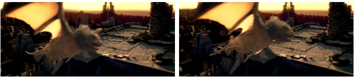
(a) Image att−1 (b) Image att _(c) Image att+ 1

Figure 2.3: A situation where multi-frame optical flow is essential. The

dragon’s wing in the frame at time t goes out of frame at time t+ 1,

mak-ing it nearly impossible to recover its motion of usmak-ing two-frame optical flow.

The wing, however, is visible in frame t−1, which provides information about

its motion.

2.6 Multi-frame optical flow

Optical flow is often posed as a two-frame problem: estimate the apparent motion

from the frame at timetto timet+1. While this works for simple situations, there

is sometimes insufficient information in only two frames for a good correspondence

to be found. An example of this situation is shown in Figure 2.3. In this figure,

the dragon’s wing at timetis no longer visible at timet+1, and thus no amount of

smoothness constraint could propagate flow to this occluded region since the entire

region is occluded. However, in the previous frame at timet−1 the dragon’s wing is still visible and this provides information about the motion of the wing. The

use of more than two frames in optical flow can thereby provide useful information

and improve results.

Despite the relative lack of modern multi-frame optical flow algorithms, attempts

have been made to model temporal consistency back to the work of (Murray and

Buxton,1987). The most common idea is to impose a sort of temporal regularity

similar to the spatial regularity term. In particular, it is assumed that the flow

estimates are smooth over time. In (Nagel, 1990), Nagel extended the idea of

(47)

A related flow-driven temporal smoothness constraint was proposed subsequently

in (Weickert and Schnörr, 2001).

However, in contrast to the spatial term where pixels can be connected with a

static set of neighbors in a grid, a temporal continuity constraint works better if

it is paired with the pixel that it matches to in the subsequent image. A primary reason why simply enforcing smoothness across the same pixel location over time

does not work well is that many image sequences have a low frame-rate relative

to their motions and thus temporal derivatives are meaningless. Of course, this

pixel correspondence is not known beforehand, leading to a difficult optimization

problem. In (Black and Anandan, 1990), the motion of a pixel was compared

with an average of the same track point’s previous velocities. In (Salgado and

Sánchez,2007), a model is used that penalizes deviations between velocity vectors

in subsequent frames for matched pixels. A novel parameterization of temporal

smoothness was presented in (Volz et al., 2011), where a constraint was imposed

by parameterizing all flow values with respect to a center frame. In this model,

five frames are used for motion estimation. Rather than having a separate flow

estimate between all successive pairs of frames and needing to track points over

time, the flow values are estimated as an offset such that flow from the center frame to any other frame can be obtained by summing the flow estimates at the

same pixel location. This allows for temporal constraints to be naturally placed

along the temporal dimension.

Temporal consistency has also been enforced in layered models. In (Sun et al.,

2010b, 2012), a term of the cost function encourages pixels connected based on

the current flow estimate to have similar layer assignments.

(48)

stereo. In multi-view stereo, more than two images are used for reconstruction and

the result is a 3D surface of the imaged scene. In this case, a single point on the

object is seen from multiple images. In (Newcombe et al., 2011), the data costs

from multiple images are averaged, while in our method we take the minimum

of several data costs to allow for occlusions. A similar approach was also taken

in (Szeliski and Coughlan, 1997) and (Okutomi and Kanade, 1993). In (Szeliski

and Coughlan, 1997; Sun et al., 2000) in particular, linear flow was assumed for

multi-frame flow estimation. In (Kang et al.,2001), multiple frames were handled

within a stereo correspondence problem by selecting a subset of frames for each

pixel that were likely to be unoccluded.

In Chapter 4, we present a novel method of incorporating temporal information

into any optical flow algorithm with minimal complexity, leading to very

high-quality flow estimates on difficult image sequences.

2.7 Fusion methods

Fusion methods are an interesting optical flow technique, where multiple estimates

of optical flow are combined in order to improve results. Most often, this is done

by using multiple algorithms or parameter values to estimate the same two-frame

motion. In (Lempitsky et al., 2008), flow estimates were generated using the

Horn-Schunck and Lucas-Kanade algorithms with various parameter settings. The

objective of the fusion step in (Lempitsky et al.,2008) was to directly minimize the

energy of a global MRF model. This was done by considering two flow estimates

at a time and performing optimization using a discrete move-making algorithm

(Boykov et al., 2001). In (Jung et al., 2008), multiple local minima of an MRF

(49)

(a) 4-connected neighborhood

(b)

8-connected neighborhood

Figure 2.4: 4- and 8-connected MRF neighborhoods. A 4-grid is more

com-monly used due to its simplicity.

related method in (Chen et al.,2013) produced a set of proposal motion models and

then assigned each pixel to the models using an energy minimization framework.

Fusion can also be cast within a classification framework. In (Mac Aodha et al.,

2013), a random forest classifier was trained to estimate how accurate the optical

flow estimate is at each pixel. This confidence could potentially be used to combine

several algorithms based on which is more confident. A similar approach was

taken in (Mac Aodha et al.,2010), where a classifier was used to determine which

algorithm from a set of them would likely give the most accurate solution at each

pixel. In Chapter4, we show how a related fusion method can be used to not only

fuse multiple algorithms, but also to fuse temporal information that we call the

inertial estimates of optical flow.

2.8 Discrete optimization

In the methods discussed so far, optical flow has been treated as a continuous

optimization problem, where the offset assigned to each pixel location is potentially

Discrete and Continuous Optimization for Motion Estimation