DESIGN FLOOD ESTIMATION FOR
UPPER KRISHNA BASIN THROUGH
RFFA
AKSHAY R. THORVAT1
1
Assistant Professor, Department of Civil Engineering, KIT’s College of Engineering, Kolhapur, 416234,
Maharashtra, India. [email protected]
MANOJ M. MUJUMDAR2
2
Professor, Department of Civil Engineering, KIT’s College of Engineering, Kolhapur, 416234,
Maharashtra, India. [email protected]
Abstract:
The objective of this study is to establish a regional relationship between mean annual peak flood and the catchments area based on the frequency analysis for available annual peak flood for various gauging sites of hydro logically homogeneous region of Krishna basin, and to use the same for estimating the floods for various recurrence intervals for the catchments which are not used for analysis. This paper describes a study carried out for the Krishna basin with annual peak flood series data available for 24 sites for varying number of years. The Index flood method was used for analysis. Out of 24 sites, 4 sites were omitted after the USGS homogeneity test since they fall outside the envelope curves of homogeneity test. From the remaining 20 sites only 18 sites were considered for the analysis and data of other 2 sites were used as test sites for judging the performance of the developed regional formulae.
Keywords: Design flood; Index flood method; Homogeneity test; ungauged sites.
1. Introduction
Flood estimates are required for the design and economic appraisal of a variety of engineering works, including dam, spillways, bridges and flood protection works. Flood estimates are also required for the safe operation of flood control structures, for taking emergency measures such as maintenance of flood levees, evacuating the people to safe localities etc. Two main approaches are available for flood estimation viz., deterministic approach and statistical approach. Deterministic approach assumes that input, say, the precipitation is related to the output in a predefined manner and there is no uncertainty involved in arriving at the output, say the discharge., whereas the statistical approach treats the inter-relationship between processes as governed by theory of statistics. The inter-relationship between processes is established through the measures of correlation, the processes considered may be multivariate or, univariate. For example, the rainfall-runoff process may be considered as multivariate while, the consideration of maximum annual peak series falls under univariate process. Flood frequency analysis deals with univariate process comprising of maximum peak flow values. Before discussing the frequency analysis it is necessary to distinguish between the terminologies of prediction and forecasting from the consideration of their field use.
rainfall-2. Elements of Flood Frequency Analysis
The problem of flood frequency prediction i.e. Estimation of the relationship between the magnitude of peak flow and us corresponding return period is a central one in the field of applied hydrology. Attempts to solve this problem are usually based on (a) the analysis of a record of peak flow data at the site in question and (b) use of previously established relationship between the characteristics of other catchments in the region and the parametric values of the corresponding magnitude return period relationship. The latter approach is known as regional frequency analysis used for estimating floods at sites where there is a very short peak flow record or no record available.
2.1. Basic Assumptions in Flood Frequency Analysis
Three assumptions are fundamental to the flood frequency analysis
2.1.1. Sample is Representative of Population:
Hydrologic data are mostly available as samples of limited sizes. Using statistical principles we extract the needed information from the available sample data and conclude about the characteristics of the population. Since any survey or any attempt cannot exhaust all possible events of a variable, we assume that the sample is representative of population.
2.1.2. Independence of Peak Flows:
We assume that that the sample of peak flows available is independent of each other and they are assumed to be evolved from a purely random process.
2.1.3. Homogeneity of Peak Flows:
When a series of events arranged in time show no systematic variations in time (e.g., a seasonal variation or an increasing or diminishing trend) so that we may say that the probability of an event in a period (t) is independent of the location, the series is said to be homogeneous The factors which affect the homogeneity of peak flows are the development in the catchments over time such as deforestation, urbanization, flood control works, earthquakes etc.
2.2. Regional Flood Frequency Analysis
There have been significant developments and studies in the area of regional flood frequency analysis in India as well as abroad. Estimation of regional flood frequency parameters is performed for a specific site for two reasons:
• Because of the sample variations present in the short hydrologic records, frequency estimates of rare events based on at site frequency analysis are subjected to large error and thus unreliable. This error can be reduced by combining data from many more sites,
• There are many more sites in the same region where hydrologic data are not available but design flood estimates are needed for the design of small structures. In such a situation regional flood frequency analysis helps in transferring the knowledge arrived from gauged sites to ungauged sites.
2.3. Importance of Statistical Analysis in Hydrology
The random variability of such hydrologic variables as stream flow and precipitation has been recognized for centuries. The general field of hydrology was one of the first areas of science and engineering to use statistical concepts in an effort to analyze natural phenomena. The use of statistics in hydrology provides the information about various parameters and distribution of random variables of importance to design and operation of structures. These parameters and distributions are estimated as approximations from the available data because they cannot be determined exactly.
2.3.1. Probability Distributions Used in Hydrology:
One of the major problems faced in hydrology is the estimation of design flood from fairly short data. If the length of data is more, then the same data can be used to estimate design flood, but the length of data generally available is very less. So the sample data is used to lit frequency distribution which in turn is used to extrapolate from recorded events to design events either graphically or by estimating the parameters of frequency distribution.
Graphical method is having the advantage of simplicity and visual presentation. But the main disadvantage is that different engineers will fit different curves.
The following continuous distributions are used to fit the annual peak discharge series.
• Normal distribution
• Log normal distribution
• Pearson type III distribution
• Exponential distribution
• Gamma distribution with two parameters
• Log Pearson type III distribution
• Extreme value distributions
2.4. Flood Frequency Analysis
Flood frequency analysis is a tool being widely used for predicting the future flood at different recurrence intervals. The reliable estimates of the magnitude and frequency of occurrence of flood are essential to the proper design of hydraulic structure across a river as well as to identify the flood risk area. Mainly there are two methods of estimating the floods; i.e., deterministic and statistical approach. In the deterministic approach, the rainfall-runoff relationships established based on the physical concepts of the various hydrological processes are used to estimated the floods. In the statistical approach, the past records of flood peaks are subjected to the statistical analysis which provides the distribution pattern for the flood peaks. The frequency analysis is a statistical technique by means of which it is possible to estimate the floods of various magnitudes and their frequencies. The flood frequency analysis for a river site with a long record can be based almost exclusively on the flood record at that site.
3. Data Requirement
All frequency techniques are totally data dependent. An assumption must be made of a theoretical frequency distribution suitable for the population events and the statistical parameters of the distribution must be computed from the sample data. Two types of sample data, namely (i) annual peak flood series and (ii) partial duration series may be used for flood frequency analysis.
Annual peak flood series is arrived at from the recorded flood peaks by picking up only one event from each year of the record. Annual peak flood series ensures complete randomness of the data and thus assumption of randomness is satisfied. But a disadvantage of using this series for analysis is that the second or third highest events in a particular year may be higher than some of the year's annual peak floods and still they are totally disregarded in the analysis. Such a disadvantage is remedied by using the partial duration series in which all the events above a certain threshold are included in the analysis. However care should be taken not to include those peaks which are dependent as the assumption of randomness would be violated. This can be achieved by ensuring that consecutive flood peaks are separated by a recession of a suitable length of time. The procedures for dealing with dependent data are still in research stage.
As a preliminary step the basic data should be screened and adjusted to remove, as far as possible, any non-conformity that may exist. The following are the more important considerations (CWC, 1969).
• Effect of man made changes in the regime of flow should be investigated and adjustment be made as required.
• Changes in the stage discharge relation render stage records non homogeneous and unsuitable for frequency analysis studies. It is therefore preferable to work with discharges and if stage frequencies are required, refer the results to the most recent rating.
• Any useful information contained in data publications and manuscripts should be made use of after proper scrutiny.
The records used for the frequency analysis should satisfy certain assumptions in order to have meaningful estimates;
• Data should be random
• Data considered for analysis should be homogeneous
• Data should be of good quality
• Data should be representative of the population
• Sample of data should be long enough to provide reliable estimates of the parameters.
4. Description of Study Area
The Krishna basin for which sufficient annual peak flood series at number of gauging station were available was selected as the study area. The total catchments area of the basin considered for the analysis is 90,000 sq.km and is located between longitude of 73°E to 72°E and latitude of 15°N to 19°N and it comprises the part of Maharashtra and Karnataka states. The figure 1 shows the river system and gauging stations with all its tributary of river Krishna. The drainage area of these gauging sites varies from 540 sq.km to 70,000 sq.km. The main tributaries of river Krishna are river Bhima, Ghataprabha, Malaprabha and Bhadra. The Tunga-Bhadra basin which forms a part of the Krishna basin has not been included in the study.
5. Methodology
The method used in the present study to carry out the regional flood frequency analysis involves the USGS method. The USGS method for estimating the floods of given recurrence intervals for ungauged catchments consists of following sequential steps:
• Select gauged catchments within region having more or less similar hydrological characteristics to that of the ungauged catchments.
• Establish flood frequency curves for each gauging station using EV-I distribution probability paper.
• Estimate mean annual flood Q2.33 at each gauging station.
• Test the homogeneity for gauged catchments.
• Rank ratios of selected return period floods to the mean annual flood at each station, and
• Compute median flood ratio for each of the selected return period of step (5), multiply by the estimated mean annual flood of the ungauged catchment’s and plot them against recurrence interval on Gumble probability paper.
Fig. 1. Location Map of Study Area Showing CWC Drainage Basins and River Network
6. Results and Discussions
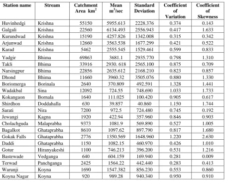
Table 1. Preliminary Statistics
Station name Stream Catchment Area km2
Mean m3/sec
Standard Deviation
Coefficient of Variation
Coefficient of Skewness
Huvinhedgi Krishna 55150 5955.613 2228.376 0.374 0.143
Galgali Krishna 22560 6134.493 2556.943 0.417 1.633
Kurundwad Krishna 15190 4257.826 1342.008 0.315 0.342
Arjunwad Krishna 12660 3563.538 1677.299 0.421 0.522
Karad Krishna 5462 2555.545 1529.461 0.599 0.833
Yadgir Bhima 69863 3681.1 2935.770 0.798 1.310
Takli Bhima 33916 2930. 618 2565.100 0.875 0.709
Narsingpur Bhima 22856 2635.612 2168.210 0.823 0.857
Dhond Bhima 11660 3960.32 3505.076 0.880 1.330
Boriomerga Borinala 2640 370.809 492.591 1.328 1.441
Wadakbal Sina 12092 724.55 748.690 1.033 1.733
Kokangaon Bornala 1640 111.025 100.420 0.905 0.617
Shirdhon Doddahalla 630 39.857 40.860 1.150 1.744
Sarati Nira 7200 972.5 724.480 0.745 0.192
Jewangi Kagna 1920 422.94 357.960 0.846 0.903
Cholachguda Malaprabha 9373 1081.9 569.890 0.527 1.005
Bagalkot Ghataprabha 8610 1097.62 897.790 0.817 1.680
Gokak Falls Ghataprabha 2776 1350.569 1648.960 1.220 2.630
Daddi Ghataprabha 1150 1082.15 460.970 0.426 1.010
Gotur Hiranyakeshi 1100 746.213 396.200 0.531 1.216
Bastewade Vedganga 640 604.159 169.940 0.281 0.009
Terwad Panchganga 2425 1564.22 442.440 0.283 0.413
Warunji Koyna 1690 1547.382 856.230 0.553 0.860
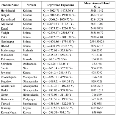
Table 2. Regression Equations and Mean Annual Flood
Station Name Stream Regression Equations Mean Annual Flood Q2.33
Huvinhedgi Krishna QT = 5023.71+1675.76 YT 5928.1642
Galgali Krishna QT = 5042.48+ 1980.34 YT 4662.3043
Kurundwad Krishna QT =3668.5+ 1059.75 YT 4284.5058
Arjunwad Krishna QT =2834.2 + 1311.51 YT 3623.1202
Karad Krishna QT =1873.12 + 1226.31 YT 2498.9459
Yadgir Bhima QT =2399.47+ 2304.57 YT 3551.0472
Takli Bhima QT =1812.07 + 2011.38 YT 2830.4004
Narsingpur Bhima QT =1670.86 + 1734.83 YT 2554.53028
Dhond Bhima QT =2470.79+ 2678.5 YT 3824.6316 Boriomerga Borinala QT =172.91 + 355.86 YT 360.2595
Wadakbal Sina QT =415.45 + 555.83 YT 701.8341
Kokangaon Bornala QT =66.6 + 79.3 YT 106.9816
Shirdhon Doddahalla QT =21.25 + 33.45 YT 38.6768
Sarati Nira QT =665.14 + 552.72 YT 936.8976 Jewangi Kagna QT =264.2 + 285.45 YT 408.3792 Cholachguda Malaprabha QT =826.12 + 459.94 YT 1047.581
Bagalkot Ghataprabha QT =1093.21 + 994.24 YT 839.9728
Gokak Falls Ghataprabha QT =737.36 + 1102.68 YT 1308.2718
Daddi Ghataprabha QT =882.85 + 358.39 YT 1037.1612
Gotur Hiranyakeshi QT =573.04 + 311.40 YT 716.569
Bastewade Vedganga QT =537.58 + 119.72 YT 577.1416
Terwad Panchganga QT =1384.96 + 322.368 YT 585.058
Warunji Koyna QT =1172.27+ 674.53 YT 1489.8756
Koyna Nagar Koyna QT =598.33+ 703.0 YT 959.089
Table 3. Calculation for Absolute Error for Test Site Takali
Index Flood Method
Regional FF Curve QT/Q2.33 =0.6970 + 0.5220 YT
Takali QT =1812.07 + 2011.38 YT
Sr No. Return Period
Estimated Actual Parameter
Estimated Regression Parameter
Absolute Difference Absolute Error Site-1 Site-2 Site-1 Site-2
1 5 4829.019 4223.577 605.442 420.681 0.125 0.087
2 10 6338.414 5341.487 996.926 763.262 0.157 0.120
3 20 7786.261 6413.814 1372.447 1091.873 0.176 0.140
4 50 9660.351 7801.831 1858.521 1517.228 0.192 0.157
5 100 11064.718 8841.954 2222.764 1835.971 0.201 0.166
6 200 12463.961 9878.282 2585.679 2153.551 0.207 0.173
7 500 14309.995 11245.520 3064.475 2572.537 0.214 0.180.
Sum 1.2738 1.0233
Table 4. Calculation for Absolute Error for Test Site Gotur
Index Flood Method
Regional FF Curve QT/Q2.33 =0.6970 + 0.5220 YT
Gotur QT =573.04 + 311.40 YT
Sr No. Return Period
Estimated Actual Parameter
Estimated Regression Parameter
Absolute Difference Absolute Error Site-1 Site-2 Site-1 Site-2
1 5 1040.121 751.043 289.078 75.260 0.278 0.072
2 10 1273.804 949.832 323.972 136.800 0.254 0.107
3 20 1497.959 1140.515 357.444 195.830 0.239 0.131
4 50 1788.104 1387.334 400.769 272.239 0.224 0.152
5 100 2005.526 1572.291 433.236 329.497 0.216 0.164
6 200 2222.156 1756.572 465.584 386.497 0.210 0.174
7 500 2507.957 1999.697 508.260 461.811 0.203 0.184
Sum 1.623 0.985
Average 0.2312 0.1410
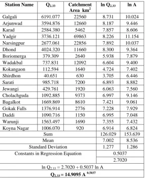
Table 5. Calculation for Relationship between Q2.33 and Catchment Area
Station Name Q2.33 Catchment
Area km2
ln Q2.33 ln A
Galgali 6191.077 22560 8.731 10.024
Arjunwad 3594.876 12660 8.187 9.446
Karad 2584.380 5462 7.857 8.606
Yadgir 3736.121 69863 8.226 11.154
Narsingpur 2677.061 22856 7.892 10.037
Dhond 4024.320 11660 8.300 9.364
Boriomerga 379.309 2640 5.938 7.879
Wadakbal 737.831 12092 6.604 9.400
Kokangaon 112.594 1640 4.724 7.402
Shirdhon 40.651 630 3.705 6.446
Sarati 985.718 7200 6.893 8.882
Jewangi 429.761 1920 6.063 7.560
Cholachguda 1092.885 9373 6.997 9.146
Bagalkot 1669.869 8610 7.421 9.061
Gokak Falls 1376.914 2776 7.228 7.929
Daddi 1090.716 1150 6.995 7.048
Warunji 1563.497 1690 7.355 7.432
Koyna Nagar 1006.070 920 6.914 6.824
Sum 126.029 153.639
Mean 7.002 8.536
Standard Deviation 1.277 1.286
Constants in Regression Equation 0.5037 2.7020 ln Q2.33 = 2.7020 + 0.5037 ln A
7. Conclusion
• Four sites namely Huvinhedgi, Kurundwad, Bastewade and Terwad are not in homogeneity area.
• The Regional Flood Frequency curve for upper Krishna Basin is:
QT/Q2.33= 0.6970+ 0.5220 YT
• The relationship between Q2.33 and the area for upper Krishna basin is:
Q2.33= 14.9095.A0.5037
• The absolute errors in flood prediction using atsite parameter & atsite mean are 14.10 % and 14.60 % for Gotur and Takali respectively.
• The absolute errors in flood prediction using regional parameter and regional mean are 23.12 % and 18.19 % for Gotur and Takali respectively.
• Further research is necessary to improve regional mean values. The regional mean value largely depends on catchment area. However Q2.33 dependent on other catchment characteristics such as drainage density, average elevation of catchment, average slope of stream and catchment, average annual rainfall, land use and land cover etc. should be tried for further improvements.
8. References
[1] B. N. S. Chalam, M. Krishnaveni, M. Karmegam (1996), “Correlation Analysis of Runoff with Geomorphic Parameters”, Journal of Applied Hydrology, Vol. IX, No.3, 4 1996, 24-31.
[2] Burn, D.H. (1990), “Evaluation of regional flood frequency analysis with a region of influence approach”, Water Resour. Res.”, 26(10), 2257 – 2265.
[3] Central Water and Power Commission (1969), ‘Estimation of Design Flood-Recommended Procedure’. [4] Cunnane, C. (1988), “Methods and merits of regional flood frequency analysis.” J. Hydrol., 100, 269 – 290.
[5] Dalrymple T. (1960), “Flood frequency methods”, U. S. Geol. Surv. Water supply pap, 1543A, U.S. Govt. Printing office, Washington, D.C., 11 – 51.
[6] G. Bhaskaran, R. Jayakumar, J. Moses Edwin, K. Kumaraswamy, “Identification of Influential Geomorphic Parameters in Hydrological Modelling through Numerical Analysis”, Journal of Applied Hydrology, Vol. XV, No. 1, 1-8.
[7] Hosking, J.R.M, Wallis, J.R. (1990), Regional Flood Frequency Analysis, IBM Research Report.
[8] Hosking, J.R.M, Wallis, J.R. (1993), “Some statistics useful in regional frequency analysis” Water Resour. Res., 29(2), 271 -281 [9] Lim, Y.H., Lye, L.M. (2003), “Regional flood estimation for ungauged basins in Sarwak, Malaysia”, Hydrological Sci. J., 48 (1),
79-93
[10] National Institute of Hydrology, Roorkee, “Flood Frequency Analysis” Lecture notes.
[11] Seth, S.M., Kumar, R., Singh, R.D. (1995), “Development of regional flood formula for Mahanadi sub zone, 3(d)” NIH Technical Report, TR (BR )- 134.