Applying Computational Intelligence Techniques to QoS Time Series Forecasting in Services Computing

Applying Computational Intelligence Techniques to QoS

Time Series Forecasting in Services Computing

Yang Syu

_{, Yong-Yi FanJiang}

1_{Institute of Information Science, Academia Sinica, Taipei City, Taiwan.}

2_{Department of Computer Science and Information Engineering, Fu Jen Catholic University, New Taipei City,}

Taiwan

* Corresponding author. Email: [email protected] Manuscript submitted May 10, 2018; accepted July 8, 2018. doi: 10.17706/jcp.13.9.1010-1026

Abstract: Recently, the forecasting of dynamic Quality of Service (QoS) values for Web Services (WSs) has become an emerging topic in services computing. In most previous research, various time series forecasting methods have been used to address this problem. In this paper, we propose the use of two computational intelligence techniques, namely, genetic programming (GP) and support vector regression (SVR). To demonstrate the forecasting performance of the two proposed techniques, we compare them with the conventional methods based on experiments run on a real-world dynamic QoS time series dataset. Our experimental results show that the proposed GP and SVR methods outperform the conventional methods in both training (in-sample) and testing (out-of-sample) accuracy. Between the two proposed approaches, we find that GP might be the better choice overall. In terms of training performance, GP is superior in terms of both the individual and average experimental results; however, this is not the case for testing performance. In terms of testing accuracy, SVR outperforms GP in many individual experiments; however, SVR also yields extremely poor forecasting accuracy in several individual experiments, indicating that it is unstable and unreliable. In many of the individual experiments, GP is only insignificantly inferior to SVR, and it still achieves the best average forecasting accuracy according to two of the three considered measures.

Key words: Time series forecasting, quality of service, computational intelligence techniques, support vector regression, genetic programming.

1.

Introduction

The QoS attributes of a Web Services (WS) can be broadly divided into two categories, namely, static QoS attributes and dynamic QoS attributes. The former are QoS attributes with fixed values (e.g., price), whereas the latter are attributes whose values vary over time (e.g., response time and availability). Dynamic QoS attributes are the focus of this study. The real examples of the variations in the dynamic QoS attributes of WSs (dynamic QoS time series) can be found in Section II of [1], Section 3.2 of [2], Section 2 of [3], Section 3.3 of [4], Section 8 of [5], and Section III.B of [6].

review and discuss in Section 2.

To address the problem of predicting dynamic QoS values, as shown in Section 2 of this paper, most previous research has treated the problem as one of time series forecasting, and various statistics-based methods for time series forecasting have been employed, such as Auto-Regressive Integrated Moving Average (ARIMA) models and Exponential Smoothing (ES) methods. In this paper, instead of using traditional time series forecasting methods, we propose to address the problem using computational intelligence techniques, such as genetic programming (GP) and support vector regression (SVR). More specifically, we use GP and SVR to seek a predictor that can produce accurate dynamic QoS predictions.

The manner in which prediction is performed using the adopted computational intelligence techniques (i.e., the form of the predictor and the way in which it is generated) differs from the approach used in traditional time series methods; indeed, computational intelligence techniques are quite innovative compared with traditional time series methods, which have a long history of development based on statistical techniques. The hope is to take advantage of their unique features and advantages (which are explained in detail in Section 4 of this paper) to achieve better forecasting performance (i.e., lower forecasting error and higher prediction accuracy). Another motivation for investigating the use of computational intelligence techniques for this purpose is that they have been successfully applied for time series forecasting in other application domains; for example, GP has been applied to financial time series in [8]-[11] and for supply chain management in [12].

In this study, we also consider several conventional methods for comparison, including the two current de facto solutions for time series forecasting, i.e., ARIMA models and ES methods [13]. Before we describe the proposed computational intelligence techniques and the conventional methods with which they are to be compared, the problem to be solved and the accuracy metrics to be used are formally defined. Finally, for the evaluation of the considered approaches in a realistic scenario, we present a set of experiments run on a real-world dynamic QoS dataset and then analyze and discuss the experimental results in detail.

Below, we describe the contributions of this paper. First, to the best of our knowledge, we are the first to propose the application of these two computation intelligence techniques, i.e., GP and SVR, to solve the dynamic QoS forecasting problem. Based on our experimental results, we find that overall, the two proposed techniques outperform the traditional, well-developed time series methods in both training and testing forecasting accuracy. Second, because we include most representative time series approaches in our comparison, this study can serve as a guide for WS consumers when they wish to choose or develop a dynamic QoS forecasting solution for their own purposes. Finally, this paper comprehensively documents our study. All elements of the study, including the problem to be solved, the methods used to evaluate forecasting accuracy, and the proposed and conventional solutions are formally described and defined. Such definitions are partially or completely lacking in most existing works. However, without a formal mathematical definition of the considered problem, for example, many specifics remain unknown, thereby preventing further evaluations using the same problem specifications.

considered measures of forecasting accuracy.

The remainder of this paper is organized as follows. Section 2 reviews existing studies on dynamic QoS time series forecasting. The forecasting problem to be solved and the accuracy measures used in this paper are defined in Section 3. Subsequently, Section 4 and 5 introduce the proposed computational intelligence techniques and the conventional methods considered for comparison, respectively. Our experimental environment and results are fully described in Section 6, and the results are analyzed and discussed in detail in Section 7. Finally, Section 8 concludes the paper.

2.

Related Work

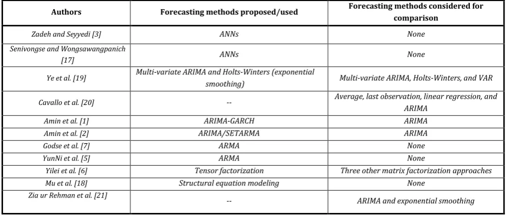
This section reviews the existing research on dynamic QoS time series forecasting. Table 1 presents the reviewed studies; each study is described in the table in terms of its proposed forecasting approach and the methods considered for comparison. From Table 1, it is clear that most previous works have used various traditional time series methods to approach the problem, mostly ARIMA and ES methods, because it is intuitive to adopt such well-developed, fully elaborated methods based on traditional disciplines (in this case, statistics and time series forecasting) to address the problem of interest.

However, there are also a few works, i.e., [3] and [17], that have employed artificial neural networks (ANNs), another common computational intelligence (or machine learning) technique. Although the authors of [3] claimed that ANNs, with their flexibility and strong analysis capability, represent the strongest competition for traditional time series methods in solving the dynamic QoS time series forecasting problem, our experimental results indicate that ANNs are not as accurate as GP or SVR. The table also lists two exceptional cases in which neither conventional time series methods nor computational intelligence techniques were used, namely, [6] and [18]. The former addressed a three-dimensional QoS forecasting problem, which is not exactly identical to the problem targeted in this study, and the latter used structural equation modeling, which is rarely employed in time series forecasting.

In this paper, most of the time series methods presented in Table 1 are considered as methods for comparison; thus, their technical details can be found in Section 4 (ANNs) and Section 5.

Table 1. A List of Existing Dynamic QoS Time Series Forecasting Approaches and the Methods with which They have been Compared

Authors Forecasting methods proposed/used Forecasting methods considered for comparison

Zadeh and Seyyedi [3] ANNs None

Senivongse and Wongsawangpanich

[17] ANNs None

Ye et al. [19] Multi-variate ARIMA and Holts-Winters (exponential

smoothing) Multi-variate ARIMA, Holts-Winters, and VAR

Cavallo et al. [20] -- Average, last observation, linear regression, and ARIMA

Amin et al. [1] ARIMA-GARCH ARIMA

Amin et al. [2] ARIMA/SETARMA ARIMA

Godse et al. [7] ARMA None

YunNi et al. [5] ARMA None

Yilei et al. [6] Tensor factorization Three other matrix factorization approaches

Mu et al. [18] Structural equation modeling None

Zia ur Rehman et al. [21]

-- ARIMA and exponential smoothing

This section formally defines both the forecasting problem to be addressed and the accuracy measures to be used for performance evaluation.

3.1.

Formal Problem Definition

Before formulating the problem, we first define the dynamic QoS time series of interest. In this paper, we consider the response time of a WS as our forecasting target because it has been widely used in many previous studies.

A dynamic QoS time series (TS) is defined as

QoS1…l = {q1, q2, …, ql-1, ql},

wherelis the length of the TS, i.e., the number of (response time) observations it contains; QoS1…l denotes

the set of WS response time observations recorded during the period 1, …, l; and qi represents the response

time of the WS at time i. Furthermore, a TS can be split into two segments for analysis, namely, a training sub-TS TraQoS1…tral and a testing sub-TS TesQoS1…tesl:

QoS 1…l = {TraQoS 1…tral , TesQoS 1…tesl}

and

TraQoS1…tral = {tra_q1, tra_q2, …, tra_qtral-1, tra_qtral},

TesQoS1…tesl = {tes_q1, tes_q2, …, tes_qtesl-1, tes_qtesl},

where tral and tesl are the lengths of the training sub-TS and the testing sub-TS, respectively, and tral +

tesl = l. Note that tra_q1 = q1 and tes_qtesl = ql and that tra_qtral = qtral and tes_q1 = qtral+1. The training

sub-TS is used to generate a predictor and to calculate the training (in-sample) accuracy, and the corresponding testing sub-TS is used to measure the testing (out-of-sample) forecasting accuracy.

To generate a set of QoS forecasts, a forecasting approach must consist of two phases, i.e., predictor generation and forecast generation. Predictor generation can be simply expressed as follows:

QoSPredictor ← FA(TraQoS1…tral),

where QoSPredictor denotes the QoS (response time) predictor generated by forecasting approach FA with

TraQoS1…tral as the available training data (i.e., the input to the algorithm). The forecasting approaches

proposed in this study and the conventional approaches against which they are compared (namely, the various FA) are introduced in Section 4 and Section 5, respectively.

After a predictor is obtained, the algorithm proceeds to forecast generation. In this study, we consider one-step-ahead forecasting (a common assumption in current research); thus, to obtain a set of forecasts, the predictor must be iteratively applied to a set of predictor inputs that is constantly being updated. For example, the process of obtaining a set of QoS forecast values (FTesQoS1…tesl) is expressed as follows:

ftes_q1 ← QoSPredictor(TraQoS1…tral),

ftes_q2 ← QoSPredictor(TraQoS1…tral, TesQoS1),

…..

ftes_qtesl ← QoSPredictor(TraQoS1…tral, TesQoS1…tesl-1),

and

FTesQoS1…tesl = {ftes_q1, ftes_q2, …, ftes_qtesl}.

Consequently, FTesQoS1…tesl can be used to calculate the testing forecasting accuracy, as shown in the next

section. Similarly, a set of training forecasts, FTraQoS1…tral, can be obtained in the same way for the

calculation of the training accuracy.

3.2.

Measures of Forecasting Accuracy

In this paper, both training (in-sample) accuracy and testing (out-of-sample) accuracy are considered. For both of them, the mean absolute errors (MAEs) and mean absolute percentage errors (MAPEs) of each forecasting approach are evaluated. In addition, for testing accuracy, we also consider the mean absolute scaled errors (MASEs) because the MASE is the recommended standard evaluation measure for time series forecasting, especially when the results of multiple forecasting problems are to be integrated (across multiple time series of different scales) [14], [15].

The MAE of a testing forecasting result is calculated as follows:

.

The MAE is the most common and basic measure in time series forecasting. It is simple and intuitive, directly representing an average error value. However, the MAE is a scale-dependent measure; given only an MAE value, it is difficult to determine the real level of forecasting error that value represents. To overcome this shortcoming of the MAE, the MAPE was defined as shown below:

.

MAPE values are percentages; therefore, the MAPE represents the relative degree of forecasting error (compared with the actual observed value tes_qi). The MAPE is a scale-independent measure; thus, it can be

used to compare forecasting performance across disparate datasets. However, the MAPE still has some disadvantages, such as the fact that its value is infinite or undefined if tes_qi = 0 for any i during the

considered period; thus, the scale-free MASE measure was proposed by the authors of [14], [15] to avoid the disadvantages of the MAE and MAPE.

The MASE for a set of testing forecasts is calculated as follows:

.

The MASE is similar to the MAPE; the main difference between them is that the MASE is calculated by using the training (in-sample) MAE value obtained via the naïve approach (introduced in Section 5) as the denominator in place of the actual observed value tes_qi that is used to calculate the MAPE.

Regarding the training MAE and MAPE measures, they can be calculated in the same way as the testing MAE and MAPE measures, respectively, with the only difference being that the inputs to these measures are

TraQoS1…tral and FTraQoS1…tral.

4.

Computational Intelligence Techniques

4.1.

Genetic Programming (GP)

GP is a variant of the genetic algorithm (GA) approach, and both techniques follow a similar problem-solving (evolution) process. However, they differ in the nature of the elements (solutions) that are sought and operated on during that evolution process. GAs evolve and search for a direct answer to the problem of interest (e.g., a set of values for a parameter optimization problem); by contrast, GP looks for a solver (in this paper, a dynamic QoS predictor, i.e., QoSPredictor as defined in Section 3.1) that can provide an answer for a given problem instance.

GP differs from the other approaches considered in this study in that it does not assume any specific form of the solver (predictor) that is sought and thus is not restricted by any default assumptions regarding the construction of the solver/predictor during its evolution process. In fact, based on the defined function set (the set of allowed expression operators) and terminal set (the set of allowed operands), GP searches for optimal solvers within the space consisting of all valid expression combinations (solvers). For example, suppose that the function and terminal sets are {+, -, *, /} and {1~10, qcur, qcur-1, qcur-2}, respectively, where

cur represents the present, the one-step-ahead forecasting target is qcur+1 (the prediction thereof is

represented by fcur+1), and qcur, qcur-1, and qcur-2are the lagged values (i.e., the available past observations);

then, all valid expression combinations consisting of the operators and operands that appear in these sets, such as fcur+1 = ((3qcur-1/4.32) – (qcur + qcur-2)*3.12), which is impossible to consider in other forecasting approaches, are contained in the explored search space. By contrast, as presented in the following sections, each of the other forecasting approaches employs a certain expression (predictor) skeleton; consequently, the only elements that can be modified are the parameters of that skeleton, thereby placing a considerable restriction on the expressions/predictors that can be considered. Theoretically, with GP, all possible valid predictor/expression combinations are covered (contained in the search space), and thus, this approach is more powerful and complete than any other forecasting approach because for the other approaches, the search space is limited by the default predictor/expression skeleton; the optimal solver could possess an unusual or complicated expression structure lying just outside the search space, in which case it would not be found.

Furthermore, instead of performing a complete, brute-force search in an enormous space whose size is determined by the numbers of operators and operands in the corresponding function and terminal sets, the GP algorithm executes a heuristic search driven by its fitness function and three bio-inspired GP operators, i.e., selection, crossover, and mutation (the last two operators are each associated with a probability for determining whether the corresponding operation is to be executed in each possible instance). We present a succinct, pseudocode-like description of GP below.

1. Initialize randomly CurPopulation (the first generation); 2. while stopping condition is not satisfied

3. Evaluate each Solver in CurPopulation using fitness function;

4. Generate a new empty population NewPopulation;

5. whileNewPopulation is not full

6. Select two Parents from CurPopulation based on fitness value;

7. CrossoverParents according to crossover probability;

8. Mutate first Parent according to mutation probability;

9. Mutate second Parent according to mutation probability;

10. Push Parents into NewPopulation;

11. CurPopulation ← NewPopulation;

12. Return best solver in CurPopulation;

once the last generation has been produced, the algorithm returns the solver with the best survivability (represented by its fitness value) in the population as the answer (solver) for the problem of interest. The evolution of the solvers in the population is driven by the four components of the GP algorithm, namely, the fitness function and its three operators. The core of the GP algorithm is the designed fitness function, which must accurately evaluate each solver and assign it a score (fitness value) that represents its ability to address the problem of interest. In this paper, we use the MAE defined in Section 3.2 as our fitness function. Based on the fitness values, the selection operator chooses solvers from among the current population to perform two subsequent genetic operations, i.e., crossover and mutation. The former exchanges parts of two selected solvers (called parents), and the latter randomly changes one node of the selected solver. Fig. 1 presents an example illustrating these operations. For a more detailed introduction to GP, readers are referred to Chapter 9 of [22].

Fig. 1. A demonstration of the crossover and mutation operators.

4.2.

Support Vector Regression (SVR)

Similar to the relationship between GAs and GP, SVR is a variant of the support vector machine (SVM) approach for data regression. The SVM method is a machine learning technique for data classification. An SVM algorithm classifies data into different classes through the innovative approach of mapping the data into a higher-dimensional space (feature space) based on a given function and then separating them based on a linear hyper-plane in that space [23]. The hyper-plane is linear in the higher-dimensional space but non-linear in the original feature space, thereby allowing the SVM approach to handle complex and non-linear data. In addition, instead of using all of the samples (training data) to fit the separating line or plane (the hyper-plane), which is the conventional approach in other traditional data classification techniques, SVM classification is performed based on certain selected support vectors (representative data points among the training samples).

technique, such as the mapping of data into a higher-dimensional feature space and the use of only selected training samples (support vectors) to perform regression [24]. We use Fig. 2 from [24] to graphically explain the SVR concept. In the figure, the blue points represent the data points and their corresponding feature vector (in our study, these data are the qi defined in Section 3.1), the region between the two dotted lines is

called the -insensitive tube or -band, and the distances from data points outside the -insensitive tube to the dotted lines are measured by the slack variables and .

Fig. 2. Detailed illustration of the ε-band and the slack variables [24].

In SVR, the training data are first mapped into a higher-dimensional feature space using the mapping function , and then, a linear regression model (in this paper, a time series predictor) is constructed in that space; the model is defined as , where is the feature vector of the data points, is the mapping function, and is the bias term. Instead of using traditional loss functions, such as the least-squares function, SVR uses an innovative loss function called the -insensitive loss function L, which is defined as follows:

,

where represents a real observation and represents a prediction produced by the regressed SVR model (predictor). As seen from the definition of the -insensitive loss function, SVR ignores any errors that are smaller than .

SVR can be expressed as the minimization problem defined below:

subject to ,

where n is the number of training data points and C is the cost of error. As seen from this minimization problem formulation, SVR simultaneously attempts to reduce the model complexity, represented by , and to minimize the errors measured by the slack variables and . This optimization problem can be transformed into the corresponding dual problem and then solved [24].

4.3.

Artificial Neural Networks (ANNs)

ANNs represent another computational intelligence (machine learning) technique that is commonly used to address problems related to diverse applications. The ANN approach has previously been applied for dynamic QoS time series forecasting by the authors of [3], [17]; thus, in this paper, we include ANNs in our comparison of forecasting approaches.

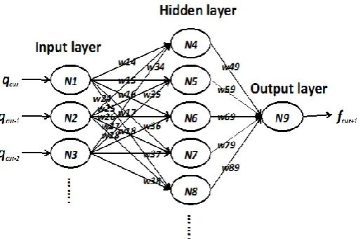
ANNs imitate the structure of the human brain and how it functions for learning and solving problems. Fig. 3 shows the internal structure of a three-layer ANN. An ANN consists of an input layer, zero or more hidden layers, and an output layer. Each layer consists of some number of neurons (e.g., N1, N2, and N3) connected to the neurons in the following layer (N4, …, and N8). With the exception of the neurons in the input layer (i.e., N1, N2, and N3), each ANN neuron has an activation function that determines whether the output connections of that neuron are activated based on weighted inputs coming from the previous layer’s neurons. In an ANN, each neuron-to-neuron connection has a weight (e.g., w14, w15,…), to which a value is assigned during the training process; thus, the input value received by each neuron is a weighted combination of the values transmitted by that neuron’s input connections. Finally, the last layer (the output layer) generates the final result (fcur+1) of an ANN’s internal calculation.

There are many different methods of training an ANN (determining its weights) for time series forecasting. Detailed introductions to ANNs as they are used in the context of time series forecasting can be found in Chapter 9.3 of [13] and in[3], [17].

Fig. 3. The internal structure of a three-layer ANN.

5.

Conventional Statistical Methods

This section introduces the conventional time series methods that are considered for comparison in this paper, with a focus on their predictor formulations (expressions). These methods can be divided into three groups, namely, benchmark methods, regression methods, and state-of-the-art methods. The first group consists of the baseline methods for time series forecasting. Generally, any proposed forecasting approach must at least be more accurate than the benchmark methods; otherwise, it is worthless. The second group is a set of classical regression models that are commonly used in time series forecasting. Finally, the last group consists of two sophisticated, well-developed methods that are currently used for time series forecasting. In theory, the methods in this group should be the strongest competitors for our proposed GP and SVR approaches because they are currently the de facto solutions in the field.

Three baseline time series methods are introduced in this section.

Average method (Ave.). To generate a forecast value (fcur+1), this method simply calculates the mean of all past

observations (q1…cur).

.

Naïve Method (Nai.). This method directly uses the last observed time series value (qcur) as its forecast value

(fcur+1).

.

Drift Method (Dri.). This method is a variant of the naïve method. Its forecast value is the result of the naïve method plus a drift (the second term in the expression), which is the average amount of variation observed in the historical data.

.

A detailed introduction to these benchmark methods can be found in Chapter 2.3 of [13].

5.2.

Regression Methods

Regression is a statistical technique that is used to analyze the relationships between dependent and independent variables. In this paper, we consider four different common time series regression models.

Simple linear regression(SLR). This is the simplest time series regression model:

,

where is the intercept, is the coefficient of the second term, and tis the time point to be predicted (e.g., for

fcur+1, t = cur+1).

Simple non-linear regression(SNR). This is the non-linear version of simple linear regression:

,

where log() is the natural logarithm function and exp() is the natural exponential function. In this model, simple linear regression is used to fit a transformed linear time series that was originally non-linear (but is now linear after the natural logarithm transformation). Other transformation approaches can be applied, but the natural logarithm approach is common because it is simple and intuitive.

Polynomial regression(PR). The model used in polynomial regression is defined as follows:

,

where is the intercept and , , … are the coefficients of the subsequent terms.

Non-linear polynomial regression (NPR). Similar to the relationship between simple linear regression and its non-linear version, this model is the non-linear version of polynomial regression.

.

5.3.

State-of-the-Art Methods

This section introduces the two most commonly used standard solutions in current time series research, namely, ARIMA models and ES methods.

Auto-Regressive Integrated Moving Average (ARIMA) models. These models comprise three components, namely, the Auto-Regressive (AR), Integrated (I), and Moving Average (MA) components. Each component is associated with an order number (p for the AR component, d for the I component, and q for the MA component) that must be determined by analyzing the past observations. ARIMA predictor models are formulated as follows:

,

where and represent the coefficients of the predictor variables, is the current error, and the for j = 0, 1,…, j are the past errors. The first summation represents the AR component of the model, and the second summation is the MA component. The I component is a d-order time differencing (pre-processing) that is applied to the predicted time series before the AR and MA components are fitted. Several well-developed methods are available for determining the values of the order numbers and the coefficients for a given forecasting problem instance, such as the Box-Jenkins algorithm and the Hyndman-Khandakar algorithm. More detailed introductions to ARIMA models can be found in [1] [2] [13] [20] [21].

Exponential Smoothing (ES) methods. ES methods constitute a group of methods, of which the most representative and complete example is the Holt-Winters method. An (additive) Holt-Winters model can be simply expressed as follows:

,

where describes the level of the predicted time series, describes its trend, and describes its seasonality. Because of space limitations, for the formulas for calculating the level ( ), trend ( ), and seasonality ( ) values, readers are referred to Chapter 7.5 of [13], Section 3.1.2 of [19], and [21]. Other ES methods are variants of the Holt-Winters method that lack the trend or seasonality component (or both) or use a multiplicative model. For example, the simple exponential smoothing (SES) method considers only a level component. The ES approach implemented in this study automatically selects the most suitable ES model to use based on an analysis of the predicted QoS time series. Detailed introductions to ES can be found in Chapter 7 of [13] and [21].

6.

Experiments

This section first describes our experimental environment and settings and then presents the experimental results as evaluated using the forecasting accuracy metrics defined in Section 3.2. The experimental results are discussed in detail in Section 7.

6.1.

Experimental Environment

Hardware. All forecasting approaches were implemented and executed on an Apple MAC computer with a 1.3 GHz Intel Core i5 processor and 4 GB of DDR3 RAM running the OS X 10.11.6 operating system.

Library for Support Vector Machines (LIBSVM) [23], [28]. The methods considered for comparison, including the ANN method, were all implemented in R using the forecast package [29].

QoS dataset. Our experiments were performed on the QoS dataset presented in [20], which incorporates ten distinct dynamic QoS time series collected from ten real-world WSs (e.g., Google and Amazon WSs) and has also been employed in other QoS forecasting studies, such as [1] [20]. More detailed descriptions of the dataset can be found in [1] [20]. To generate more problem instances on which to run our experiments, we split each time series into several time series segments (TSs). These TSs were labeled as TS1_1 (segment 1 of time series 1), TS1_2 (segment 2 of time series 1), TS2_1 (segment 1 of time series 2), etc.

Problem configuration. In this paper, the lengths (tral and tesl) of the training dataset (TraQoS) and testing dataset (TesQoS) were set to 500 and 100, respectively (thus, the length of each TS was 600), which means that each trained/fitted QoS predictor was used to predict the QoS values at 100 future time points. Additionally, in this study, each QoS time series in the dataset was split into 10 TSs to run our experiments.

6.2.

Experimental Results

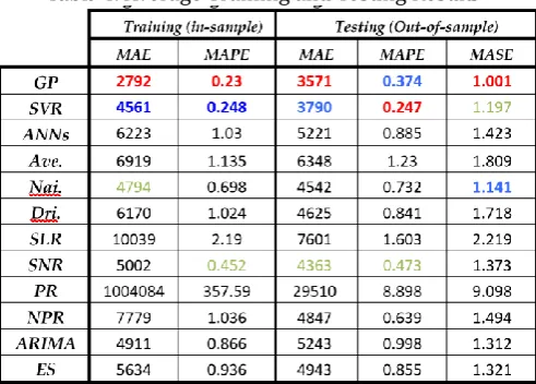
Table 2. The Training (in-sample) MAE Results

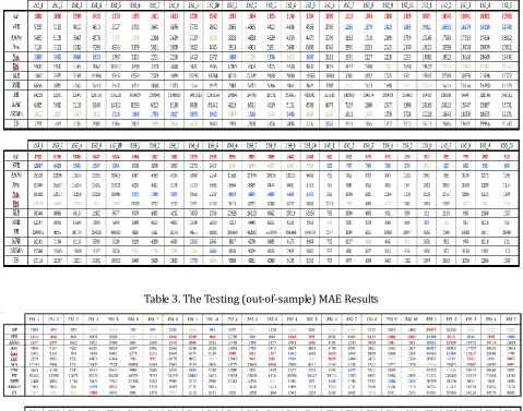
In this section, we present the training (in-sample) and testing (out-of-sample) results obtained in the experiments. For both types of results, the MAE and MAPE measures were calculated, and for the testing accuracy, the MASE was also considered; all measures are defined in Section 3.2. However, because of space limitations, we show only the MAE values for each individual TS experiment. Regarding the MAPE and MASE results, because they are both scale-independent and can be compared across different TSs [14], [15], we present only the average (mean) results for all experiments.

Table 4 lists the training MAE results for the experiments, and the testing MAE results are shown in Table 3. The average results for all experiments are presented in Table 4. For each individual TS experiment in Table 2 and Table 3 and each average result in Table 4, the value corresponding to the best approach (the lowest value) is shown in red, the second-best approach is indicated in blue, and the third-best approach is indicated in green.

Table 4. Average Training and Testing Results

7.

Discussion

This section discusses the experimental results (i.e., Table 2, Table 3, and Table 4) reported in Section 6.2. We analyze first the training performance and then the testing performance achieved in the experiments. From Table 2, it is obvious that GP is superior for all TSs in terms of the training MAE results (i.e., it yields the lowest MAE value in each TS experiment). In addition, Table 4 shows that GP achieves the lowest average values of both the training MAE and the training MAPE. In our experiments, GP is clearly the best-performing approach during the training stage for dynamic QoS time series forecasting. Thus, if the purpose is to accurately model and fit a known QoS time series, GP appears to be the best choice. Regarding the second-best-performing approach during the training stage, Table 2 indicates several competitors, including SVR (which yields the second-lowest MAE value on 23 TSs), Nai. (the second-lowest value on 15 TSs), and ARIMA (the second-lowest value on 9 TSs). Thus, SVR may be considered the winner here because it achieves the second-lowest MAE value on more TSs than either of its two competitors. Moreover, as seen from the average training results reported in Table 4, SVR yields the second-lowest value for both considered measures. These observations suggest that during the training stage, on average, SVR is the second-best-performing approach in our experiments.

performance of a WS.

Regarding the testing accuracy, the results are more complicated because no single approach clearly dominates (achieves the lowest value on each TS and in each measure) according to Table 3 and Table 4. Below, we first present a comparison between the two proposed computational intelligence techniques and then compare these techniques with the conventional time series approaches. In Table 3, SVR achieves the lowest MAE value on 26 TSs; Dri., on 12 TSs; and GP, on 5 TSs. It seems that in contrast to the training results presented in Table 3, GP is inferior to SVR in terms of the testing results shown in Table 3. However, although GP shows the best testing performance on fewer TSs than does SVR, it still yields the best average testing accuracy according to two of the three considered measures (i.e., the MAE and MASE), as seen in Table 4. Among the testing MAE results presented in Table 3, in many of the TS experiments in which SVR outperforms GP, such as TS1_2, TS1_10, TS2_2, TS2_5, TS2_8, TS3_7, TS4_4, TS4_6, TS4_7, TS5_3, TS5_4, TS5_5, TS5_8, and TS5_10, the difference is not significant. However, in experiments TS1_4, TS1_5, TS2_1, and TS4_1, in which GP outperforms SVR in terms of testing performance, SVR yields an MAE value that is two or nearly three times worse than that achieved by GP. This may be the reason why GP outperforms SVR in two of the three average testing measures in Table 4, despite the fact that GP yields the best MAE in significantly fewer experiments. Overall, the superiority of SVR over GP is minor (insignificant) in many cases, whereas the inferiority of SVR compared with GP in some cases is major (significant). Based on the above observations, between GP and SVR, we consider that GP demonstrates a more stable and reliable forecasting capability. An easy way to compare the two proposed computational intelligence techniques with the conventional time series approaches is to consider the average testing accuracy information presented in Table 4. According to this table, both GP and SVR are among the top three best-performing forecasting approaches in terms of all three accuracy measures. In fact, GP and SVR are the top two approaches in all cases except for the average testing MASE, for which SVR is only the third-best-performing approach. Thus, on average, the proposed computational intelligence techniques clearly outperform the other approaches considered for comparison.

Although GP may be the most reasonable choice overall for dynamic QoS time series forecasting, a major cost of using this approach is that GP requires more time to generate a predictor for a given forecasting problem instance because of the time-consuming nature of the evolution process. However, if the forecasting quality is the only concern, GP is still the recommended approach. Otherwise, enhancing the available computation resources and hardware specifications can reduce the time consumed by GP. This problem can also be relieved by using parallel processing platforms provided through the cloud.

8.

Conclusion

significantly higher forecasting errors in several cases, indicating that its performance is unstable and unreliable.

In this paper, we have demonstrated that techniques developed in the field of computational intelligence outperform even the most sophisticated traditional methods of dynamic QoS time series forecasting in services computing. To some extent, this paper can be viewed as a case study of the competition between computational intelligence and traditional disciplines (in this case, statistics and time series forecasting). According to the experimental results presented in this paper, computational intelligence clearly wins the competition in this case.

In the future, we plan to apply computational intelligence techniques to other time series application domains, such as the forecasting of cloud workloads and mobile traffic. Another goal is to enhance the forecasting accuracy of such techniques while simultaneously reducing their cost.

Acknowledgment

This research is partially sponsored by the Ministry of Science and Technology (Taiwan) under the Grant MOST106-2221-E-030-002, MOST106-2811-E-001-003, and MOST106-2221-E-001-007-MY2.

References

[1] Amin, A., Colman, A., & Grunske, L. (2012). An approach to forecasting QoS attributes of web services based on ARIMA and GARCH models. Proceedings of 2012 IEEE 19th International Conference on Web Services (ICWS) (pp. 74-81).

[2] Amin, A., Grunske, L., & Colman, A. (2012). An automated approach to forecasting QoS attributes based on linear and non-linear time series modeling. Proceedings of the 27th IEEE/ACM International Conference on Automated Software Engineering, Essen, Germany.

[3] Zadeh, M. H., & seyyedi, M. (2010). Qos monitoring for web services by time series forecasting. Proceedings of the 3rd IEEE International Conference on Computer Science and Information Technology (ICCSIT) (pp. 659-663).

[4] Huiyuan, Z., Weiliang, Z., Jian, Y., & Bouguettaya, A. (2013). QoS analysis for web service compositions with complex structures. Services Computing, IEEE Transactions on, 6(3), 373-386.

[5] YunNi, X., Jian, D., Xin, L., & QingSheng, Z. (2013). Dependability prediction of WS-BPEL service compositions using petri net and time series models. Proceedings of IEEE 7th International Symposium on Service Oriented System Engineering (SOSE) (pp. 192-202).

[6] Yilei, Z., Zibin, Z., & Lyu, M. R. (2011). WSPred: A time-aware personalized QoS prediction framework for web services. Proceedings of IEEE 22nd International Symposium on Software Reliability Engineering (ISSRE) (pp. 210-219).

[7] Godse, M., Bellur, U., & Sonar, R. (2010). Automating QoS based service selection. Proceedings of IEEE International Conference on Web Services (ICWS) (pp. 534-541).

[8] Iba, H., & Nikolaev, N. (2000). Genetic programming polynomial models of financial data series. Proceedings of the 2000 Congress on Evolutionary Computation (pp. 1459-1466).

[9] Iba, H., & T. Sasaki. (1999). Using genetic programming to predict financial data. Proceedings of the 1999 Congress on Evolutionary Computation (p. 251).

[10] Santini, M., & Tettamanzi, A. (2001). Genetic programming for financial time series prediction. Genetic Programming, 361-370.

[12] Agapitos, A., Dyson, M., Kovalchuk, J., & Lucas, S. M. (2008). On the genetic programming of time-series predictors for supply chain management. Proceedings of the 10th Annual Conference on Genetic and Evolutionary Computation (pp. 1163-1170).

[13] Hyndman, R. J., & Athanasopoulos, G. (2014). Forecasting: Principles and practice. OTexts.

[14] Hyndman, R. J., & Koehler, A. B. (2006). Another look at measures of forecast accuracy. International Journal of Forecasting, 22(4), 679-688.

[15] Hyndman, R. J. Another Look at Forecast-Accuracy Metrics for Intermittent Demand.

[16] Tashman, L. J. (2000). Out-of-sample tests of forecasting accuracy: An analysis and review. International Journal of Forecasting, 16(4), 437-450.

[17] Senivongse, T. , & Wongsawangpanich, N. (2011). Composing Services of different granularity and varying QoS using genetic algorithm. Proceedings of the World Congress on Engineering and Computer Science Lecture Notes in Engineering and Computer Science, San Francisco (pp. 388-393).

[18] Mu, L., Jinpeng, H., & Huipeng, G. (2009). An adaptive web services selection method based on the QoS prediction mechanism. Proceedings of IEEE/WIC/ACM International Joint Conferences on Web Intelligence and Intelligent Agent Technologie (pp. 395-402).

[19] Ye, Z., Mistry, S. K., Bouguettaya, A., & Dong, H. (2014). Long-term QoS-aware cloud service composition using multivariate time series analysis. IEEE Transactions on Services Computing, 99.

[20] Cavallo, B. Penta, M. D., & Canfora, G. (2010). An empirical comparison of methods to support QoS-aware service selection. Proceedings of the 2nd International Workshop on Principles of Engineering Service-Oriented Systems.

[21] Rahman, Z. U., Hussain, O. K., & Hussain, F. K. (2014). Time series QoS forecasting for management of cloud services. Proceedings of the 2014 Ninth International Conference on Broadband and Wireless Computing, Communication and Applications.

[22] Mitchell, T. (1997). Machine Learning. McGraw Hill.

[23] Hsu, C. W., Chang, C. C., & Lin, C. J. (2003). A Practical Guide to Support Vector Classification. [24] Support Vector Machine Regression. Retrieved from http://kernelsvm.tripod.com/

[25] Chen, B. J., Chang, M. W., & Chih-Jen, L. (2004). Load forecasting using support vector machines: A study on EUNITE competition 2001. IEEE Transactions on Power Systems, 19(4), 1821-1830.

[26] Müller, K. R., Smola, A. J., Rätsch, G., Schölkopf, B., Kohlmorgen, J., & Vapnik, V. (1997). Predicting time series with support vector machines. Proceedings of International Conference on Artificial Neural Networks (pp. 999-1004).

[27] Meffert. K. JGAP - Java Genetic Algorithms and Genetic Programming Package. Retrieved from http://jgap.sf.net/

[28] Chang, C. C., & Lin, C. J. (2011). LIBSVM: A library for support vector machines. ACM Transactions on Intelligent Systems and Technology (TIST), 2(3), 27.

[29] Hyndman, R. J. (2015). Forecasting Functions for Time Series and Linear Models. Retrieved from http://github.com/robjhyndman/forecast

Yong-Yi Fanjiang received his MS and Ph.D degree in computer science and information engineering from National Chiao Tung University, Taiwan, in 1998 and from National Central University, Taiwan, in 2004, respectively. Currently, he is an associate professor in the Department of Computer Science and Information Engineering and the chair in the bachelor’s program in software engineering and digital innovation applications, Fu Jen Catholic University, Taiwan. His research interests include mobile and pervasive computing, software engineering, semantic web, and human computer interaction.