SVM-based Automatic Annotation
of Multiple Sequence Alignments
Jiansi Ren∗
School of Computer Science, China University of Geosciences, Wuhan, China Email: [email protected]
Abstract—Multiple Sequence alignments are a critical step in phylogeny inference. There is a lack of an appropriate approach which is capable of 1) finding the best global alignment and 2) automating and reproducing manual editing. Progressive alignment is an effective method for multiple Sequence alignments. However, its application in practice has also long been largely hampered because the alignment regions are not homologous to maximize the alignment score. The standard practice in phylogenetics involves manual editing of alignments and manual editing is a non-trivial task. Aiming at these problems, this study 1) uses SVM to capture the neighborhood of a site to automate and reproduce manual editing, and 2) builds the procedure of SVM Model Training and Automatic Annotation. Experimental results demonstrate that a SVM-based classifier can reproduce the manual editing tasks with an accuracy of 95.5%. This method is stable to both RBF parameters (Gamma and C) and clearly outperforms GBLOCKS and AL2CO, which are conventional editing/annotating methods. The classification accuracy achieved by the proposed method is always much higher than those achieved by the counterpart methods.
Index Terms—Multiple Sequence Alignments, machine learning, automatic annotation
I. INTRODUCTION
Sequence phylogeny is used by biologists to reconstruct the series of events that have led to the distribution and diversity of life. Evolutionary patterns can be found by aligning the sequence of bio-molecules such that homologous positions are aligned into columns.
Biological sequences are supplemented with previously released sequences that are collected from databases using algorithms such as BLAST [1]. Sequence alignments are a critical step in phylogeny inference. However, finding the best global alignment is a computationally complex operation. If a region of the global alignment isn’t properly aligned, the phylogeny reconstruction will attempt to accommodate the erroneously alignment character into the phylogeny, leading to a decrease in resolution. Obtaining biologically accurate alignments is a challenge, as the best methods sometimes fail to align readily apparent conserved motifs [2]. The exhaustive solution has the order of O(nk) where n is the length of the longest sequence and k is the number of sequences, a prohibitive constraint with only a few sequences [3]. Heuristics have been developed, the
most famous of which is probably the progressive alignment method [4].
The progressive alignment algorithm is based on the idea that sequences to be aligned are phylogenetically related and these relationships are used to guide the alignment. Using this approach a tree is inferred by performing alignments [5] between each possible pairs of sequences. The distance between each pairs of sequence is computed as the number of mismatched positions in an alignment divided by the total number of matched position. A neighbor joining [6] “guide tree” is generated from these pair-wise distances, which gives the order of the generation of progressive alignment. The alignment continues with each step treated as a pair-wise alignment between a cluster and the next closest sequence. Gaps are added to an existing multiple sequence alignment and a gap will always be a gap.
A penalty is incurred by introducing and extending a gap. For a linear gap penalty this amounts to scoring each column of the alignment by the sum of the amino acid pair scores in this column. The corresponding score is called the sum of pairs (SP) score [7]. Although progressive alignment enjoys immense popularity and is used in multiple alignment programs like ClustalW [8], it has some weaknesses such as it will attempt to align regions that are not homologous to maximize the alignment score. Furthermore there is no ultimate way of quantifying whether or not the alignment is good.
The standard practice in phylogenetics involves some level of manual editing of alignments. The whole process of manual editing is a time consuming and a non-trivial task. Our aim is to automate and reproduce manual editing using artificial intelligence. The method of choice in this study is neural networks, although we have tested a selection of alternative strategies in the past [9]. In previous work [9], decision tree induction (C4.5), Naïve Bayes, and support vector machine methods were applied to the same dataset. There was no clear winner among the different approaches. SVM [10-13] recorded high precision for the classification of inadequate sites where as for the prediction of valid sites C4.5 was the best. Because the manual editing process often considers the neighborhood of a site, we finally chose to use SVM to capture this important factor.
phylogenetic studies, and 2) to improve the repeatability of the process of editing. We believe that this process may outperform manual editing because it also considers the general phylogenetic structure of the data by using site likelihood computed on a preliminary tree.
The rest of this paper is organized as follows. Section II briefs related work in uses of methods for alignment editing. Section III introduces the methods and the process of implementation. This section also details an application of this system. System accuracy and stability are presented in Section IV. This section also provides a performance evaluation by comparing the approach with the existing editing tools. Section V concludes the paper with a summary.
II. RELATED WORK
Other work have been done on alignment editing: GBLOCKS [14], AL2CO [15] are a few software implementations of alignment editing programs. GBLOCKS is a program that is designed to take as input a multiple protein sequence alignment and perform editing to produce a similarly formatted output with the putative “inadequate” sites removed. GBLOCKS claims to be based on the improvement of phylogenetic results and takes into account homology rather than sequence similarity. While GBLOCKS can function as an alignment editing program and was shown to yield improved results for phylogenetic analysis [14], it is not the one that emulates the manual editing process. The criterion was chosen by the user indicating the amount of variability that will be tolerated at a site. This approach effectively removes columns corresponding to the highest site rates with the argument that they contain multiple hidden substitutions and are then ill-suited for phylogenetic analysis. However, these fast-evolving sites may contain valuable phylogenetic signal to resolve closely related sequences. In the AL2CO implementation, the concept of conservation index was introduced and recommended for use as a parameter for refinement of multiple sequence alignment [15].
Our method was trained on multiple sequence alignments extracted from the PFAM database [16]. About 13,000 sites were classified as valid, inadequate or ambiguous. The latter class was used in the design in hope that the classifier could perceive elements in the alignment that are not obvious to the human eye. Using this annotated corpus, training and testing were performed to create an automated annotator of multiple sequence alignment that can be used for editing.
III. METHODS
This section first addresses the dataset and parameterization. After that, the procedure of SVM Model Training and Automatic Annotation is proposed .
A. Dataset
Thirty-six multiple sequence alignments of protein domains were arbitrarily retrieved from PFAM [16], a database containing a collection of multiple alignments of protein domains or conserved protein regions. A total of
about 13,000 sites of multiple sequence alignments were manually annotated by the authors. Two classes were identified during manual annotation, inadequate and valid sites. Sites were classified as valid where there was evidence that the variability in residue identity within the site was solely due to a substitution process occurring over time. Inadequate sites appeared to be the results of alignment artifacts or contain gap characters for most sequences in the alignment. The natural distribution of the data set is 23%-77% inadequate valid.
B. Parameterization
Five parameters were gathered from the multiple sequences. The first parameter derived from the alignments is called gap ratio g. For each site, we use N-gram analysis (default size=3) and the gap ratio of a site is calculated by dividing the number of N-grams (C) that contain gap characters (-) by the total number of N-grams in the given site (T). Thus, the following equation is used to find the gap ratio.
T C
g= (1)
The possible values of gap ratio, then, lie between 0.00, where none of the sequence in a column have a gap at the site, and 1.00, when all sequences in the column contain a gap character.
The Normalized Site Likelihood Ratio (NSLR) is the site log likelihood (log (l)) considering the data in a column of the alignment, the JTT substitution model [17] and a Neighbor joining tree created from an unedited alignment, minus the site log likelihood (assuming that all sequence are unrelated) of base states picked at random from a set of residues frequencies in the JTT evolutionary model: log (r) normalized by the number of
sequences in the alignment without a gap at that position ((1-g)*t).
t g r l NSLR × − − = ) 1 ( ) log( )
log( (2)
Where, l = site for a given a preliminary tree, r = the site likelihood if the sequences were unrelated (i.e. independent, or random), g = gap ratio, and t = number of sequences. The value of the normalized site likelihood ratio is not bounded, except by zero as a minimum.
Third, parsimony count (PC) is the gap to no-gap transitions given a preliminary tree. The Parsimony count means the minimum number of character changes observed on the tree. The parsimony count was calculated by converting each alignment column into a binary vector (gap/no-gap character). NJ tree was used as a guide to count PC. Site rate, the fourth parameter, is the measure of the rate of evolution at a site relative to other sites in the alignment.
The 4th parameter, site rate, was evaluated using the NJ tree of the unedited alignment, the JTT model and the libcov library [18]. The alpha parameter was estimated from the data.
using the CNG formula [19] for calculating similarity score as follows:
Similarity=
∑
∪
∪ ⎟⎟⎠
⎞ ⎜⎜
⎝ ⎛
+ − ⋅
2 1
2
2 1
2 1
) ( ) (
)) ( ) ( ( 2
D D
g f g f g
g f g
f (3)
where fi(g)=0 if g
∉
D2. Once we got the similarity score,we have NSS=Similarity/T, where T is the total number of grams for the given site. Default size used for
N-gram analysis is 3. For each site, only the next contiguous site was selected to do the similarity analysis.
After parameterization, we have the following output for every multiple sequence alignment and here is an example (Table I):
Alignment file used here is a2m.ann.fta. The first column is the class variable, where 1 indicates a valid site and 0 indicates an invalid site. The 2nd column is gap ratio, the 3rd column is Normalized Site Likelihood Ratio (NSLR), the 4th column is Parsimony Count (PC), the 5th column is the site rates and the last column is the Normalized Similarity Score (NSS).
C. SVM-based Implementation
1) LibSVM package
LibSVM package was employed to build our application. It is an integrated software stack for supporting vector classification, regression and distribution estimation. This package includes source code written in different languages such as C++, Java, Python, Perl, and Matlab and so on.
2) SVM model training
Before doing classification or annotation for a multiple sequence alignment, we need to obtain a model by training our machine learning system [20-22]. The procedure of training a model was illustrated in Fig 1.
In the first place, the training data set was prepared by manually annotating a set of sites and then doing parameterization. The output of our parameterization is then transformed to a standard format (Table II) to feed the SVM application so that we can get a trained model and save it for later use (classification or annotation).
Annotated alignments initially used for model training could be prepared by end user by simply providing a pair of unedited and edited alignment, and then this system will generate the annotated alignment. In this regard, the SVM model could be refined.
TABLE I.
OUTPUT OF A SAMPLE PARAMETERIZATION
class variable gap ratio NSLR PC site rates NSS
1 0.692308 0.517516 0 1.58326 7.3333333
1 0.692308 0.590195 0 2.53675 6.6666667
1 0.769231 0.555369 0.1603 1.19501 4.2314815
1 0.307692 0.649415 0 2.53675 4.0012472
1 0 0.656452 0 2.53675 5.1067823
1 0 0.546849 0.3544 0.927187 2.6718751
0 0 0.53055 0 1.58326 4.3541667
0 0.692308 0 0 2.53675 1.3333333
0 0.692308 0 0.7143 2.53675 2.88
1 0 0.522676 0 0.71405 3.037037
1 0 0.678862 0 0.160314 5.666667
Model Saved/Refined Unedited Alignment
SVM model Training Parameterization Annotated Alignment
Edited Alignment
Figure 2.Procedure of Automatic Annotation.
Figure 3.Example of alignment annotation and editing.
The only difference between this format and the original output of our parameterization is that for each parameter, there is a serial number followed by a colon preceding it.
3) Procedure of Automatic Annotation
Once we have the saved training model, we can build our automatic annotator easily. The procedure of automatic annotation is illustrated in Fig 2. Given an unedited alignment, we did the same process of calculations to get those 5 parameters and fed them to the SVM classifier based on libsvm and loaded the saved model got from the previous step, and then the classifier can predict the classification label for each site, therefore the final annotated alignment or edited alignment will be obtained. An annotation process is to classify each site in an alignment and labelled with its class variable (For instance, “X” indicates a valid site while “C” indicates an invalid site). Here is the example of annotation process as shown in Fig 3.
TABLE II.
STANDARD FORMAT OF PARAMETERIZATION FOR LIBSVM
class variable gap ratio NSLR PC site rates NSS
1 1:0.692308 2:0.517516 3:0 4:1.58326 5:7.3333333
1 1:0.692308 2:0.590195 3:0 4:2.53675 5:6.6666667
1 1:0.769231 2:0.555369 3:0.1603 4:1.19501 5:4.2314815
1 1:0.307692 2:0.649415 3:0 4:2.53675 5:4.0012472
1 1:0 2:0.546849 3:0.3544 4:0.927187 5:2.6718751
0 1:0 2:0.53055 3:0 4:1.58326 5:4.3541667
0 1:0.692308 2:0 3:0 4:2.53675 5:1.3333333
0 1:0.692308 2:0 3:0.7143 4:2.53675 5:2.88
1 1:0 2:0.522676 3:0 4:0.71405 5:3.037037
“C” in class row indicates the corresponding site is invalid while “Z” stands for a valid site. The only difference between an annotated alignment and an edited alignment is that all sites that contain only gap characters which are marked as “C” will be removed from the alignment file.
IV. RESULTS
System accuracy and stability were tested in this section.Experimental results were evaluation by comparison with existing editing tools.
A. System Accuracy
The accuracy of automatic annotation (or site classification) of this system is 95.5% by using 10-fold cross validation testing on the current data set (about 13,000 sites in total).
B. System Stability
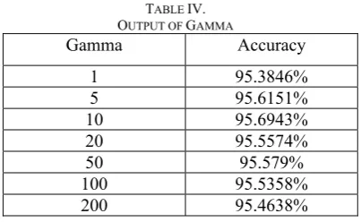
This system was tested by using different combinations of SVM parameters (C, gamma, and Kernel Type and so on). The final Kernel type was used is radical basis function (RBF), since the system performs the best with this kernel type. For RBF kernel, a set of C and gamma were tested and here is the output(Table III, Table IV):
As we can see from the result above, this system is stable for both C and Gamma parameters, since the system accuracy is always around 95.5% with different choices of C or Gamma.
C. Evaluation by Comparison with Existing Editing Tools
As mentioned previously in the introduction section, some existing tools were frequently used to do multiple sequence alignment editing in phylogenetical analysis such as GBLOCKS [14] and AL2CO [15]. To evaluate the performance of our system, the best way is to do comparisons between our application and those existing tools.
1) Comparison with GBLOCKS
Annotation performed by GBLOCKS is to take as input a multiple protein sequence alignment and perform editing to produce a similarly formatted output with the putative “inadequate” sites removed, where valid sites were marked by blue blocks, the rest part of the alignment is considered as inadequate sites as illustrated in Fig 4.
Figure 4.Annotation by GBLOCKS TABLE III.
OUTPUT OF C
C accuracy
1 95.0542% 2 95.1097% 5 95.0859% 10 95.1493% 20 95.1810% 25 95.1889% 50 95.2523% 100 95.2602% 200 95.2840% 500 95.3077% 1000 95.3791% 5000 95.5613% 50000 95.5692%
TABLE IV. OUTPUT OF GAMMA
Figure 5.Information Gain values distribution.
The alignment used here is a2m.ann.fta. The last row in the alignment is our manually annotated class labels (training data) for each site. Blue blocks are the output of GBLOCKS which indicates the corresponding sites are valid sites.
Using GBLOCKS as a classifier, we calculated its accuracy for site classification and here is the result of comparison (Table V). Obviously, our system shows higher accuracies in comparison with GBLOCKS.
The accuracy for the last alignment is higher than our system. This is because GBLOCKS reserves almost all the sites and considers them as valid.
2) Comparison with AL2CO
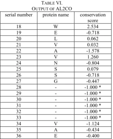
In the AL2CO implementation, the concept of conservation index was introduced and recommended for use as a parameter for refinement of multiple sequence alignment. Here is an example of output by AL2CO as shown in Table VI.
Alignment used here is malic.ann.fta. The first column is the serial number of each site, the second column is the representative protein name for each site and the last column is the conservation score generated by AL2CO.
Since AL2CO didn’t classify each site implicitly, we may use an alternative way to make it a classifier. The idea is to divide the output of AL2Co into 2 groups by choosing a threshold. If the conservation score is higher than the threshold, we then considered it as 1 (valid site) otherwise 0 (invalid site). The problem for this idea is that what the best splitter (threshold) will be?
By taking information theory into consideration, we can figure out a reasonable way of solving this problem:
1. Choose each of these conservation scores as thresholds and build a confusion matrix with four values TP (True Positive), TN(True Negative), FP(False Positive) and FN(False Negative).
2. Calculate information gain (IG) for each threshold using the following formula(Equation 4):
IG=
−
∑
p
ilog
p
i(4)
Where pi=(TP,TN,FP,FN)/(TP+TN+FP+FN) 3. Find the highest value of IG (Fig 5) which is a relatively easy job to do after the IG distribution plot was generated. Choose the conservation score with highest IG as the best threshold and then calculate the corresponding accuracy for the given alignment and compare to that of our system.
Alignment used here is a2m.ann.fta.
Followed the procedure proposed above, we obtained the accuracies for AL2CO as a classifier and here is the result compared to our system (Table VII).
TABLE V.
COMPARISON BETWEEN OUR SYSTEMS TO GBLOCKS
Alignment This work GBLOCKS
a2m.ann 87.3% 39.7%
malic.ann 91.5% 30.6%
MotA_ExbB.ann 90.7% 23.9% aa_permease.ann 91.2% 44.9% bac_export_1.ann 94.7% 21.6% bunya_g1.ann 97.6% 94.56% rubisco_large.ann 96.4% 98.1%
TABLE VI.
OUTPUT OF AL2CO
serial number protein name conservation score
18 W 2.534
19 E -0.718
20 L 0.062 21 V 0.032
22 A -1.578
23 V 1.260
24 N -0.804
25 S 0.079
26 S -0.718
27 G -0.447
28 - -1.000 *
29 - -1.000 *
30 - -1.000 *
31 - -1.000 *
32 - -1.000 *
33 - -1.000 *
34 V -1.124
35 A -0.434
The result above also shows that our system outperforms AL2CO with higher accuracies.
V. CONCLUSIONS
In order to cater for the needs of Multiple Sequence Alignments, this study explores an approach to 1) automate and reproduce manual editing, and 2) enable efficient and scalable Automatic Annotation. The first issue had been addressed using SVM to capture the neighborhood of a site. The Automatic Annotation problem had been tackled by building the procedure of SVM Model Training and Automatic Annotation. Comparison with existing editing tools had been carried out and revealed this method can facilitate the process of multiple alignments annotation. It is stable for both of RBF parameters (c & gamma). This system outperforms some of the existing annotation methods with higher accuracy. Most importantly, this method allows individual users to refine or redefine the training set used to build the classifier by simply providing example pairs of annotated and original MSA in order to reproduce the editing criteria of individual phylogeneticists. This refine/redefine process does not require any knowledge of SVM-based machine learning classification from the end-user. It provides an ideal tool for Multiple Sequence Alignments.
REFERENCES
[1] Altschul, S.F., Gish, W., Miller, W., Myers, E. and Lipman, D. “A basic local alignment search tool, ” J. Mol. Biol., Vol. 215, pp. 403-410, 1990.
[2] Edgar, R.C. “MUSCLE: multiple sequence alignment with high accuracy and high throughput.” Nucleic Acids Res 32(5), 1792-1797, 2004.
[3] Thompson, J.D., Plewniak, F. and Poch, O. “A comprehensive comparison of multiple sequence alignment programs.” Nucleic Acids Research, 27(13), 2682-2690, 1999.
[4] Feng, D. and Doolittle, R. F. “Progressive sequence alignment as a prerequisite to correct phylogenetic trees.” J. Mol. Evol. 60, 351-360, 1987.
[5] Needleman, S. B. and Wunsch, C. D. “A general method applicable to the search for similarities in the amino acid sequence of two proteins.” J. Mol. Biol. 48, 443-453, 1970. [6] Swofford, D.L. and OlsenG.J. “Phylogenetic inference.”
Hillis, D.M., Moritz, C., and Mable, B. (eds.) Molecular Systematics (2nd ed.). 407-514. Sinauer Associates, Sunderland, Massachusetts, 1996.
[7] Gusfield, D. “Algorithms on Strings, Trees, and Sequences.” Cambridge University Press, 1997.
[8] Thompson, J.D., Higgons, D.G. and Gibson, T.J. “CLUSTAL W: improving the sensitivity of progressive multiple alignment through sequence weighting, position specific gap penalities and weight matrix choice.” Nucleic Acids Research, 22(22), 4673-4680, 1994.
[9] Shan, Y., Milios, E.E., Roger, A.J., Blouin, C. and Susko, E. “Automating Recognition of Regions of Intrinsically Poor Multiple Alignment for Phylogenetic Analysis using Machine Learning.” Proceedings of the 2003 IEEE Bioinformatics Conference. 482-483, 2003.
[10]Zhu Fang, Wei Junfang and Shi Wenbo. “SVM Fast Classification Algorithm of Based on Similarity Analysis”, International Journal of Digital Content Technology and its Applications(JDCTA), AICIT, vol. 7, no. 2, pp. 10-16, 2013.
[11]Liqin Fu, Haiguang Zhai, Yongmei Zhang and Dan Yu. “Binary tree SVM –based Emotion Recognition from Speech Signal”, International Journal of Advancements in Computing Technology(IJACT), AICIT, vol. 5, no. 1, pp. 224-232, 2013.
[12]Zheng Xiaomei. “A Novel Method for Foreign Language Teaching Evaluation Based on Feature Selection”, International Journal of Digital Content Technology and its Applications(JDCTA), AICIT, vol. 7, no. 2, pp. 133-140, 2013.
[13]Tao Dongli, Xiao Zhitao, Zhang Fang, Geng Lei and Wu Jun. “Cloth Defect Classification Method Based on SVM”, International Journal of Digital Content Technology and its Applications(JDCTA), AICIT, vol. 7, no. 3, pp. 614-622, 2013.
[14]Castresana, J. “Selection of Convserved Blocks from Multiple Alignments for Their Use in Phylogenetic Analysis.” Molecular Biology and Evolution. 17(4), 540-552, 2000.
[15]Pei, J. and Grishin, N.V. “AL2CO: calculation of a positional conservation in a protein sequence alignment.” Bioinformatics 17(8), 700-712, 2001.
[16]Bateman, A., Coin, L., Durbin, R., Finn, R.D., Hollich, V., Griffith-Jones, S., Khanna, A., Marshall, M., Moxon, S., Sonnhammer, E.L.L., Studholme, D.J., Yeats, C. and Eddy, S.R. “The Pfam protein families database.” Nucleic Acids Research. 32, D138-141, 2004.
[17]Jones,D.T., Taylor,W.R. and Thornton,J.M. “The rapid generation of mutation data matrices from protein sequences.” Comp. Appl. Biosci., 8, 275–282, 1992. [18]Butt, D., Roger, A.J., and Blouin, C. “libcov: A C++
bioinformatic library to manipulate protein structures, sequence alignments and phylogeny.” BMC Bioinformatics, in press, 2005.
[19]Vlado Keselj, Fuchun Peng, Nick Cercone and Calvin Thomas. “N-gram-based Author Profiles for Authorship Attribution” In Proceedings of the Conference Pacific Association for Computational Linguistics, PACLING'03, Dalhousie University, Halifax, Nova Scotia, Canada, 255-264, 2003.
[20]Baldi, P. and S. Brunak. “Bioinformatics: the Machine Learning Approach.” MIT Press, 1998.
[21]Kohavi, R. and Provost, F. “Special Issue on Applications of Machine Learning and the Knowledge Discovery Process”. Machine Learning, 30, 271-274, 1998.
[22]Mitchell, T.M. “Machine Learning.” WCB/McGraw-Hill, 1997.
TABLE VII.
COMPARISON BETWEEN OUR SYSTEM TO AL2CO
Alignment This work AL2CO
a2m.ann 87.3% 55.1%
malic.ann. 91.5% 53.3%
MotA_ExbB.ann 90.7% 52.7% aa_permease.ann 91.2% 54.6% bac_export_1.ann 94.7% 51.0%
Bunya_g1.ann 97.6% 50.1%
Jiansi Ren received the B.Sc. degree from Northeast Normal