Calculation Method of Lateral and Vertical
Diffusion Coefficients in Wide Straight Rivers
and Reservoirs
Zhou-hu WU
Qingdao Technological University, Qingdao Shandong 266033, P. R. China E-mail : [email protected]
Wen WU
Queen's University. Kingston. Ontario, K7L 3N6, Canada E-mail: [email protected]
Gui-zhi WU
Qingdao Technological University, Qingdao Shandong 266033, P. R. China E-mail: [email protected]
The study is financially supported by the National Natural Science Foundation of China (50979036), and by the Foundation of National Water Pollution Control and Governance of China (NO. 2009ZX07210-007-01).
Abstract—In the calculation of mixed-transport capacity of pollutants which were discharged from bank outfall of wide straight rivers or reservoirs, the lateral diffusion coefficient can better demonstrate the mixed-diffusion characteristics near the bank than the transverse diffusion coefficient. For deep rivers and reservoirs, the vertical diffusion coefficient is one of the important water quality parameters. Based on the theoretical calculation method of pollutant mixing zone, the unified equations of the standard curve and curved surface outside the borders of pollutant mixing zone were deduced, including the characteristic parameters of maximum length Ls, maximum width bs and maximum depth ds et al. The shape of curve is akin to semi-elliptic, and the shape of curved surface is akin to part ellipsoid, which is similar to the pollution of the mixing zone. The calculation equation of lateral diffusion coefficient or vertical diffusion coefficient which was determined by the maximum length and maximum width or maximum depth of the outer boundary of pollutant mixing zone near the discharge outfall and the mean velocity were put forward in this paper. The calculation method of the lateral diffusion coefficient or vertical diffusion coefficient which was overall controlled by the area or volume of pollutant mixing zone and the practical method of vertical diffusion coefficient which was determined by the concentration of surface transverse integration was proposed in the paper. The lateral diffusion coefficient of the downstream of Guangfu River in low water season was given, which was 0.27 m2/s by analyzing the data from field observation.
Index Terms—rivers, reservoirs, pollutant mixing zone, standard curve, lateral diffusion coefficient, vertical diffusion coefficient, calculation methods.
I. INTRODUCTION
In the coastal area of rivers and reservoirs, when industrial or domestic sewage are treated to achieve the appropriate discharge standards the waste is discharged along the bank side through the pipes or open channels in most cases. The sewage dilutes and mixes near the outfalls at first, then convects and diffuses along the direction of length, width and depth. Thus the pollutant mixing zones are formed near the sewage outfalls[1]. The distribution of the pollutant mixing zone in wide rivers is mostly two-dimensional problem[2,3]and the distribution in wide deep reservoirs is mostly three-dimensional problem[4,5]. On the other hand, water along the side of rivers and reservoirs is required for high quality to the area of production and living. In large rivers, “total water quality” reaches the standard does not imply that “water quality at bank side” also reaches the standard. “Water quality at bank side” is corresponding to “the environmental capacity at bank”[6].
Transverse and vertical diffusion coefficient of rivers and reservoirs are two of the important water quality parameters to represent the effect of stream to the mixed-transporting capacity of pollutants. The accuracy of parameters is directly related to the reliability of the water quality forecasted in rivers and reservoirs. At present, the prime methods to determine these coefficients are empirical equation method and experimental tracing method. In the empirical method, the dimensionless transverse diffusion coefficient is
*
HU
E
y=
mean water depth in sections, U*: friction velocity) and it
is generally believed that α is 0.3-0.9[7]. So the value of transverse diffusion coefficient is difficult to determine. The tracing experimental method can be divided into field experiments and lab experiments. After that, the moment method[8-12], linear graphical method[13,14], linear regression[15], curve fitting[16], genetic algorithms[17] and artificial neural network[18], etc. can be used to get this transverse diffusion coefficient. Results deduced from field experiment are more reliable, but are restricted by the conditions of injection and sampling of tracers. Lab experiments are commonly used to study the relations between the transverse diffusion coefficient in flumes and roughness, width, water depth, velocity, friction velocity as well as other hydraulic elements. Ref. [19] studied the distribution of transverse turbulence diffusion coefficient in transaction and its equation of mean value with equations of parabolic transaction morphology. Current studies on the equation and value of transverse diffusion coefficient mostly concern about the mixing characteristics in the full-section of rivers. But side discharge is prevalent in practice. The effect of wide rivers and reservoirs (such as the Yangtze River, Yellow River, the Three Gorges reservoir, etc) on the transporting ability of pollutants depends on the mixing diffusion characteristics near the bank primarily. And the calculation of pollutant mixing zone as well as environmental capacity near the bank of large rivers often involves only one-tenth, even one-percent of full-section width. It is obviously unreasonable to adopt transverse diffusion coefficient determined by the hydraulic elements such as average water depth of whole section, the lateral diffusion coefficient can better reflect the mixed-diffusion characteristics near the bank flow than the transverse diffusion coefficient. For example, the average water depth at the Wanzhou section of Three Gorges Reservoir is 71m, but the water depth at the bank is much lower, and it is also in an angular domain formed by a sloping bank.
In this paper, we studied the effect of the flow in wide & deep straight rivers and reservoirs to the mixture and transportation of pollutants. Based on the theoretical calculation method proposed by Ref. [2, 4, 5], deduced the unified equation of the standard curve outside the borders of pollutant mixing zone (isoconcentration) and calculation equations for lateral and vertical diffusion coefficients. The value of lateral diffusion coefficient was calculated by field data of pollutant mixing zone at bank in the Guangfu River. This study provided some reference value for further resolving the calculation of pollutant mixing zone of the large rivers and reservoirs as well as the environmental capacity of bank.
II. CALCULATION OF LATERAL DIFFUSION COEFFICIENT
A. Two-dimensional Problem Of Rivers
The simplified equation of the plane two-dimension advection diffusion of conservative substance in rivers
is U∂C/∂x=Ey∂2C/∂y2 . For a time continuous vertical line source at the bank, the analytic solution for concentration C is:
) 4 exp( π
) , (
2
x E Uy Ux
E H
m y
x C
y y
−
= (1)
Where x is ordinate along the flow direction from the line source, y is transverse perpendicular to x (origin of coordinates locates on the sewage outfall at the bank), m
is discharge strength per unit time, U is average velocity in the bank area, H is average water depth, Ey is
transverse diffusion coefficient of side discharge, named lateral diffusion coefficient.
As it was in Ref. [20], let C=Cd,Cd is allowable
rising value of concentration caused by the river bank blow down,
C
d=
C
s−
C
b where Cs is concentrationstandard and Cb is background concentration practiced in
the water environmental function area. The area encompassed by the isoconcentrate line is pollutant mixing zone.
Therefore, isoconcentrate line equation on the outer boundary of pollutant mixing zone could be deduced from (1) as
⎥ ⎥ ⎦ ⎤ ⎢
⎢ ⎣ ⎡ −
=
m Ux E HC
U x E
y2 4 y ln d π y (2)
Let y in (2) to be zero, we have the theoretical calculation equation of the length of pollutant mixing zone
2 d
s
(
)
π
1
HC
m
U
E
L
y
=
(3)Taking derivative of x in both sides of (2) and letdy dx=0, we can get the calculation equation of maximum width of pollutant mixing zone and its corresponding longitude ordinate. The maximum width of pollutant mixing zone for an outfall at the bank is
U
L
E
UHC
m
b
y se
2
π
e
2
d
s
=
=
(4)Its corresponding longitude ordinate is
e
s c
L
L
=
(5)If we put the (3) and (4) into the (2), the standard curve of the outer boundary of the pollutant mixing zone is deduced as follows:
)
(
ln
e
)
(
2s s
s
L
x
L
x
b
y
−
Or
e
ln
(
)
s s s
L
x
L
x
b
y
=
−
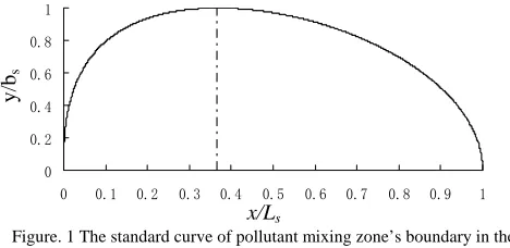
(7)It can be seen from Fig.1 that the shape of the standard curve of pollutant mixing zone’s boundary for an outfall at the bank is nearly semi-ellipse (the standard curve is sy mmetrical ellipse when the pollutant is discharged from ri ver center). There is a blunt area at one end near the outfa ll, while a cusp area appears on the downstream boundary of pollutant mixing zone. The ordinate corresponding to the maximum width of pollutant mixing zone is about 1/e ≈0.368 of the maximum length. This indicates that pollu tant mixing zone has similarity.
Figure. 1 The standard curve of pollutant mixing zone’s boundary in the outfall’s of the bank
The ratio of the maximum length of pollutant mixing zone at the bank side and its width could be given by (4)
2 ePe b
L
s
s = ( 8 )
in which Pe=ULs /Ey is called Peclet number that gives the measure of the rate of longitude advection flux to the lateral diffusion flux of a substance in the flow. So (8) shows the ratio between the pollutant mixing zone’s maximum length and width is proportion to 0.5 order ofPe. We can tell that the Peclet number increases with stronger longitude advection, while the pollutant mixing zone at the bank side is longer and narrower. In contrary cases, the pollutant mixing zone at the bank side is shorter and wider.
Taking definite integral of (7) from 0 to L, we can get the calculation equation of pollutant mixing zone’s area with outfall at the bank as follows,
) d( ) ( ln e
d ) ( ln e
0 0
s L
s s s
s L
s s s
L x L
x L
x b
L
x L
x L
x b
S
s s
∫
∫
− =
− =
(9)
For variables replacement, let x Ls =
ζ
, thenlet
η
=
ζ
1.5, (9) becomesη
η
ζ
ζ
d
)
1
ln(
e
)
3
2
(
d
)
ln(
3
2
e
3
2
1 0 5
. 1
2 3 1
0
2 3
∫
∫
=
=
−s s
s s
b
L
b
L
S
(10)
From the Table of Integral we
know 1 ln( )d π 2
0
1 =
∫
η− η. Replacing the integral in
(10) obtains the analogous semi-ellipse area calculation equation for pollutant mixing zone’s area with outfall at the bank as
s s s
s
b
L
b
L
S
0
.
795
2
π
e
)
3
2
(
1.5=
=
(11)The area coefficient is 0.795 which is only 1.3 % larger than the area coefficient of semi-ellipse (π/4=0.785).
The calculation equation of the lateral diffusion coefficient of wider straight rivers can be given by (3), (4) and (11) which is:
2
2
e
s s
y
b
L
U
E
=
Or 2d s
)
(
π
1
HC
m
UL
E
y=
Or 3
s 2
4
π
27
L
US
E
y=
(12)In practical application, the lateral diffusion coefficient can be calculated by (12) based on the data of field monitoring of pollutant mixing zone by bank.
B. Three-dimensional Problem Of Sloping Bank In Reservoirs
The simplified equation for three-dimension advection diffusion of the conservative substance is U∂C/∂x=Ey∂2C/∂y2+Ez∂2C/∂z2 . If the transverse diffusion coefficient is equal to the vertical diffusion coefficient (Ex=Ey=E), for point source
condition, the analytical solution for isostrength and time-continuous discharge in wider straight reservoirs with sloping bank is:
)
4
)
(
exp(
π
4
2 2
Ex
z
y
U
Ex
m
C
=
β
−
+
(13)Where x is ordinate along the flow direction of reservoirs, y, z are transverse and vertical coordinates perpendicular to x (origin of coordinates locates on the sewage outfall on the surface of water), β is mapping coefficients of the angular domain (β =2πθ, where θ is the included angle between the bank slope and horizontal line), other varieties are same with previous section.
LetC=Cd, the isoconcentrate surface equation of the outer boundary of pollutant mixing zone could be deduced from (13) as
0 0.2 0.4 0.6 0.8 1
0 0.1 0.2 0.3 0.4 0.5 0.6 0.7 0.8 0.9 1
y/
bs
⎭ ⎬ ⎫ ⎩
⎨ ⎧ =
x EC
m U
Ex r
d 2
π 4 ln
4
β
(14)
in which
r
=
y
2+
z
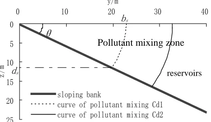
2 . Space shape of isoconcentration surface on the outer boundary of pollutant mixing zone is revolving solid in the bank slope θ. At the transactions where x=const, the isoconcentrate curves on the outer boundary of pollutant mixing zone are the arc corresponding to central angle of θin circular. Fig. 2 shows the x=Lc transaction downstream of theoutfall by the bank of reservoir, in which bs and ds are the
maximum width and length of pollutant mixing zone.
0
5
10
15
20
25
0 10 20 30 40
y/m
z/
m
sloping bank
curve of pollutant mixing Cd1 curve of pollutant mixing Cd2
Figure .2 The section area of the pollutant mixing zone in the outfall’s of the bank downriver x=Lc
We can see from Fig. 2 that calculated based on a three-dimensional time continuous constant point source, the concentration of pollutant could not reach uniformly mixing in depth. In practice when the pollutant discharging at the bank is strong and the pollutant mixing zone is so large that refers to the deep area of reservoir, the analytic solution of three-dimensional convection-diffusion case should be used. When the pollutant discharging is weak and the pollutant mixing zone is just besides the shallow side of reservoir, the analytic solution of two-dimensional convection-diffusion case could be used because the concentration of pollutant is almost uniformly distribute in depth[3].
On the water surface (z=0) of pollutant mixing zone in reservoirs with sloping bank, the theoretical calculation equations of the maximum length Ls and maximum width
bs are[4]:
d s π
4 EC m
L =
β
(15)U
EL
b
ss
e
4
=
(16)Ordinate Lc corresponding to the maximum width of
pollutant mixing zone shore in reservoirs with sloping bank, the calculation equation of area S and the equation of isoconcentration standard curve are same with (5), (11) and (6) & Fig.1 of two-dimensional problem of rivers.
For sloping bank cases, the corresponding ordinates of pollutant mixing zone’s maximum length and width are
same as (15) and (5), that is, both of them are at the transaction of
L
c=
L
se
. Solving with (14), we have the relation between the depth of isoconcentrate surface of pollutant mixing zone and its width at the water surface,y
z
=
sin(
θ
)
( 1 7 )Thus the maximum depth of pollutant mixing zone is
s
s
b
d
=
sin(
θ
)
( 1 8 )Integrating the revolver at angle θ, the volume calcula tion equation for pollutant mixing zone at the bank side is obtained
s 2 0
1 2
4
π
e
d
)
(
ln
π
e
L
b
x
L
x
L
x
b
V
L ss s s
s
β
β
=
=
∫
−(19)
The volume of the pollutant mixing zone by side is β times larger than it is when there is no boundary, which means the existence of boundary constricts the diffusion of pollutant and leads to larger volume of polluted water.
The calculation equation of lateral diffusion coefficient in wider straight reservoirs with sloping bank, from (15), (16) and (11) is:
2 s s
4
e
b
L
U
E
=
Ors d
π
4
C
L
m
E
=
β
Or
3 s
2 3
π ) 2 3 (
L US
E = (20)
In practical application, the lateral diffusion coefficient can be obtained from (20), based on the data of field observation in the pollutant mixing zone of surface of reservoirs with sloping-bank.
C. Three-dimensional Problem In The Reservoirs With Vertical Bank
The simplified equation for three-dimension advection diffusion of the conservative substance is
2 2 2
2 / /
/ x E C y E C z
C
U∂ ∂ = y∂ ∂ + z∂ ∂ . For point
source condition the analytical solution of isostrength time-continuous in wide straight reservoirs with vertical bank is:
)
4
4
exp(
π
2 2
x
E
Uz
x
E
Uy
E
E
x
m
C
z y
z y
−
−
=
(21)Let C=Cd, from Ref. [5], on the water surface (z=0) of pollutant mixing zone in reservoirs with vertical bank the theoretical calculation equation of the maximum length Ls and maximum width bs can be deduced as
follows: bs
Pollutant mixing zone
reservoirs
θ
z y s
E E C
m L
d
π
= (22)
U
L
E
b
s y se
4
=
(23)The theoretical calculation equation of ordinate Lc
corresponding to bs which express maximum width of
pollutant mixing zone shore in reservoirs with vertical bank, area S and the equation of isoconcentration standard curve are same to the (5) , (11) and (6) & Fig.1 of two-dimensional problem of rivers respectively. The calculation equation of lateral diffusion coefficient of wide straight reservoirs can be deduced from (22), (23) and (11) as:
2 s s
4
e
b
L
U
E
y=
Or 3s 2 3
π
)
2
3
(
L
US
E
y=
(24)In practical application, the lateral diffusion coefficient can be obtained from (24), based on the data of field monitoring in the pollutant mixing zone of reservoirs with vertical-bank.
III. CALCULATION OF VERTICAL DIFFUSION COEFFICIENT
Focusing on three dimensional cases in vertical bank reservoirs, further discussions in calculation of vertical diffusion coefficient when it is different from the lateral one are presented in this section.
A. Vertical Transaction Of Pollu-tant Mixing Zone Method
Let C=Cd, at the vertical transaction where y=0, isoconcentrate line equation on the outer boundary of pollutant mixing zone in depth is obtained from (21) as
⎪⎭
⎪
⎬
⎫
⎪⎩
⎪
⎨
⎧
=
d
π
4
ln
4
C
E
E
x
m
U
x
E
z
z y
z
β
( 2 5 )
Taking derivative of x in both sides of (25) and let
0
d
d
z
x
=
, we can see that the corresponding ordinate of pollutant mixing zone maximum depth is the same as (5) in transactiony
=
0
. That means the maximum depth and width of pollutant mixing zone are at the samee
s
c
L
L
=
transaction. Substituting (5) into (25), we have the maximum depth of pollutant mixing zone iss s
s
e
2 b
U L E
d = z =
λ
( 2 6 )in which
λ
=
E
zE
y . From (26) we can see that the ratio of maximum depth and width is proportional to 0.5 order of the ratio λ of vertical and lateral diffusion coefficients in the case that pollutant mixing zone is by the side of reservoirs.If we put (22), (23) and (26) into the (21), the standard curved surface equation of the outer boundary in the pollutant mixing zone is deduced as follows:
) ln( e ) ( ) (
s s 2
s 2
s L
x L
x d
z b
y + =−
( 2 7 )
Space shape of isoconcentration surface on the outer boundary of pollutant mixing zone is nearly quarter-ellipsoid. At the transactions where x=const, the isoconcentrate curves on the outer boundary of pollutant mixing zone is the arc in quadrant Ⅰcorresponding to standard ellipse equation. Fig. 3 gives the region at x=Lc
transaction downstream the outfall, in which bs and ds are
the maximum width and depth of pollutant mixing zone.
0
5
10
15
20
0 10 20 y/m 30 40 50
z/
m
curve of pollutant mixing Cd1 curve of pollutant mixing Cd2
Figure.3 The section area of the mixing zone in the outfall’s of the bank downriver x=Lc
We can tell from Fig. 3 that calculated based on a three-dimensional surface point source convection-diffusion, pollutant mixing zone is mainly close to the surface and the concentration of pollutant could not reach uniformly mixing in depth.
Curve equation for outer boundary of pollutant mixing zone in depth ordinate is obtained from (27) at y=0 transaction as
) ln( e ) (
s s 2
s L
x L
x d
z −
= ( 2 8 )
It is similar with the width equation for outer boundary of pollutant mixing zone at surface as a half ellipse with a wide ending closing to the outfall and a narrow ending downstream.
Using the same method as we did in the area calculation of pollutant mixing zone at surface, we have the pollutant mixing zone area equation at vertical transactions as
s s s
s
z
L
d
L
d
S
0
.
795
2
π
e
)
3
2
(
1.5=
=
(29)Integrating (27) as nearly quarter-ellipsoid we have the pollutant mixing zone volume equation as
s 0
1
16
π
e
d
)
(
ln
4
π
e
L
d
b
x
L
x
L
x
d
b
V
L s ss s s s
s
=
=
∫
−(30) Pollutant mixing zone
reservoirs bs
The volume of the pollutant mixing zone by side is just 1.9% larger than quarter-ellipsoid, 4 times larger than it is when there is no boundary.
Basing on the characteristic length in the equation for outer boundary of pollutant mixing zone at vertical transaction and using the same method at lateral diffusion coefficient calculation, vertical diffusion coefficient equation of straight-wide reservoirs could be obtained from (26) and (29)
2 s s
4
e
d
L
U
E
z=
,3 s
2 3
π
)
2
3
(
L
US
E
zz
=
( 3 1 )In (31), the vertical diffusion coefficient is proportional to the second order of maximum depth at vertical transaction, first order to the mean velocity, and inversely proportional to the first order of maximum length. This means at the same mean velocity, larger depth or vertical area is corresponding to smaller vertical diffusion coefficient. In practical application, vertical diffusion coefficient could be calculated by (31) with the measured results of pollutant mixing zone at the vertical transaction in vertical bank side by reservoir.
B. Volume Method For Pollutant Mixing Zone By Side
Commonly speaking, distribution of pollutant mixing zone by side is not as regular as (27) shows because of the natural geographic shape of the bank. Measurements of maximum depth and vertical area are also not precise because of many reasons. So we could use numerical integration to get the side pollutant mixing zone volume and then obtain vertical diffusion coefficient by general control calculation with the volume.
From (23, 24, 26 and 30) we have the equation for vertical diffusion coefficient as
4 s
2 2 2
2 s
62 . 1 ) π ( 16
L E
V U L
UV E E
y y
z = = ( 3 2 )
In (32), the vertical diffusion coefficient is proportional to the second order of mean velocity and the volume of pollutant mixing zone, inversely proportional to fourth order of the maximum length and first order of lateral diffusion coefficient. This means at the same mean velocity, longer length and larger lateral diffusion coefficient are corresponding to smaller vertical diffusion coefficient; larger volume of pollutant mixing zone is corresponding to larger vertical diffusion coefficient. With the same lateral diffusion coefficient, larger mean velocity or volume means larger vertical diffusion coefficient, while larger length of side pollutant mixing zone means smaller vertical diffusion coefficient.
In practical application, vertical diffusion coefficient could be calculated by (32) with the measured results of pollutant mixing zone at the vertical transaction in vertical bank side by reservoir. Measured qualities include mean velocity, maximum length and volume of
pollutant mixing zone by side, as well as lateral diffusion coefficient calculated by method deduced in section 2.3.
C. Transverse Integral Con-centration At Surface Method
As the conservation law of matter, diffusion in vertical direction will be less if the transverse integral concentration at surface is larger. Therefore, we can get the vertical diffusion coefficient just by transverse integral concentration at surface CwI, regardless of
monitoring concentration in depth.
When
z
=
0
, we can obtain the surface pollutant concentration distribution for three-dimensional time continuous constant surface point source cases at vertical bank reservoir as)
4
exp(
π
2
x
E
Uy
E
E
x
m
C
y z
y
−
=
(33)Integrating (33) with y, the transverse integral concentration at surface CwI is
∫
∫
∞ ∞
−
=
−
=
0
2 0
2 wI
)
4
d(
)
4
exp(
π
2
d
)
4
exp(
π
y
x
E
U
x
E
Uy
Ux
E
m
y
x
E
Uy
E
E
x
m
C
y y
z
y z
y
(34)
For variable replacement as y x E U
y
4
=
η
, andbecause
2
π
d
)
exp(
02
=
−
∫
∞η
η
, we haveUx
E
m
Ux
E
m
C
z
z
π
d
)
exp(
π
2
0
2 wI
=
∫
−
=
∞
η
η
(35)There is no lateral diffusion coefficient Ey in equation
of transverse integral concentration at surface. So we can obtain the transverse integral concentration at surface CwI
by the measured lateral concentration distribution at x0
downstream outfall of vertical bank reservoir, then calculate vertical diffusion coefficient by following equation
2 wI 0
)
(
π
1
C
m
Ux
E
z=
( 3 6 )surface instead of diffusing to the deeper region. Equation (36) is also available for centre outfall cases in reservoir, where the integral region for transverse integral concentration at surface is the total length of the transaction.
Using transverse integral concentration at surface to calculate vertical diffusion coefficient do not need massive measurements in spacing distribution at deep region, which will save lots of time and effort. The measurement of transverse integral concentration at surface should be nearby the maximum width of pollutant mixing zone, because of the higher concentration of pollutant at that transaction and wider distribution which could ensure a better precision.
IV.ANALYSIS OF OBSERVATION RESULTS
Guangfu River originates from Taishan Mountains, flows through Tai'an & Jining Citys, and discharges into the north tip of Nanyang Lake in the Nansi Lake. The drainage area is about 1331 km2. During a survey in the dry season in March, 2005 found that a starch factory let a mass of excessive starch wastewater to Guangfu River near the right bank of Guanghe Road Bridge in Jining City, which formed a clear and identifiable white pollutant mixing zone near the sewage outfall downstream.
Figure. 4 the pollutant mixing zone in the outfall of a starchy factory near the Guangfu River
Fig. 4 shows the field observations figure of pollutant mixing zone in sewage outfall shore of the starch factory. It can be seen that there is obvious white pollutant mixing zone. The maximum length of outer boundary Ls and the
maximum width bs were 32m and 5m respectively. The ordinate Lc corresponding to bs was 12m and mean velocity of pollutant mixing zone was 0.25 m/s. The width of this section in the river was 72m.
As a wider straight river with a good capacity of longitudinal diffusion, the chromaticity of high concentration white pollutant mixing zone in the bank of the Guangfu River is independent from the other side of boundary. substitute Ls and bs into (6), the curve equation of outer boundary of high concentration white pollutant mixing zone (equal chroma) shore of the starch factory can be predicted as follows:
)
32
(
ln
32
e
5
x
x
y
=
−
(37)The theoretical curve of pollutant mixing zone predicted by (37) is shown in Fig. 4. It can be seen that, the theoretical curve obtained from the Ls and bs is in good agreement with the photo of outer boundary of white pollutant mixing zone. What’s more, the theoretical value of Lc corresponding to maximum width is 11.8 m
(Lc=Ls/e) which is close to the observed value 12m. This
indicates that the simplified equation for the plane two-dimension advection diffusion of conservative substance in rivers and the theoretical equation are applicable to the calculation of pollutant mixing zone in Guangfu River. Therefore, the lateral diffusion coefficient of Guangfu River can be calculated by (12):
27
.
0
5
32
2
25
.
0
71828
.
2
2
e
2⋅
2=
×
×
=
=
ss
y
b
L
U
E
m2/sThe data of field monitoring involved in the calculation method of the lateral diffusion coefficient in wide straight rivers and reservoirs are the maximum length, the maximum width of outer boundary at bank of pollutant mixing zone and mean velocity in the pollutant mixing zone area. The field monitoring at existing sewage outfalls is simple, convenient, rapid, flexible and easy to control when the pollutant mixing zone shore is visible clearly. In general case, the simultaneous monitoring of the flow and water quality is necessary. In other words, some sections and vertical lines must be set on the pollution-affected zone upstream and downstream of sewage outfall to monitor velocity and water quality indicators, at the same time; emission strength and hydraulic elements of river hydrology must be recorded. Then series of isoconcentration lines can be obtained from the monitoring data and mean velocity can be
bs
Lc
sewage outfall
Ls
x
y
o
calculated. When the isoconcentration lines fit the standard curve obtained from (6) well, the value of lateral diffusion coefficient can be calculated by (12). At the same time, the relationship among the lateral diffusion coefficient, hydraulic and hydrologic parameters and scale of pollutant mixing zone can be analyzed.
V.CONCLUSIONS
A unified equation of the standard curve and curved surface describing the border of pollutant mixing zone in wide straight rivers and reservoirs is deduced, which includes the characteristic parameters of maximum length
Ls, maximum width bs and maximum depth ds et al. The
shape of standard curve is nearly semi-ellipse, and the shape of curved surface is nearly part ellipsoid, which is similar to the pollution of the mixing zone. The theoretical calculation equations of lateral and vertical diffusion coefficient in wide straight rivers and reservoirs are obtained. It is indicated that Ey or Ez is proportional to
square of the mean velocity and the maximum width or maximum depth of pollutant mixing zone area, but inversely proportional to the maximum length. A practical method that calculate vertical diffusion coefficient by transverse integration concentration at surface is developed in the paper. When Guangfu River is in the low flow season, the lateral diffusion coefficient
Ey in the downstream of this river is estimated as 0.27 m2/s by analyzing the data of field monitoring.
REFERENCES
[1] Zhang Y L, Li Y L. Companion of analytical calculation to the pollutant mixing zone in the outfall’s [M]. Beijing: Ocean Press. 1993.
[2] Wu Z H. The concept and its application of the dimensionless numbers & conform rules by advection-diffusion in the open channel flow [J]. Journal of Qingdao Technological University, 2008a, 29(5):17-22.
[3] Wu Z H, Jia H Y. Analytic method for pollutant mixing zone in river[J]. Advances in Water Science, 2009, 20(4):544-548.
[4] Wu Z H. 3-D Analytic computational method of pollutant mixing zone for reservoir with incline bank[J]. Science & Technology Review, 2008b, 26(18):30-34.
[5] Wu Z H. 3-D analytic computational method of pollutant mixing zone for reservoir with vertical bank[J]. Journal of Xi’an University of Technology, 2009, 25(4):436-440. [6] Huang Z L, Li Y L, Li J X, et al. Water environmental
capacity for the reservoir of Three Gorges Project [J]. Journal of Hydraulic Engineering, 2004, 35(3):7-16.
[7] Fischer H B, Imberger J, List E J, et al. Mixing in inland and coastal waters[M]. 1979, New York: Academic Press, 107-112.
[8] ELDER J W. The diffusion of marked fluid in turbulent shear flow[J]. Fluid Mechanics, 1959, 5 (4): 544-560. [9] LAU Y L, KRISHNAPPAN B G. Transverse dispersion in
rectangular channels [J]. Journal of Hydraulics Division, ASCE, 1977, 103 (10): 1173-1189.
[10]HOLLEY E R, SIEMOUS J, ABRAHAM G. Some aspects of analyzing transverse diffusion in rivers[J]. Journal of Hydraulic Research, 1972, 10(1):27-57.
[11]DEMETRACOPOULOS A C, STEFAN H G. Transverse mixing in wide and shallow river: Case Study[J]. Journal of Environmental Engineering, ASCE, 1983, 109(3):685-697.
[12]ZHOU Y. Study on transverse diffusion coefficient in natural river[J]. Journal of Hydraulic Engineering, 1988, 19(6):54-60.
[13]LIANG X J, LIU Y Y, ZHANG W J, et al. The study of determining the transverse diffusion coefficient of river through the indoor simulation experiments [J]. Journal of Jilin University(Earth Seience Edition), 2004.34(4):560-565.
[14]GUO J Q, ZHANG Y. Linear graphics method for determining the transverse diffusion coefficient of river[J]. Journal of Hydraulic Engineering, 1997, 28(1):62-67. [15]ZHENG P H, GUO J Q. The linear regression method for
determining the transverse diffusion coefficient of river stream[J]. International Journal Hydroelectric Energy, 1999, 17(3):17-19.
[16]LONG B Q, ZHAO S L, ZHOU H Z, et al. The study of environmental hydraulics for Juexi section in Min river— —Transverse diffusion [J]. Journal of Sichuan Normal University (Natural Science), 2001, 24(4):372-374. [17]JIN B M, YANG X H, JIN J L, et al. Real coding genetic
algorithm for determining the transverse diffusion coefficient of river[J]. International Journal Hydroelectric Energy, 2000, 18(1):9-12 .
[18]LONG T R, GUO J S, FENG Y Z, et al. Modulus of transverse diffuse simulation based on artificial neural network[J]. Environmental Science of Chongqing, 2002,24(2):25-28.
[19]Zheng X R, Deng Z Q, Shen J H. Transverse turbulent dispersion coefficient in straight channel[J]. Advances in Water Science, 2002, 13(6):670-674.