Aerodynamic Performance Optimization Of Wind Turbine Blade By Using High Lifting Device

(1)

242 Razeen Ridhwan, Mohamed Alshaleeh, Arunvinthan S

Abstract: In the “Aerodynamic performance of wind turbine blade by using high lifting device” described that different velocity flow of air is passing through the wind turbine blade model and analyze through a numerical simulation that the pressure variation occur at that surface of the model. Before we built wind turbine blade in any strong wind blowing region the aerodynamic flow analysis is must for withstand the strong wind affects. In this chapter, basic nature of winds and types, wind affects through the wind turbine blade, formation of internal pressure and atmospheric boundary layer. This project could be done with the help of so many research papers were taken and followed in the literature review. The main tool we used in the project is CFD, so we gave some introduction about the CFD and how it could be used. Then we compared the results at the different models in different angles having with and without flap in 2D and 3D. We didn’t do any practical oriented models just we design the model in Gambit and analyze in the Fluent.

Keywords: Aerodynamics, Blade with flaps, CLVS α, CD VS α, CP VS X/C, CFD, Flaps, High Lifting devices, Riblets, pressure and velocity

distribution over wind turbine blades, Wind Turbine.

————————————————————

1. Introduction

Wind turbines, like aircraft propeller blades, turn in the moving air and power an electric generator that supplies an electric current. Simply stated, a wind turbine is the opposite of a fan. Instead of using electricity to make wind, like a fan, wind turbines use wind to make electricity. The wind turns the blades, which spin a shaft, which connects to a generator and makes electricity. When you talk about modern wind turbines, you're looking at two primary designs: horizontal-axis and vertical-axis. Vertical-axis wind turbines (VAWTs) are pretty rare. The only one currently in commercial production is the Darrieus turbine, which looks kind of like an egg beater In a VAWT, the shaft is mounted on a vertical axis, perpendicular to the ground. VAWTs are always aligned with the wind, unlike their horizontal-axis counterparts, so there's no adjustment necessary when the wind direction changes; but a VAWT can't start moving all by itself -- it needs a boost from its electrical system to get started. Instead of a tower, it typically uses guy wires for support, so the rotor elevation is lower. Lower elevation means slower wind due to ground interference, so VAWTs are generally less efficient than HAWTs. On the upside, all equipment is at ground level for easy installation and servicing; but that means a larger footprint for the turbine, which is a big negative in farming areas. VAWTs may be used for small-scale turbines and for pumping water in rural areas, but all commercially produced, utility-scale wind turbines are horizontal-axis wind turbines (HAWTs)

As implied by the name, the HAWT shaft is mounted horizontally, parallel to the ground. HAWTs need to constantly align themselves with the wind using a yaw-adjustment mechanism. The yaw system typically consists of electric motors and gearboxes that move the entire rotor left or right in small increments. The turbine's electronic controller reads the position of a wind vane device (either mechanical or electronic) and adjusts the position of the rotor to capture the most wind energy available. HAWTs use a tower to lift the turbine components to an optimum elevation for wind speed (and so the blades can clear the ground) and take up very little ground space since almost all of the components are up to 260 feet (80 meters) in the air.

PROJECT ORGANIZATION

 Chapter 1 deals with the introduction of nature of wind energy and wind turbine parts and its function, basic blade aerodynamics, influence of atmospheric boundary layer, experimental studies, and methodology and project plan.

 Chapter 2 deals with the literature survey on the different papers. Influence of equilibrium atmospheric boundary layer and turbulence parameter on wind turbine on riblet model.

 Chapter 3 deals with the simulation of CFD with introduction, how to works in CFD, methods used to design the model and analyze it, needs to design and create the grid, and grids used in meshing, advantages, limitations and applications of CFD will study in this section.

 Chapter 4 deals with the influence of high lifting device.

 Chapter 5 deals with the pressure and velocity distribution of wind turbine with and without flap in 2D models using CFD.

 Chapter 6 deals with the pressure and velocity distribution of wind turbine with and without flap in 3D models using CFD.

 Chapter 7 deals with the results and discussion in the pressure distribution occur in the wind turbine blade model it has been shown in the graph. In that graph only we clearly know about that pressure variation occurs in that different point. And how this distribution occurs in that blade model then the compared the _________________________________

 Razeen Ridhwan U, M.Tech ( Avionics ), Hindustan University, Chennai, Tamil Nadu, India,

E-mail :- [email protected]

 Mohamed Alshaleeh.M B.E (Aeronautical

Engineering), CAE MODELLER at Ford Technology Services,Chennai, India.

(2)

243 graph as which it is better we used blade without flap

and with flap (in different angle of flap).

 Chapter 8 deals with the conclusion of this project.

 Chapter 9 deals with reference that we took review and discuss in the different papers on the different building models. And also took some of the book that we used in the reference.

METHODOLOGY

AERODYNAMIC PERFORMANCE OPTIMIZATION OF WIND TURBINE BLADE BY USING HIGH LIFTING DEVICE

THEORETICAL

PRACTICAL

INTRODUCTION

LITERATURE REVIEW

INTRODUCTION TO CFD

SIMULATION OF CFD IN 2D

SIMULATION OF CFD IN 3D

RESULTS AND DISCUSSION

REFERENCES

DESIGN THE BLADE MODEL

2D 3D

WIND FLOW ANGLES 5, 10, 15, 20, 25, 30

WITH AND WITHOUT FLAP IN 5, 10, 20, 25, 30

MESHING THE MODEL FREE MESH AND MAPPED MESH

APPLY BOUNDARY CONDITION AT MODEL, INLET AND OUTLET

ANALYZING THE MODEL

SET THE INLET VALUE UNIFORM FLOW

RUN THE SIMULATION ITERATION PROCESS

ANALYZING THE RESULTS Cp AND VELOCITY DISTRIBUTION

COMPLETION OF FLOW ANALYSIS IN WIND TURBINE BLADE MODELS

2. LITERATURE REVIEW

Van Der Hoven and Bechert [30] presented lift characteristics on a 1:4.2 model of Do-228 commuter aircraft model at low speeds; the results show clear evidence of a small increase in lift curve slope (about 1% according to the authors) over the entire a range of –51 to +201 investigated. This slope increase obviously results from reduced boundary layer displacement thickness distributions caused by riblets; essentially riblets lead to a lower viscous decambering effect on the wing. Such a beneficial effect may be expected to be more pronounced on a transonic wing, where the viscous effects play a major role. The sub layers – vortex generators and MEMS technologies which can be used to control flow separation. J.reneaux concluded that Future laminar flow aircraft can, for example, be fitted with wing tip devices and equipped with riblet in the rear part of the wing upper surface. The use of flow control will reduce the system complexity and the structural weight of the aircraft. It is then important to model the effects of sub-layer vortex generators and synthetic jets with the CFD approach. This will allow the gain in performance to be estimated. Gallagher and Thomas explains the drag reduction as coming primarily from a "purely viscous" modification of the sublayer flow, due to the riblet

geometry, that promotes the development of low speed regions within the valley of the grooves in 1984. Kline highlighted the importance of organized deterministic structures in the near-wall turbulence dynamics in 1967.This series of events is usually referred to as the bursting cycle.A. Baron, M. Quadrio and L. Vigevano were discussed about the prediction of turbulent drag reduction by on the boundary layer/ riblets interaction mechanisms. Turbulent drag reduction experienced by ribletted surfaces is the result of both (1) the interaction between riblet peaks and the coherent structures that characterize turbulent near-wall flows, and (2) the laminar sub layer flow modifications caused by the riblet shape, which can balance, under appropriate conditions, the drag penalty due to the increased wetted surface. The latter "viscous" mechanism is investigated by means of an analytical model of the laminar sub layer, which removes geometrical restrictions and allows us to take into account "real" shapes of riblet contours, affected by manufacturing inaccuracies, and to compute even for such cases a parameter, called protrusion height, related to the longitudinal mean flow. By considering real geometries, riblet effectiveness is clearly shown to be related to the difference between the longitudinal and the transversal protrusion heights. A simple method for the prediction of the performances of ribletted surfaces is then devised. The predicted and measured drag reduction data, for different riblet geometries and flow characteristics, are in close agreement with each other. The soundness of the physical interpretation underlying this prediction method is consequently confirmed. Most of them deal with global measurements of effects of riblet on the boundary layer to reduce the drag, but some concerned with the analysis of flow field in the vicinity of and inside the groove. Some preliminary results on the influence of riblet on the structure of a turbulent boundary layer have been discussed by A. Baron and M. Quadrio. Such complex experiments have used particular instrumentation (tunnels with very large turbulent length scales; laser-Doppler anemometry; very small hot wires). A comparison of hot-wire measurements over flat and ribletted wails is described. Details of the experimental apparatus and procedures are given, together with some preliminary results. The test is validated by the calculation of the parameters of the boundary layer, by the comparison of the usual profiles of the stream wise component of the velocity with the available experimental data, and by a conditional analysis of the instantaneous signal. MEAN and RMS profiles for the stream wise component of the velocity evidence, for the riblet plate, an upward shift in law-of-the-wall plots and an overall, small reduction in fluctuation intensities across the boundary layer. Skewness and flatness factors appear to be unchanged. Time series of velocity samples are analyzed by means of power spectra, correlations, and conditional techniques. In particular, the VITA technique, used as an ejection detector, gives results in agreement with previous studies for the flat-plate case, and suggests a moderate increase of the ejection frequency over the riblet surface. Accordingly, the time/space scales of the events appear to be shorter for the riblet-plate flow

3. INTRODUCTION OF CFD

(3)

244 computational mesh to divide up real world continuous fluids

into more manageable discrete sections.

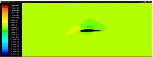
Figure 3.1 (FLOW OVER A 3D BLADE MODEL)

The result of CFD analyses is relevant engineering data used in

 Conceptual studies of new design

 Detailed product development

 Troubleshooting

 Redesign

CFD analysis complements testing and experimentation

 Reduces the total effort required in the laboratory.

4. INFLUENCE OF HIGH LIFTING DEVICE

During the design process of wind turbines it is essential to consider many parameters and influencing variables for example wind velocity, rotational speed, engine performance as well as the resulting drag and lift. Especially the last three parameters are dependent on the surrounding flow field. The turbulence level of the wind field, including the high frequency part, influence the transition of laminar to turbulent flows in the boundary layer. As for the wind field only few results of boundary layer investigation exist under realistic conditions: in the field during rotation. As the experimental set-up is rather complex, most research is conducted in wind tunnels. Due to the lack of detailed experimental results for the flow field including the boundary layer, transition and the influence of high frequency turbulence, simplified and empirical methods are used for the performance prediction of wind turbines.

4.1. AERODYNAMIC ANALYSIS AND DESIGN

PROGRAM

In order to analyze accurately aerodynamic performance of a blade after stall, the information of stall condition is needed. In general, there are few data after stall, we have to calculate the drag and lift coefficients after stall. Generally, a flap device has been used to decrease the length of takeoff and

increase is smaller than that of drag increase. So it is very important to determine the optimum height of a flap for good design. In a three dimensional airfoil of an airplane, tip vortexes are generated due to the pressure difference between the upper and down sides and distribution of circulation surrounding an airfoil decreases. This is the main reason of the loss at a blade tip. A wind turbine also experiences the same phenomena known as blade tip loss.

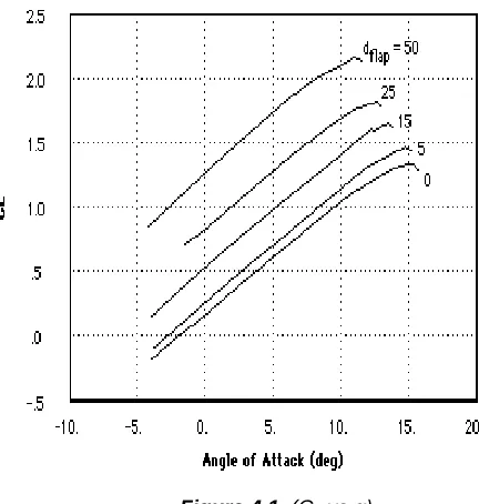
4.2. TYPICAL VARIATION OF FLAPS

Figure 4.1. (CL vs α)

From the above graph we can easily understand how the lift co-efficient (CL) change with the various flaps deflection.

1. Without flap or zero angle deflection of flap the co-efficient of lift is less than 1.5.

2. The flap deflection with 5o co-efficient of lift is near than 1.5 and this value is larger than the co-efficient of lift without flap

3. The flap deflection with 15o co-efficient of lift is more than 1.5 and this value is larger than the co-efficient of lift without flap and also more than c0-efficient of lift at 5o deflection

Flap deflection also produces a large change in lift. From fig4.1 the co-efficient of lift is also increased with the increasing of flap deflection.

5. SIMULATION OF WIND TURBINE BLADE IN

2D

(4)

245 2D and 3D models. So we draw the 2D models in without flap,

flap with 50, 100, -200, 200 & 250deflections.

5.1. CFD SIMULATION FOR FLAP DIFLECTION (2D)

 Without flap

 Flap with 50 deflection

 Flap with -200 deflection

5.1.1. WITHOUT FLAP

Import the NACA4415 aerofoil vertex data in GAMBIT and joint the vertex point and draw the aerofoil by jointing the vertex points. After that create the control area at the dimension of 5C from leading edge in the –ve X direction, 20C from trailing edge in +ve X direction and 5C from chord line to top and bottom of chord line. After the facing process subtract the aerofoil face into control area. Now we got a single face.

Figure 5.1(BLADE WITHOUT FLAP IN 2D)

After the facing process we start meshing the face. First mesh the each line in the model and after finishing the line mesh, mesh the each face mesh. After the meshing process export the model in the “.msh” format. After the modeling the 2D blade we need to analysis the aerodynamic efficiency by using the FLUENT. Read the “.msh” file in the FLUENT and follow the steps which already discussed in chapter3.after finishing the “iterate” process click the contours in display option and see the result of velocity of fluid flow through the model.

Figure 5.2 (MESHED WIND TURBINE BLADE WITHOUT FLAP IN 2D)

Figure 5.3 (VELOCITY DISTRIBUTION OF WIND TURBINE BLADE WITHOUT FLAP IN 2D)

We can understand the velocity distribution over the cross-section of 2D model from the above figure. The maximum velocity occurs on the upper surface of the aerofoil. And for pressure distribution click the contours in display option and see the result of pressure of fluid flow through the model.

(5)

246 pressure occurs on the leading edge of the aerofoil.

5.1.2. FLAP WITH 50 DEFLECTION

Import the NACA4415 aerofoil vertex data in GAMBIT and deflect the 20% of chord length from the trailing edge at 50 downward direction. Now joint the vertex point and draw the aerofoil by jointing the vertex points. After that create the control area at the dimension of 5C from leading edge in the – ve X direction,20C from trailing edge in +ve X direction and 5C from chord line to top and bottom of chord line. After the facing process subtract the aerofoil face into control area. Now we got a single face

Figure 5.5 (BLADE WITH FLAP AT 50 DOWNWARD DEFLECTIONS)

After the facing process we start meshing the face. First mesh the each line in the model and after finishing the line mesh, mesh the each face mesh. After the meshing process export the model in the “.msh” format.

Figure 5.6 (MESHED WIND TURBINE BLADE WITH FLAP

AT 50 DOWNWARD DEFLECTIONS)

After the modeling the 2D blade we need to analysis the aerodynamic efficiency by using the FLUENT. Read the “.msh” file in the FLUENT and follow the steps which already discussed in chapter3.after finishing the “iterate” process click the contours in display option and see the result of velocity of

through the model. We can understand the pressure distribution over the cross-section of 2D model from the below figure 5.8. The maximum pressure occurs on the leading edge of the aerofoil.

Figure 5.7 (VELOCITY DISTRIBUTION OF WIND TURBINE

BLADE WITH FLAP AT 50 DOWNWARD DEFLECTIONS)

Figure 5.8 (PRESSURE DISTRIBUTION OF WIND TURBINE

BLADE WITH FLAP AT 50 DOWNWARD DEFLECTIONS)

Import the NACA4415 aerofoil vertex data in GAMBIT and deflect the 20% of chord length from the trailing edge at 100 downward direction. Now joint the vertex point and draw the aerofoil by jointing the vertex points. After that create the control area at the dimension of 5C from leading edge in the – ve X direction,20C from trailing edge in +ve X direction and 5C from chord line to top and bottom of chord line. After the facing process subtract the aerofoil face into control area. Now we got a single face. After the facing process we start meshing the face. First mesh the each line in the model and after finishing the line mesh, mesh the each face mesh. After the meshing process export the model in the “.msh” format.

FLUID

(6)

247 Figure 5.9 (BLADE WITH FLAP AT 100 DOWNWARD

DEFLECTIONS)

Figure 5.10 (MESHED BLADE WITH FLAP AT 100 DOWNWARD DEFLECTIONS)

After the modeling the 2D blade we need to analysis the aerodynamic efficiency by using the FLUENT. Read the “.msh” file in the FLUENT and follow the steps which already discussed in chapter3.after finishing the “iterate” process click the contours in display option and see the result of velocity of fluid flow through the model.

Figure 5.11 (VELOCITY DISTRIBUTION OF BLADE WITH

FLAP AT 100 DOWNWARD DEFLECTIONS)

We can understand the velocity distribution over the cross-section of 2D model from the above figure5.11. The maximum velocity occurs on the upper surface of the aerofoil. And for pressure distribution click the contours in display option and see the result of pressure of fluid flow through the model.

Figure 5.12 (PRESSURE DISTRIBUTION OF BLADE WITH

We can understand the pressure distribution over the cross-section of 2D model from the above figure 5.12. The maximum pressure occurs on the leading edge of the aerofoil. In the upper surface pressure distribution is very low compare then the lower surface.

Import the NACA4415 aerofoil vertex data in GAMBIT and deflect the 20% of chord length from the trailing edge at 150 downward direction. Now joint the vertex point and draw the aerofoil by jointing the vertex points. After that create the control area at the dimension of 5C from leading edge in the – ve X direction,20C from trailing edge in +ve X direction and 5C from chord line to top and bottom of chord line. After the facing process subtract the aerofoil face into control area. Now we got a single face.

(7)

248 Figure 5.14 (MESHED BLADE WITH FLAP AT 150

DOWNWARD DEFLECTIONS)

FLAP AT 150DOWNWARD DEFLECTIONS)

After the modeling the 2D blade we need to analysis the aerodynamic efficiency by using the FLUENT. Read the “.msh” file in the FLUENT and follow the steps which already discussed in chapter3.after finishing the “iterate” process click the contours in display option and see the result of velocity of fluid flow through the model. We can understand the velocity distribution over the cross-section of 2D model from the above figure5.15. The maximum velocity occurs on the upper surface of the aerofoil and also the minimum velocity occurs the leading and trailing edge of the aerofoil. And for pressure distribution click the contours in display option and see the result of pressure of fluid flow through the model. We can understand the pressure distribution over the cross-section of 2D model from the below figure 5.16. The maximum pressure occurs on the leading edge of the aerofoil and also the minimum pressure occurs on the upper surface at point of deflection starts of the aerofoil. . In the upper surface pressure distribution is low compare then lower surface.

5.1.5.1. FLAP WITH -200 DEFLECTION

Import the NACA4415 aerofoil vertex data in GAMBIT and deflect the 20% of chord length from the trailing edge at 200 upward direction. Now joint the vertex point and draw the aerofoil by jointing the vertex points. After that create the control area at the dimension of 5C from leading edge in the – ve X direction,20C from trailing edge in +ve X direction and 5C from chord line to top and bottom of chord line. After the facing process subtract the aerofoil face into control area. Now we got a single face. After the facing process we start meshing the face. First mesh the each line in the model and after finishing the line mesh, mesh the each face mesh. After the meshing process export the model in the “.msh” format.

Figure 5.17 (BLADE WITH FLAP AT 200 UPWARD DEFLECTIONS)

Figure 5.18 (MESHED BLADE WITH FLAP AT 200 UPWARD DEFLECTIONS)

FLUID

FLOW

(8)

249 After the modeling the 2D blade we need to analysis the

aerodynamic efficiency by using the FLUENT. Read the “.msh” file in the FLUENT and follow the steps which already discussed in chapter3.after finishing the “iterate” process click the contours in display option and see the result of velocity of fluid flow through the model.

Figure 5.19 (VELOCITY DISTRIBUTION OF BLADE WITH FLAP AT 200UPWARD DEFLECTIONS)

We can understand the velocity distribution over the cross-section of 2D model from the above figure5.19. The maximum velocity occurs on the lower surface near the leading edge and trailing edge of the aerofoil and also the minimum velocity occurs on the upper surface near the leading edge of the aerofoil. And for pressure distribution click the contours in display option and see the result of pressure of fluid flow through the model.

Figure 5.20 (PRESSURE DISTRIBUTION OF BLADE WITH FLAP AT 200 UPWARD DEFLECTIONS)

We can understand the pressure distribution over the cross-section of 2D model from the above figure 5.20. The maximum pressure occurs on the leading edge of the aerofoil and also the minimum pressure occurs on the lower surface near the leading edge of the aerofoil. In the lower surface the pressure distribution is very low compare then the upper surface.

5.1.5.2. FLAP WITH 200 DEFLECTION

Import the NACA4415 aerofoil vertex data in GAMBIT and deflect the 20% of chord length from the trailing edge at 200 downward direction. Now joint the vertex point and draw the

aerofoil by jointing the vertex points. After that create the control area at the dimension of 5C from leading edge in the – ve X direction,20C from trailing edge in +ve X direction and 5C from chord line to top and bottom of chord line. After the facing process subtract the aerofoil face into control area. Now we got a single face.

(9)

250 Figure 5.23 (VELOCITY DISTRIBUTION OF BLADE WITH

We can understand the velocity distribution over the cross-section of 2D model from the above figure5.23. The maximum velocity occurs on the upper surface at the point which the starting point of the deflection of the aerofoil and also the minimum velocity occurs the leading and trailing edge of the aerofoil. And for pressure distribution click the contours in display option and see the result of pressure of fluid flow through the model.

We can understand the pressure distribution over the cross-section of 2D model from the above figure 5.24. The maximum pressure occurs on the leading edge of the aerofoil and also the minimum pressure occurs on the upper surface at the point which the starting point of the deflection of the aerofoil. In the upper surface pressure distribution is low compare then lower surface. Here we simulate the wind turbine blade with 20o –ve and +ve deflections. But in the upward (-ve) direction the result was not efficient one that is why we simulate the downward (+ve) in other causes.

5.1.6. FLAP WITH 250 DOWNWARD DEFLECTION

Import the NACA4415 aerofoil vertex data in GAMBIT and deflect the 20% of chord length from the trailing edge at 250 downward direction. Now joint the vertex point and draw the aerofoil by jointing the vertex points. After that create the control area at the dimension of 5C from leading edge in the – ve X direction,20C from trailing edge in +ve X direction and 5C from chord line to top and bottom of chord line. After the facing process subtract the aerofoil face into control area. Now we got a single face.

We can understand the velocity distribution over the cross-section of 2D model from the above figure5.27. The maximum

(10)

251 velocity occurs on the upper surface of the aerofoil and also

the minimum velocity occurs the leading and trailing edge of the aerofoil. And for pressure distribution click the contours in display option and see the result of pressure of fluid flow through the model. We can understand the pressure distribution over the cross-section of 2D model from the below figure 5.28. The maximum pressure occurs on the leading edge and lower surface at the point of deflection of the aerofoil and also the minimum pressure occurs on the upper surface at the point of the aerofoil. In the upper surface pressure distribution is low compare then lower surface.

From this chapter we can clearly understand the upward deflection of flap is not an efficient one so in 3D we go to discus about only downward flap deflection in next chapter.

6. SIMULATION OF WIND TURBINE BLADE IN

2D

In this chapter we will discuss about the aerodynamic efficiency of wind turbine blade in different shapes like normal blade (without flap) and wind turbine blade with flap with different angle of deflection. From the previous chapter (CFD simulation for flap deflection & its aerodynamic efficiency-2D) we know the upward deflection of flap in wind turbine blade is not efficient. So in this chapter we will discuss only about downward deflection of flap. In this chapter we will discuss the aerodynamic efficiency of wind turbine blade without flap, flap with 50 downward deflection and flap with 100 downward deflection.

6.1. CFD SIMULATION FOR FLAP DIFLECTION (3D)

 Without flap

 Flap with 100 downward deflection

 Flap with 200 downward deflection

6.1.1. WITHOUT FLAP

Import the NACA4415 vertex data in different chord length (1.05C at tip of the blade and 2.1C at bottom of blade). The distance between aerofoils was 34.5m. Joint the vertex points and create an aerofoil. Now connect the leading and trailing edges of the aerofoils. This shape looks like an aircraft wing. After the finishing of connection aerofoil we start to draw a cylinder with height 3m and radius 0.5m from the origin (0, 0, and 0). Now we connect the wing to the cylinder (the distance between wing and cylinder is 2.5m). And we get wind turbine blade without flap. After creating the blade model does the

facing process after that does the volume process. Now get a single volume.

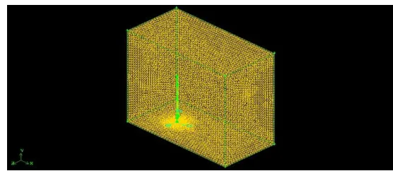
Figure 6.1 (SINGLE VOLUME BLADE)

Now we need to create the control volume with the dimension of height 80m (+ve Y-direction), length 80m (60m from centre of cylinder in the direction of +ve X-direction, 20m from centre of cylinder in the –ve X-direction) and depth 40m (20m in +ve Z-direction and 20m in –ve Z-direction). After finishing the creation of control volume subtract the blade volume into control volume. Now we get a single volume.

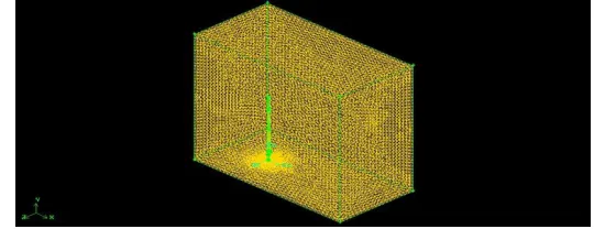
Figure 6.2 (BLADE WITH CONTROL VOLUME)

After finishing the volume process we need do the meshing process. First mesh the each line in the model and after finishing the line mesh, mesh the each face mesh. After finishing the face mesh, mesh the full volume by using volume mesh. After the meshing process export the model in the “.msh” format.

(11)

252 Figure 6.3.b. (MESHED BLADE WITH CONTROL VOLUME)

After the modeling the 3D blade we need to analysis the aerodynamic efficiency by using the FLUENT. Read the “.msh” file in the FLUENT and follow the steps which already discussed in chapter3.after finishing the “iterate” process create the Iso-Surface in distance 3m, 4m, 5.5m, 20m and 40m from origin and click the contours in display option and see the result of velocity of fluid flow through the model.

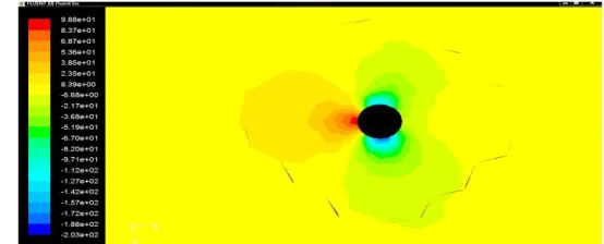
Figure 6.4 (VELOCITY DISTRIBUTION OF BLADE AT 3M)

The figure 6.4 is velocity distribution of Iso-surface of blade in 3m from bottom. In the above figure the maximum velocity occurs on upper and lower surface of circle and the minimum velocity occurs in right and left side of the cylinder.

The figure 6.5 is velocity distribution of Iso-surface of blade in 4m from bottom. It is the in between volume of cylinder and wing. In the above figure the maximum velocity occurs on upper and lower surface and the minimum velocity occurs in trailing edge of the cut section.

Figure 6.6 (VELOCITY DISTRIBUTION OF BLADE AT 5.5M)

The figure 6.6 is the velocity distribution of cut section of blade at 5.5m from the bottom. Here the maximum velocity occurs on the upper surface of the blade and the velocity minimum at leading edge if the blade.

The above figure 6.7 is the velocity distribution of cut section of blade at 20m from the bottom. Here the maximum velocity occurs on the upper surface and other surface in this cut section the velocity is low compare than upper velocity in surface. The below figure 6.8 is the velocity distribution at blade tip. In blade tip normally velocity is more or less same in all faces. And for pressure distribution click the contours in display option and select the Iso-surfaces and see the result of pressure of fluid flow through the model. The below figure 6.9 is pressure distribution of Iso-surface of blade in 3m from bottom. In the above figure the maximum pressure (stagnation pressure) occurs on the leading edge of the cylinder and minimum pressure occurs in upper and lower surface of cylinder.

(12)

253 Figure 6.9 (PRESSURE DISTRIBUTION OF BLADE AT 3M)

Figure 6.10 (PRESSURE DISTRIBUTION OF BLADE AT 4M)

The above figure 6.10 is pressure distribution of Iso-surface of blade in 4m from bottom. In the above figure the maximum pressure (stagnation pressure) occurs on the leading edge of the surface and minimum pressure occurs in upper and lower surface.

Figure 6.11 (PRESSURE DISTRIBUTION OF BLADE AT 5.5M)

The above figure 6.11 is pressure distribution of Iso-surface of blade in 5.5m from bottom. In the above figure the maximum pressure (stagnation pressure) occurs on the leading edge of the aerofoil shape and minimum pressure occurs in upper surface of the aerofoil shape

The above figure 6.12 is pressure distribution of Iso-surface of blade in 20m from bottom. In the above figure the maximum pressure (stagnation pressure) occurs on the leading edge of the aerofoil shape and minimum pressure occurs in upper surface of the aerofoil shape.

Figure 6.13 (PRESSURE DISTRIBUTION OF BLADE AT BLADE TIP)

The above figure 6.13 is the pressure distribution at blade tip. In blade tip normally pressure is more or less same in all faces.

(13)

254 Figure 6.14 (SINGLE VOLUME BLADE WITH FLAP AT 100)

Now we need to create the control volume with the dimension of height 80m (+ve Y-direction), length 80m (60m from centre of cylinder in the direction of +ve X-direction, 20m from centre of cylinder in the –ve X-direction) and dept40m (20m in +ve Z-direction and 20m in –ve Z-direction). After finishing the creation of control volume subtract the blade volume into control volume. Now we get a single volume.

Figure 6.15 (BLADE WITH FLAP 100 DEFLECTEDWITH CONTROL VOLUME)

Figure 6.16.a. (MESHED BLADE WITH FLAP 200 DEFLECTED)

Figure 6.16.b. (MESHED BLADE WITH FLAP 200 DEFLECTEDWITH CONTROL VOLUME)

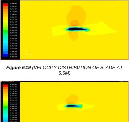
The above figure 6.17 is velocity distribution of Iso-surface of blade in 3m from bottom. In the above figure the maximum velocity occurs on upper surface of circle and the minimum velocity occurs in trailing edge of the cylinder. The below figure 6.18 is velocity distribution of Iso-surface of blade in 4m from bottom. It is the in between volume of cylinder and wing. In the above figure the maximum velocity occurs on upper and lower surface and the minimum velocity occurs in trailing edge of the cut section and in the leading edge velocity also low. The figure 6.19 is the velocity distribution of cut section of blade at 5.5m from the bottom. Here the maximum velocity occurs on the upper surface of the blade and the velocity minimum at leading edge and trailing edges of the blade.

(14)

255 Figure 6.19 (VELOCITY DISTRIBUTION OF BLADE AT

5.5M)

Figure 6.20 (VELOCITY DISTRIBUTION OF BLADE AT 20M)

The above figure 6.20 is the velocity distribution of cut section of blade at 20m from the bottom. Here the maximum velocity occurs on the upper surface and other surface in this cut section the velocity is low compare than upper velocity in surface.

The above figure 6.21 is the velocity distribution of cut section of blade at 32m from the bottom at point which the flap is attached. Here the maximum velocity occurs on the upper surface and other surface in this cut section the velocity is same and low compare than upper velocity in surface.

Figure 6.22 (VELOCITY DISTRIBUTION OF BLADE AT BLADE TIP)

The above figure 6.22 is the velocity distribution at blade tip. In blade tip normally velocity is more or less same in all faces in the tip. And for pressure distribution click the contours in display option and select the Iso-surfaces and see the result of pressure of fluid flow through the model. The below figure 6.23 is pressure distribution of Iso-surface of blade in 3m from bottom. In the above figure the maximum pressure (stagnation pressure) occurs in leading edge of circle and the minimum velocity occurs on trailing upper and lower surface of the cylinder.

FIGURE 6.23 (PRESSURE DISTRIBUTION OF BLADE AT 3M)

(15)

256 Figure 6.25 (PRESSURE DISTRIBUTION OF BLADE AT

5.5M)

The above figure 6.25 is pressure distribution of Iso-surface of blade in 5.5m from bottom. In the above figure the maximum pressure occurs on the leading edge of the aerofoil shape and minimum pressure occurs in upper surface of the aerofoil shape

Figure 6.26 (PRESSURE DISTRIBUTION OF BLADE AT 20 M)

The above figure 6.26 is pressure distribution of Iso-surface of blade in 20m from bottom. In the above figure the maximum pressure occurs on the leading edge of the aerofoil shape and minimum pressure occurs in upper surface of the aerofoil shape.

The above figure 6.27 is the pressure distribution of cut section of blade at 32m from the bottom at point which the flap is attached. Here the maximum pressure occurs on the leading and trailing edges in the upper surface the pressure is very low.

Figure 6.28 (PRESSURE DISTRIBUTION OF BLADE AT BLADE TIP)

The above figure 6.28 is the pressure distribution at blade tip. In blade tip normally pressure is more or less same in all faces.

Import the NACA4415 vertex data in different chord length (1.05C at tip of the blade, 1.293253C at 8m from tip of the blade and 2.1C at bottom of blade). The distance between the tip and bottom aerofoil is 34.5m and distance from the tip to middle aerofoil is 8m. And deflect the middle aerofoil at 100 downward Z-axis (by using copy & rotate).Joint the vertex points and create an aerofoil. Now connect the leading and trailing edges of the aerofoils. This shape looks like an aircraft wing. After the finishing of connection aerofoil we start to draw a cylinder with height 3m and radius 0.5m from the origin (0, 0, and 0). Now we connect the wing to the cylinder (the distance between wing and cylinder is 2.5m). And we get wind turbine blade without flap. After creating the blade model does the facing process after that does the volume process. Now get a single volume.

Figure 6.29 (SINGLE VOLUME BLADE WITH FLAP AT 200)

(16)

257 Figure 6.29 (FLAP 200 DEFLECTED BLADE WITH

CONTROL VOLUME)

Figure 6.30.a. (MESHED BLADE WITH FLAP 200 DEFLECTED)

Figure 6.30.b. (MESHED BLADE WITH FLAP 200 DEFLECTED WITH CONTROL VOLUME)

The above figure 6.31 is velocity distribution of Iso-surface of blade in 3m from bottom. In the above figure the maximum velocity occurs on upper surface of circle and the minimum velocity occurs in trailing edge of the cylinder. Compare than upper surface the velocity is high in lower surface.

Figure 6.32 (VELOCITY DISTRIBUTION OF BLADE AT 5.5M)

The figure 6.32 is the velocity distribution of cut section of blade at 5.5m from the bottom. Here the maximum velocity occurs on the upper surface of the blade and the velocity minimum at leading edge and trailing edges of the blade. The above figure 6.33 is the velocity distribution of cut section of blade at 20m from the bottom. Here the maximum velocity occurs on the upper surface and other surface in this cut section the velocity is low compare than upper velocity in surface. The above figure 6.34 is the velocity distribution of cut section of blade at 30m from the bottom. Here the maximum velocity occurs on the upper surface and other surface in this cut section the velocity is same and low compare than upper velocity in surface.

(17)

30M)

The below figure 6.35 is the velocity distribution of cut section of blade at 35m from the bottom, and in this section flap is attached. Here the maximum velocity occurs on the upper surface and other surface in this cut section the velocity is same and low compare than upper velocity in surface.

The below figure 6.36 is the velocity distribution at blade tip. In blade tip normally velocity is more or less same in all faces in the tip.

And for pressure distribution click the contours in display option and select the Iso-surfaces and see the result of pressure of fluid flow through the model.

The above figure 6.37 is pressure distribution of Iso-surface of blade in 3m from bottom. In the above figure the maximum pressure (stagnation pressure) occurs in leading edge of circle and the minimum velocity occurs on trailing upper and lower surface of the cylinder. The below figure 6.38 is pressure distribution of Iso-surface of blade in 5.5m from bottom. In the below figure the maximum pressure occurs on the leading edge of the aerofoil shape and minimum pressure occurs in upper surface of the aerofoil shape The below figure 6.39 is pressure distribution of Iso-surface of blade in 20m from bottom. In the below figure the maximum pressure occurs on the leading edge of the aerofoil shape and minimum pressure occurs in upper surface of the aerofoil shape.

Figure 6.38 (VELOCITY DISTRIBUTION OF BLADE AT 5.5M)

(18)

30M)

The above figure 6.40 is the pressure distribution of cut section of blade at 30m from the bottom. Here the maximum pressure occurs on the leading and trailing edges in the upper surface the pressure is very low.

The above figure 6.41 is the pressure distribution of cut section of blade at 35m from the bottom, and in this section flap is attached. Here the maximum pressure occurs on the leading and trailing edges in the upper surface the pressure is very low.

The above figure 6.42 is the pressure distribution at blade tip. In blade tip normally pressure is more or less same in all faces. And the pressure is very low on the upper & lower surface of the flap. In this chapter we clearly understand, how the pressure and velocity was varied with & without flap.

7. RESULT AND DISCUSSIONS

In the present work, the using of flap in the wind turbine blade is increasing of lift co-efficient and also the drag co-efficient is increased in little amount. But the amount of drag co-efficient very small with compare then the amount increasing lift co-efficient. Hence there is a sufficient increase in the L/D ratio that is aerodynamic efficiency.In this chapter we will discuss about co-efficient of lift, co-efficient of drag, co-efficient of lift to drag ratio and co-efficient of pressure of the wind turbine model (2D & 3D) with and without flap with different angle of attack (AOA).

7.1. LIFT CO-EFFICIENT FOR 2D MODELS

7.1.1. CL VS α FOR WITHOUT FLAP

Graph 7.1 (CL VS α FOR WITHOUT FLAP)

The above graph is plot co-efficient of lift for different angle of attack. The CL is gradually increased with the angle of attack

increases. From the figure 5.3 the velocity in the upper surface is high. So in the lower surface the pressure is high. Due to the high pressure the lift is created. The lift is increased with the increase of angle of attack.

7.1.2. CL VS α FOR WITH FLAP AT DEFLECTED 5 O

DOWNWARD DIRECTION

Graph 7.2 (CL VS α FOR WITH FLAP AT DEFLECTED 5 O

DOWNWARD DIRECTION)

(19)

260

7.1.3. CL VS α FOR WITH FLAP AT DEFLECTED 10

increases. From the Graph 5.19 the velocity in the upper surface is high. So in the lower surface the pressure is high. Due to the high pressure the lift is created. The lift is increased with the increase of angle of attack. A trailing edge flap is simply a portion of the trailing edge section of the aerofoil that is hinged and which can be deflected downward, as sketched in the insert in Graph 7.3. The positive angle 10o in Graph 7.3, the lift co-efficient is increased (compare the Graph 7.1 & Graph 7.2 with 7.3). This increase is due to an effective increase in the camber of the aerofoil as the flap is deflected downward. In the Graph 7.1 the lift co-efficient is very less at minimum angle of attack -4o (less than 0.1) and in the Graph 7.2 the lift coefficient at minimum angle of attack -4o is near than 0.3 but in Graph 7.3 the lift co-efficient at minimum angle of attack -4o is near than 0.5. It is high compare than blade without flap and also the blade with flap deflected 5o. And also the maximum lift co-efficient of blade without flap is 1.4 at angle of attack +20o. It is also less compare than blade with flap. The maximum lift co-efficient of blade with flap at 10o deflected is more than 1.5 at angle of attack +20o and it is also high compare then the blade with flap deflected 5o. In the Graph 7.3 the lift co-efficient at angle of attack 0o is suddenly deviated (decreased) from our expectation. It may be occurs due to the problem in meshing of the aerofoil or geometrical error or computational problem.

increased with the increase of angle of attack. The positive angle 15o in Graph 7.4, the lift co-efficient is increased (compare the Graph 7.1 & Graph 7.2 with 7.4 but nearly equal to the Graph 7.3). This increase is due to an effective increase in the camber of the aerofoil as the flap is deflected downward. In the Graph 7.4 the lift co-efficient is very high (more than 0.8) at minimum angle of attack -4o with compare than Graph 7.1, 7.2 & 7.3. And also the maximum lift co-efficient more than 1.5 at angle of attack +20o. It is also more than CL of blade without flap, CL of blade with flap with

deflected 5o & CL of blade with flap deflected 10 o

.

)

increases. From the Graph 5.35 the velocity in the upper surface is high. So in the lower surface the pressure is high. Due to the high pressure the lift is created. The lift is increased with the increase of angle of attack. A trailing edge flap is simply a portion of the trailing edge section of the aerofoil that is hinged and which can be deflected downward, as sketched in the insert in Graph 7.5. The positive angle 20o in Graph 7.5, the lift co-efficient is increased (compare the Graph 7.1, 7.2, 7.3 & 7.4 with Graph 7.5). This increase is due to an effective increase in the camber of the aerofoil as the flap is deflected downward. In the Graph 7.5 the lift co-efficient is very high (more than 1) at minimum angle of attack -4o with compare than Graph 7.1, 7.2, 7.3 & 7.4. And also the maximum lift co-efficient more than 1.5 at angle of attack +20o. It is also more than CL of blade without flap, CL of blade

with flap with deflected 5o and also equal to the CL of blade

with flap deflected 10o and CL of blade with flap deflected 15 o

.

(20)

261 The above graph is plot co-efficient of lift for different angle of

attack. The CL is gradually increased with the angle of attack

increases. From the figure 5.39 the velocity in the upper surface is high. So in the lower surface the pressure is high. Due to the high pressure the lift is created. The lift is increased with the increase of angle of attack. A trailing edge flap is simply a portion of the trailing edge section of the aerofoil that is hinged and which can be deflected downward, as sketched in the insert in Graph 7.7. The positive angle 25o in Graph 7.6, the lift co-efficient is increased (compare the Graph 7.1, 7.2, 7.3, 7.4 & 7.5 with Graph 7.6). This increase is due to an effective increase in the camber of the aerofoil as the flap is deflected downward. In the Graph 7.6 the lift co-efficient is very high (more than 1.2) at minimum angle of attack -4o with compare than Graph 7.1, 7.2, 7.3, 7.4 & 7.5. And also the maximum lift co-efficient more than 1.5 at angle of attack +20o. It is also more than CL of blade without flap, CL

of blade with flap with deflected 5o and also equal to the CL of

blade with flap deflected 10o, CL of blade with flap deflected

15o and CL of blade with flap deflected 20 o

increases. From the Graph 5.43 the velocity in the upper surface is high. So in the lower surface the pressure is high. Due to the high pressure the lift is created. The lift is increased with the increase of angle of attack. A trailing edge flap is simply a portion of the trailing edge section of the aerofoil that is hinged and which can be deflected downward, as sketched in the insert in Graph 7.7. The positive angle 30o in Graph 7.7, the lift co-efficient is increased (compare the Graph 7.1, 7.2, 7.3, 7.4, 7.5 & 7.6 with Graph 7.7). This increase is due to an effective increase in the camber of the aerofoil as the flap is deflected downward. In the Graph 7.6 the lift co-efficient is very high (more than 1.4) at minimum angle of attack -4o with compare than Graph 7.1, 7.2, 7.3, 7.4, 7.5 & 7.7. And also the maximum lift co-efficient more than 1.5 at angle of attack +20o. It is also more than CL of blade

without flap, CL of blade with flap with deflected 5 o

and also equal to the CL of blade with flap deflected 10

o

, CL of blade

with flap deflected 15o, CL of blade with flap deflected 20 o

and CL of blade with flap deflected 25

o

7.2. DRAG CO-EFFICIENT FOR 2D MODELS

7.2.1. CD VS α FOR WITHOUT FLAP

Graph 7.8 (CD VS α FOR WITHOUT FLAP)

The above graph is plot co-efficient of drag for different angle of attack. The CD is gradually increased with the angle of

attack increases. From the figure 5.3 the velocity in the upper surface is high. So in the lower surface the pressure is high. Due to the high pressure the lift is created. The lift is increased with the increase of angle of attack. Due to that the flow separation occurs in the trailing edge. So the pressure drag is increased in trailing edge and the skin friction drag increased in the lower surface. The physical source of this drag co-efficient is both skin friction drag and pressure drag due to flow separation (so called from drag). The sum of these two effect yields the profile drag co-efficient CD for the

aerofoil, which is plotted in Graph7.8. The drag is increased with the increase of lift. The wake is created due to the increase of the angle of attack. So the drag is increased. Both CL and CD are increased in the increase of angle of attack

(AOA). In the Graph 7.6 the drag co-efficient at angle of attack 10o is suddenly deviated (increased) from our expectation. It may be occurs due to the problem in meshing of the aerofoil or geometrical error or computational problem.

7.2.2. CD VS α FOR WITH FLAP AT DEFLECTED 5 O

Graph 7.9 (CD VS α FOR WITH FLAP AT DEFLECTED 5 O

(21)

262

7.2.3. CD VS α FOR WITH FLAP AT DEFLECTED 10

The above is the co-efficient of drag for different angle of attack for wind turbine blade with flap at deflected 10o. We can clearly understand the drag increased with increase of angle of attack. In the above Graph 7.10 the drag co-efficient at angle of attack 0o is suddenly deviated (increased) from our expectation. It may be occurs due to the problem in meshing of the aerofoil or geometrical error or computational problem. In the Graph 7.8 the drag co-efficient is very less at minimum angle of attack -4o (less than 0.01) and in the Graph 7.9 the drag co-efficient at minimum angle of attack -4o is near than 0.04 but and in the Graph 7.9 the drag co-efficient at minimum angle of attack -4o is near than 0.05. It is high compare than blade without flap. And also the maximum drag co-efficient of blade without flap deflected with 10o is near than 0.3 at angle of attack +15o. It is also more compare than blade with flap at 5o and blade without flap.

The above is the co-efficient of drag for different angle of attack for wind turbine blade with flap at deflected 15o. We can clearly understand the drag increased with increase of angle of attack. A trailing edge flap is simply a portion of the trailing edge section of the aerofoil that is hinged and which can be deflected downward, as sketched in the insert in Graph 7.11. The positive angle 15o in Graph 7.11, the drag co-efficient is increased (compare the Graph 7.8, Graph 7.9 and Graph 7.10 with Graph 7.11). This increase is due to an effective increase in the camber of the aerofoil as the flap is deflected downward. Due to an effective in the camber the flow separation is also increased. In the increment of flow separation the pressure drag is increased and also the skin

7.2.5. CD VS α FOR WITH FLAP AT DEFLECTED 20 O

The above is the co-efficient of drag for different angle of attack for wind turbine blade with flap at deflected 20o. We can clearly understand the drag increased with increase of angle of attack. A trailing edge flap is simply a portion of the trailing edge section of the aerofoil that is hinged and which can be deflected downward, as sketched in the insert in Graph 7.12. The positive angle 10o in Graph 7.12, the drag co-efficient is increased (compare the Graph 7.8, Graph 7.9 and Graph 7.10 and Graph 7.11 with Graph 7.12). This increase is due to an effective increase in the camber of the aerofoil as the flap is deflected downward. Due to an effective in the camber the flow separation is also increased. In the increment of flow separation the pressure drag is increased and also the skin frictions drag. Then the net drag is increased. So the drag co-efficient is increases with the flow angle of attack. In the above Graph 7.10 CD at -4

o

is more than 0.05 and CD at +15o is 0.3. This result is high compare

than blade without flap, blade with flap at 5o deflected, blade with flap at 10o deflected and blade with flap 15o deflected.

(22)

263 at angle of attack -2o is suddenly deviated (decreased) from

our expectation. It may be occurs due to the problem in meshing of the aerofoil or geometrical error or computational problem. In the above Graph 7.13 CD at -4

o

is more than 0.06 and CD at +15

o

are more than 0.3. This result is high compare than blade without flap, blade with flap at 5o deflected, blade with flap at 10o deflected, blade with flap 15o deflected and blade with flap 20o deflected.

The above is the co-efficient of drag for different angle of attack for wind turbine blade with flap at deflected 30o. We can clearly understand the drag increased with increase of angle of attack. A trailing edge flap is simply a portion of the trailing edge section of the aerofoil that is hinged and which can be deflected downward, as sketched in the insert in Graph 7.14. The positive angle 30o in Graph 7.14, the drag co-efficient is increased (compare the Graph 7.8, Graph 7.9, Graph 7.10, Graph 7.11, Graph 7.12 and Graph 7.13 with Graph 7.14). This increase is due to an effective increase in the camber of the aerofoil as the flap is deflected downward. Due to an effective in the camber the flow separation is also increased. In the increment of flow separation the pressure drag is increased and also the skin frictions drag. Then the net drag is increased. So the drag co-efficient is increases with the flow angle of attack. In the above Graph 7.14 CD at

-4o is more than 0.07 and CD at +15o is more than 0.34. This

result is high compare than blade without flap, blade with flap at 5o deflected, blade with flap at 10o deflected, blade with flap 15o deflected, blade with flap 20o deflected and blade with flap 25o deflected

7.3. LIFT TO DRAG RATIO FOR 2D MODELS

An effective aerofoil produces lift with a minimum of drag; that is, the ratio of lift-to-drag is a measure of the aerodynamic efficiency of an aerofoil. The standard aerofoil have high lift-to-drag (L/D) ratio. And also the co-efficient of lift-lift-to-drag ratio is increased with the angle of attack (AOA). The performance of wind turbine blade is directly proportional to the lift-to-drag ratio (L/D). The Graphs 7.1 to 7.7 show the variation of lift co-efficient versus angle of attack. We see CL increasing linearly

with angle of attack until a maximum value is obtained near 15o, beyond which there is a precipitous drop in lift. The CL

value varies from 0.1 to a maximum of 1.5509, covering a range of angle of attack from -4o to 15o. Many aspects of the flight performance and also our wind turbine blade performance are directly related to the L/D ratio.

Graph 7.15 (LIFT TO DRAG RATIO FOR 2D MODELS)

The Graph 7.15 shows, for a different flap deflection angle. Then that at a given angle of attack, the deflection of flaps increases CL value. On the other hand, the maximum L/D

ratio is increased. Thus, the L/D ratio for a blade without high lifting device (flap) is much small to compare than the blade with high lifting device (flap). Due to the addition of flap in the trailing edge of the wind turbine blade the L/D ratio is increased, we can clearly understand these changes from Graph 7.15. In Graph 7.15 the L/D ratio is increased with increase angle of flap deflected.

7.4. PRESSURE CO-EFFICIENT FOR 2D MODELS

The pressure measurements were carried out for the complete experimental matrix described in an aerofoil section. The results from these measurements are discussed in this section. Typical pressure distribution curves and plots are presented. Graphs (7.16 to 7.22) shows the pressure coefficient curves for the upper and lower surface of the wing, plotted against the percent chord (x/c) for Re=684740 at α=0o

with different flap deflection of the wind turbine blade. Graphs (7.23 to 7.25) presents the same plots for Re = 684740 at α = 5o with different flap deflection of the wind turbine blade, Graphs (7.26 to 7.28) presents the same plots for Re = 684740 at α = 10o

with different flap deflection of the wind turbine blade, Graph 5.4 we can clearly understand the pressure distribution is high at the lower surface of an aerofoil and low at the upper surface of an aerofoil.

Graph 7.16 (CP VS X/C AT AOA 0 o

FOR WITHOUT FLAP)

Graph 7.16 is plot CP vs. X/C of the wind turbine blade without

flap at 0o angle of attack. In the above graph the maximum pressure (stagnation pressure) occurs in the 0th position of X/C that means the stagnation pressure occurs on the leading edge of the wind turbine blade. In the upper the CP is

decrease dramatically to larger negative values. In the upper