Image Reconstruction Using Multi Layer Perceptron (MLP) And Support Vector Machine (SVM) Classifier And Study Of Classification Accuracy

226

Image Reconstruction Using Multi Layer

Perceptron (MLP) And Support Vector Machine

(SVM) Classifier And Study Of Classification

Accuracy.

Shovasis Kumar Biswas, Mohammad Mahmudul Alam Mia

Abstract: Support Vector Machine (SVM) and back-propagation neural network (BPNN) has been applied successfully in many areas, for example, rule extraction, classification and evaluation. In this paper, we studied the back-propagation algorithm for training the multilayer artificial neural network and a support vector machine for data classification and image reconstruction aspects. A model focused on SVM with Gaussian RBF kernel is utilized here for data classification. Back propagation neural network is viewed as one of the most straightforward and is most general methods used for supervised training of multilayered neural network. We compared a support vector machine (SVM) with a back-propagation neural network (BPNN) for the task of data classification and image reconstruction. We made a comparison between the performances of the multi-class classification of these two learning methods. Comparing with these two methods, we can conclude that the classification accuracy of the support vector machine is better, and algorithm is much faster than the MLP with back propagation algorithm.

Index Terms: Neural networks, Classification, Support Vector Machine, Kernel functions, Multi layer perceptron.

————————————————————

1

I

Today, support vector machines and alongside other learning based-kernel algorithm show preferred comes about over multilayer perceptron using back propagation neural networks and other intelligent models. In addition, support vector machines don't depend so intensely on heuristics, i.e. a discretionary decision of the model and have a more adaptable structure [1-2]. Classifying data has been one of the major parts in machine learning. The idea of Support Vector Machine (SVM) is to create a hyper plane in between data sets to indicate which class it belongs to [3-4]. SVM map a given set of binary labelled training data to a high dimensional feature space and separate the two classes of data with a maximum margin of hyper plane. SVM uses an optimum linear separating hyper plane to separate two sets of data in a feature space. The separating hyper plane is the hyper plane that maximizes the distance between the two parallel hyper planes [5]. This optimum hyper plane is produced by maximizing minimum margin between the two sets. Therefore the resulting hyper plane will only be depended on border training patterns called support vectors. So, Support vectors are the data points that lie closest to the decision surface [6]. The neural systems may be viewed as the universal classification of the measured information in the multi-dimensional space [7]. They understand two sorts of characterization: the global and neighborhood one [8].

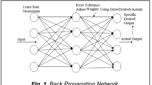
The most vital case of global system is the Multi-Layer Perception (MLP), utilizing the sigmoid enactment capacity of neurons. A typical multilayer perceptron (MLP) network consists of a set of source nodes forming the input layer, one or more hidden layers of computation nodes, and an output layer of nodes. The input signal propagates through the network layer-by-layer. The signal-flow of such a network with two hidden layer is shown in Figure 1. Multi layer feed forward back propagation algorithm is used to train the network and tests the performance of the network. MLP networks are typically used in supervised learning problems [9]. This means that there is a training set of input-output pairs and the network must learn to model the dependency between them. Multilayer Perceptron (MLP) network is a popular learning algorithm in a sense that neural network knows the desired output and adjusting of weight coefficients is done in such way, that the calculated and desired outputs are as close as possible [10-11]. The most illustrative sample of local neural system is the Support Vector Machine (SVM) of distinctive kernel functions. Choosing distinctive kernel functions will produce different SVMs and may result in different performances [12-13]. In the SVM literature, there are four types of kernel function is used, there exist linear kernel, polynomials kernel, sigmoid kernel and RBF kernel. In these popular kernel functions, RBF is the main kernel function because of following reasons [1]: The RBF kernel nonlinearly maps samples into a higher dimensional space unlike to linear kernel, the RBF kernel has less hyper parameters than the polynomial kernel and the RBF kernel has less numerical difficulties. Once the kernel is fixed, SVM classifiers have only a user-chosen parameter called cost parameter. Several survey papers on comparing SVMs with Gaussian Kernels to Radial Basis Function Classifiers can be found in literature, but these focus on a sub-set of techniques and often only on performance accuracy [14-17]. The rest of this paper is organized as follows: Section 2 describes a brief overview on SVM for data classification aspect with SVM program procedure. The multi-layer perception with back propagation algorithm including BPN program training and testing process is described in Section 3. The experimental results are presented in section 4. Also ______________________________

 Shovasis Kumar Biswas is a PhD student at McMaster University, Department of Electrical and Computer Engineering. E-mail: [email protected]

 Mohammad Mahmudul Alam Mia is a Senior Lecturer at Department of Electronics & Communication Engineering, Sylhet International University, Sylhet-3100, Bangladesh.

227 Section 4 gives comparison results between support vector

machines and multi-layer perception classifier. Our conclusion and forthcoming research are presented in Section 5.

2

O

S

V

M

SVM utilizes an optimum linear separating hyperplane to separate two data sets in a feature space. This optimum hyperplane is produced by maximizing minimum margin between the two sets [18]. Therefore the resulting hyperplane will only be depended on border training patterns called support vectors. The support vector machine operates on two mathematical operations: (1) Nonlinear mapping of an input vector into a high-dimensional feature space that is hidden from both the input and output. (2) Construction of an optimal hyperplane for separating the features.

2.1 Variable Definition

1. Let x denote a vector drawn from the input space, assumed to be of dimension 𝑚0.

2. Let 𝜑𝑗 𝑥 for j=1 to 𝑚1, denote a set of nonlinear transformations from the input space to the feature space (Ng & Gong 2002).

3. m1 is the dimension of the feature space.

4. 𝑤𝑗 for j=1 to 𝑚1 denotes a set of linear weights connecting the feature space to the output space.

5. 𝜑𝑗 𝑥 represent the input supplied to the weight 𝑤𝑗 via the feature space.

6. b is the bias.

7. 𝛼𝑖 is the Lagrange coefficient. 8. 𝑑_𝑖 corresponding target output.

2.2 Kernel Selection of SVM

Training vectors xi are mapped into a higher (may be infinite) dimensional space by the function φ. Then SVM finds a linear separating hyperplane with the maximal margin in this higher dimension space. C > 0 is the penalty parameter of the error term [19]. Furthermore, K x, xi = φT x 𝜑 𝑥𝑖 is called the kernel function. There are many kernel functions in SVM, so how to select a good kernel function is also a research issue. However, for general purposes, there are some popular kernel functions [20-21]:

1. Linear kernel:

K x, xi = xTxi

2. Polynomial kernel:

K x,xi = (γxTxi+r)d,γ>0

3. RBF kernel:

K x,xi =exp −γ x−xi 2 ,γ>0

4. Sigmoid kernel:

K x,xi =tanh⁡(γxTxi+r)

Here,𝛾, r and d are kernel parameters. In these popular kernel functions, RBF is the main kernel function because of following reasons [21-22]:

1. The RBF kernel nonlinearly maps samples into a higher dimensional space unlike to linear kernel.

2. The RBF kernel has less hyper parameters than the polynomial kernel.

3. The RBF kernel has less numerical difficulties.

2.3 Steps Involved in the Design of SVM

1. Hyperplane acting as the decision surface is defined as

αidiK x,xi =0 N

i=1 Where

𝐾 𝑥, 𝑥𝑖 = 𝜑𝑇 𝑥 𝜑 𝑥𝑖 represents the inner product of two vectors induced in the feature space by the input vector x and input pattern 𝑥𝑖 pertaining to the ith example. This term is

referred to as inner-product kernel [6], [23].

Where

W= αidiφ xi N

i=1

φ x = [φ₀ x ,φ₁ x , … … . . ,φ_m 1(x)]

T

𝜑0 𝑥 = 1 for all 𝑥 𝑤0 denotes the bias b

2. The requirement of the kernel K x,xi is to satisfy Mercer’s theorem. The kernel function is selected as a polynomial learning machine.

K x,xi = (1+xTxi)2

3. The Lagrange multipliers 𝛼𝑖 for i = 1 to N that maximize the objective function 𝑄 𝛼 , denoted by 𝛼0,i is determined.

Q α = αi− 1

2 αiαjdidjK(x,xi) N

j=1 N

i=1 N

i=1

Subject to the following constraints:

αidi=0 N

i=1 0 ≤ 𝛼_𝑖≤ 𝐶 for i =1,2,…., N

4. The linear weight vector w0 corresponding to the optimum values of the Lagrange multipliers are determined using the following formula:

w0= α0,idiφ(xi) N

i=1

φ(xi) is the image induced in the feature space due to xi. w0 represents the optimum bias b0.

2.4 SVM Program Procedure

Step 1: Read the Image and convert to the Binary Image Step 2: Read 7000 random pixel of Binary Image and keep the pixel value (1 for white, 0 for black)

Step 3: Train the SVM and show the output Step 4: Consider the RBF kernel

Step 5: Classify an observation using a Trained SVM Classifier Step 6: Use cross-validation to find the best parameter rbf_sigma and boxconstraint.

Step 7: Use the best parameter rbf_sigma and boxconstraint to train the whole training set

Step 8: Test and Evaluate the performance of the classifier.

3

B

P

A

228 implementable on a computer [9]. During the training session

of the network, a pair of patterns is called input pattern and desired pattern. The input pattern causes output responses at each neurons in each layer and, hence, an output ok at the output layer. At the output layer, the difference between the actual and target outputs yields an error signal. This error signal depends on the values of the weights of the neurons in each layer [24]. This error is minimized, and during this process new values for the weights are obtained. The speed and accuracy of the learning process that is, the process of updating the weights-also depends on a factor, known as the learning rate.

The process then starts by applying the first input pattern and the corresponding target output. The input causes a response to the neurons of the first layer, which in turn cause a response to the neurons of the next layer, and so on, until a response is obtained at the output layer. That response is then compared with the target response; and the difference (the error signal) is calculated. From the error difference at the output neurons, the algorithm computes the rate at which the error changes as the activity level of the neuron changes. So far, the calculations were computed forward (i.e., from the input layer to the output layer). Now, the algorithms steps back one layer before that output layer and recalculates the weights of the output layer (the weights between the last hidden layer and the neurons of the output layer) so that the output error is minimized [25]. The algorithm next calculates the error output at the last hidden layer and computes new values for its weights (the weights between the last and next-to-last hidden layers). The algorithm continues calculating the error and computing new weight values, moving layer by layer backward, toward the input. When the input is reached and the weights do not change, (i.e., when they have reached a steady state), then the algorithm selects the next pair of input-target patterns and repeats the process [26]. Although responses move in a forward direction, weights are calculated by moving backward. Hence the name of the algorithm is back-propagation.

3.1. Implementation of Back- Propagation Algorithm

The back-propagation algorithm consists of the following steps:

1. Initialization: At first the algorithm has to be initialized considering no prior information is known and picking the synaptic weights and thresholds from a uniform distribution. The type of activation function is sigmoid. 2. Presentations by Training Examples: The network has

to be presented by epochs of training examples to

perform forward and backward computations.

3. Forward Computation: Let us consider, the input vector to the layer of sensory nodes is x(n) and the desired response vector is d(n) which is in the output layer of computation nodes. In forward computation, the network’s local fields and function signals are computed by proceeding forward through the network by layer by layer basis. If sigmoid function is used, the output signal is obtained by the equation below:

y_j l = φ_j(vj(n))

If l=1 which means the j neuron is in the first hidden layer then we get,

y_j 0 =xj(n)

Here, 𝑥_𝑗 𝑛 is the jth element of the input vector x(n).

Let, L is the depth of network. If the neuron j is in the output layer that means l= L then

y_j L =o_j(n) So the error signal will be

ej n = dj n −oj(n)

Here, 𝑑𝑗 𝑛 is the jth element of the vector of desired response d(n).

4. Backward Computation: In backward computation the local gradients of the network is calculated by the following equation (Haykin, 2008):

δj l

n =

e_jL _{n φ} j ′ _{n v}

j

L _{n outputlayerL}

φ_j′ _v j

i _{n δ} k i+1

n w_kj i+1 n k

hiddenlayerl

𝜑𝑗′(·) represents differentiation with respect to the argument. The synaptic weights of the network in layer l have to be adjusted according to the generalized data rule. If η is the training –rate parameter and α is the momentum constant, we get,

w_jil n+1 =w_ji(l) n +∝ w l _ji n−1 +ηδ_j l n y_i l−1 (n) 5. Iteration: Finally the forward and backward computations have to be iterated until the chosen stopping criterion is met. As the number of iterations increases the momentum and learning-rate parameters are adjusted by decreasing the values.

4

E

Our given image is RGB image which is shown in Fig. 2. For our work, we first convert RGB image to gray scale image and then gray scale image to binary image.

Step 1: Boundary Determination and Curve Fitting

229 at the top left corner of the given picture. The (0, 0) point in the

matlab simulation output of our project should be the bottom left corner. In order to produce the boundary lines effectively and efficiently, curve fitting is employed.

Step 2: Training Data Set and Testing Data Set Determination

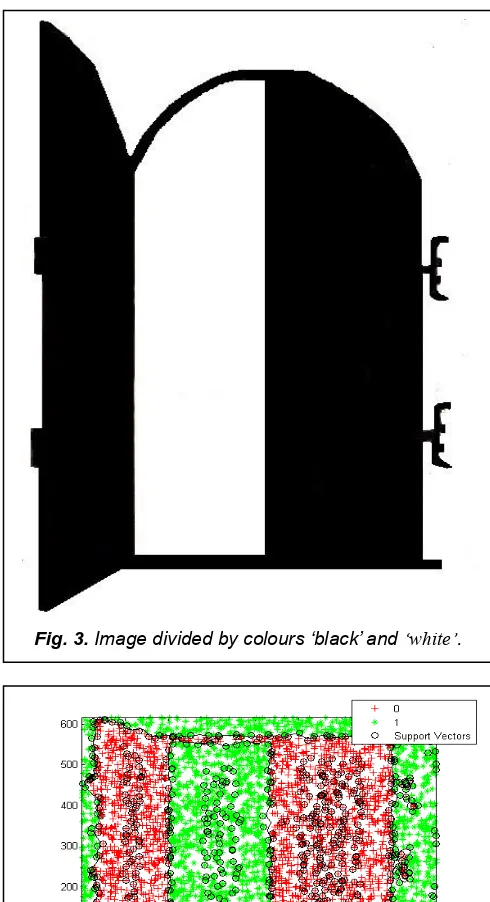
After we have the boundaries of the wooden part of the door with frame, the next step is to obtain points from the original picture and sort the points by colour (black and white). First of all, 252353 points are obtained uniformly from the picture with a resolution of 409×617 pixels. Then, all the points in the wooden part of the door with frame is set as ―0‖ and the colour is set as black. Similarly, all the rest points are set as ―1‖ and the colour is set as white. So after this procedure, a 252353× 3 matrix is generated as the database for our test.

The first two columns represent the X ordinate and Y co-ordinate of a certain point. The third column of the matrix represents the colour of the certain point. For training data set we randomly select 7000 points from 252353 points.

Step 3: Simulation Results

(1) SVM method

In MATLAB software, we used 10-fold cross-validation to find the best parameter rbf_sigma and boxconstraint. At first, we take 7000 samples, divide them into 10 groups of 700 samples each. Then train the network with 9 groups (6300 samples) and test with 1 group (700 samples). This is repeated ten times in matlab simulation, with each group used exactly once as a test set. Finally the 10 results from the folds are averaged

to produce a single output. The results confirmed that the classification precision of the SVM with radial function (RBF) kernel function was as high as 99.5% when rbf_sigma and boxconstraint where 0.0373 and 0.0099. Then we used the best parameter rbf_sigma and boxconstraint to train the whole training set. The outputs from Matlab software are:

Classification Accuracy = 99.5%

(2) MLP method

In this paper, we used multilayer perceptron to train the network with back-propagation algorithm. The number of hidden layers is two, and the number of hidden neurons is 51 and 15 respectively. From the training window, we can access

Fig. 4. Output of the SVM after 10 Cross Validation. Fig. 3. Image divided by colours ‘black’ and ‘white’.

230 three plots: performance, training state, and regression. The

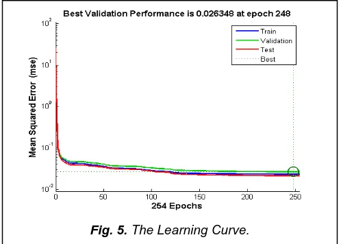
performance plot shows the value of the mean squared error versus the iteration number. Every cycle of the complete preparing set is called an epoch. In every epoch, the network adjusts the weights in the direction that diminishes the error. As the iterative methodology of incremental modification proceeds with, the weights gradually converge to the optimal set of values. Numerous epochs are generally needed before training is completed. Training automatically stops when Mean Square Error (MSE) of the validation samples is increased. The average squared difference between outputs and targets is called the Mean Squared Error (MSE). Lower value of mean squared errors is better while zero means no error. The regression plot shows the relationship between the outputs of the network and the targets. Regression plot is used to validate the neural network. Regression analysis is performed to measure the correlation between outputs and targets. If the training were perfect, the outputs and the targets would be precisely equivalent, and however the relationship is seldom impeccable in practice.

For this implementation, the data set is collected from the given picture and Levenberg-Marquardt back-propagation algorithm is used for training the network. The performance of the proposed network is trained with back-propagation algorithm using MATLAB R2013a that is shown in Fig. 5. We ran the back- propagation algorithm 50 times and through the figure we can see that the best validation performance happens at epoch 248. From our obtained learning curve we can see that the validation and test curves are very similar so we can conclude that learning with back-propagation algorithm does not indicate any significant problems with the training and in our case no over-fitting is occurred. The Regression plot shows the perfect correlation between the outputs and the targets. The overall accuracy was 94%.

TABLE 1

THE MEAN SQUARE ERROR (MSE) AND REGRESSION (R)VALUES FOR THE TRAINING,VALIDATION AND TESTING

Type of Data MSE R

Training 2.35e-2 0.94212

Testing 2.2e-2 0.92733

Validation 2.7e-2 0.92745

The result of training, validation and testing samples is illustrated in Table 1. It can be observed that the estimation of R is closest to 1 showing the exact relation between outputs and targets. For our network, the training data shows a good fit. The validation and test outcomes additionally demonstrate R values that greater than 0.9.

The outputs from Matlab software are:

Accuracy = 94% (classification)

Iteration = 248

Through our experiments, we have observed that the SVM gives somewhat preferable comes about over MLP in the image classification task. It has been shown that it can produce better results than the back propagation algorithm with multilayer perceptron. The computational efficiency of SVM is high almost 100%, compared with multi-layer perceptron, with only a few minutes of runtime necessary for training. The classification in Matlab is extremely fast. The training time of MLP is ten times longer than SVM.

5

C

231 some challenging image classification tasks.

R

[1] Huang, Te-Ming, Vojislav Kecman, and Ivica Kopriva. Kernel based algorithms for mining huge data sets: Supervised, semi-supervised, and unsupervised learning. Vol. 17. Springer, 2006.

[2] Rudin, Cynthia, and Kiri L. Wagstaff. "Machine learning for science and society." Machine Learning 95.1 (2014): 1-9.

[3] Srivastava, Durgesh K., and Lekha Bhambhu. "Data classification using support vector machine." (2010).

[4] Doran, Gary, and Soumya Ray. "A theoretical and empirical analysis of support vector machine methods for multiple-instance classification." Machine Learning(2013): 1-24.

[5] Wang, Xiang-Yang, Ting Wang, and Juan Bu. "Color image segmentation using pixel wise support vector machine classification." Pattern Recognition 44.4 (2011): 777-787.

[6] Foody, Giles M., and Ajay Mathur. "The use of small training sets containing mixed pixels for accurate hard image classification: Training on mixed spectral responses for classification by a SVM." Remote Sensing of Environment 103.2 (2006): 179-189.

[7] Trapeznikov, Kirill, Venkatesh Saligrama, and David Castañón. "Multi-stage classifier design." Machine learning 92.2-3 (2013): 479-502.

[8] Mohammad, Muamer N., Norrozila Sulaiman, and Emad T. Khalaf. "A novel local network intrusion detection system based on support vector machine." Journal of Computer Science 7.10 (2011): 1560.

[9] Alsmadi, Mutasem Khalil Sari, Khairuddin Bin Omar, and Shahrul Azman Noah. "Back propagation algorithm: the best algorithm among the multi-layer perceptron algorithm." International Journal of Computer Science and Network Security 9.4 (2009): 378-383.

[10] Karsoliya, Saurabh. "Approximating number of hidden layer neurons in multiple hidden layer BPNN architecture." International Journal of Engineering Trends and Technology 3.6 (2012): 713-717.

[11] Sexton, Randall S., and Jatinder ND Gupta. "Comparative evaluation of genetic algorithm and backpropagation for training neural networks." Information Sciences 129.1 (2000): 45-59.

[12] Vapnik, Vladimir, Steven E. Golowich, and Alex Smola. "Support vector method for function approximation, regression estimation, and signal processing." Advances in neural information processing systems (1997): 281-287.

[13] Williamson, Robert C., Alex J. Smola, and Bernhard Schölkopf. "Entropy numbers, operators and support vector kernels." Computational Learning Theory. Springer

Berlin Heidelberg, 1999.

[14] Ektefa, Mohammadreza, et al. "A comparative study in classification techniques for unsupervised record linkage model." Journal of Computer Science 7.3 (2011): 341.

[15] Sonkamble, Balwant A., and D. D. Doye. "A Novel Linear-Polynomial Kernel to Construct Support Vector Machines for Speech Recognition." Journal of Computer Science 7.7 (2011).

[16] Zanaty, E. A., and Ashraf Afifi. "Support vector machines (SVMs) with universal kernels." Applied Artificial Intelligence 25.7 (2011): 575-589.

[17] DeCoste, Dennis, and Dominic Mazzoni. "Fast query-optimized kernel machine classification via incremental approximate nearest support vectors." ICML. 2003.

[18] Tokan, Nurhan TÜRKER, and Filiz Gunes. "Analysis and Synthesis of the Microstrip Lines Based on Support Vector Regression." Microwave Conference, 2008. EuMC 2008. 38th European. IEEE, 2008.

[19] Haykin, Simon S., et al. Neural networks and learning machines. Vol. 3. Upper Saddle River: Pearson Education, 2009.

[20] Hsu, Chih-Wei, and Chih-Jen Lin. "A comparison of methods for multiclass support vector machines." Neural Networks, IEEE Transactions on 13.2 (2002): 415-425.

[21] Byun, Hyeran, and Seong-Whan Lee. "A survey on pattern recognition applications of support vector machines." International Journal of Pattern Recognition and Artificial Intelligence 17.03 (2003): 459-486.

[22] AR, Vanitha L. Venmathi. "Classification of Medical Images Using Support Vector Machine." Proceedings of International Conference on Information and Network Technology (ICINT 2011). 2011.

[23] Ng, Jeffrey, and Shaogang Gong. "Composite support vector machines for detection of faces across views and pose estimation." Image and Vision Computing 20.5 (2002): 359-368.

[24] Svozil, Daniel, Vladimir Kvasnicka , and Jir̂ í Pospichal. "Introduction to multi-layer feed-forward neural networks." Chemometrics and intelligent laboratory systems 39.1 (1997): 43-62.

[25] Pinjare, S. L., and Arun Kumar. "Implementation of neural network back propagation training algorithm on FPGA." Int. J. Comput. Appl 52.6 (2012): 0975-8887.