e-ISSN: 2278-067X, p-ISSN: 2278-800X, www.ijerd.com
Volume 10, Issue 9 (September 2014), PP.00-00
Optimal Location and Size of Distributed Generations Using
Kalman Filter Algorithm for Reduction of Power Loss and
Voltage Profile Improvement
K. Babu Reddy
1, K. Harinath Reddy
2, P. Suresh Babu
31
PG Student, Dept of EEE, Annamacharya Institute of Technology & Sciences, Rajampet, Andhra Pradesh, India
2
Assistant Professor, Dept of EEE, Annamacharya Institute of Technology & Sciences, Rajampet, Andhra Pradesh, India
3
Assistant Professor, Dept of EEE, Annamacharya Institute of Technology & Sciences, Rajampet, Andhra Pradesh, India
1[email protected], 2[email protected], 3[email protected]
Abstract:- Now a days, the consumption of electric power has been increased enormously which necessitates for the construction of new power plants, transmission lines, towers, protecting equipment etc. The environmental pollution is one of the major concerns for the power generation and also the cost of installing new power stations is high. Hence the distributed generation (DG) technology has been paid great attention as far as a potential solution for these problems. The beneficial effects of DG mainly depend on its location and size. The non optimal placement of multiple DGs will lead to increase the losses in the system and also its cost of generation. Therefore, the selection of optimal location and size of the DG plays a key role to maintain the constant voltage profile and reliability of existing system effectively before it is connected to the power grid. In this paper, a method to determine the optimal locations of DG is proposed by considering power loss. Also, their optimal sizes are determined by using kalman filter algorithm. It also analysis the system cost of generation before and after placement of DG. The proposed KFA based approach is to be tested on standard IEEE-30 bus system.
Index Terms:- Distributed Generation, Optimal location, Optimal Size, Power loss and Kalman filter algorithm.
I.
INTRODUCTION
The structure, operation, planning and regulation of electric power industry will undergo considerable and rapid change due to increased prices of oil and natural gas. Therefore, electric utility companies are striving to achieve power from many different ways; one of them is distributed generation solution by an independent power producer (IPP) to meet growing customer load demand [1]. The renewable energy sources such as fuel cell, photovoltaic and wind power are the sources used by the distribution generation. In recent years, it becomes an integral component of modern power system for several reasons [2]. For example, the DG is a small scale electricity generation, which is connected to customer’s side in a distribution system. The additional requirements such as huge power plant and transmission lines are reduced. So, the capital investments are reduced. Additionally, it has a great ability for responding to peak loads quickly and effectively. Therefore, the reliability of the system is improved. It is not a simple plug and play problem to install DG to an electric power grid. The non-optimal locations and non-optimal sizes of DG units may lead to stability, reliability, protection coordination, power loss, power quality issues, etc. [1]–[4].
First of all, it is important to determine the optimal location and size of a given DG before it is connected to a power system. Moreover, if multiple DGs are installed, an optimal approach for selection of their placement and sizing is imperative in order to maintain the stability and reliability of an existing power system effectively. This paper proposes a method to select the optimal locations of multiple DGs by considering total power loss in a steady-state operation. Thereafter, their optimal sizes are determined by using the Kalman filter algorithm.
II.
SELECTION OF OPTIMAL LOCATIONS
A. Reduction of Power loss by connecting DG
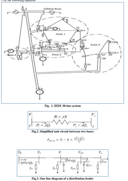
12, 27 and 5 can be selected as the representative load concentration buses of Areas 1 through 4, respectively. When the DG is applied to this system, it is not desirable to connect each DG to every load bus to minimize power loss. Instead, the multiple representative DGs can be connected to the load concentration-buses. Then, they provide an effect similar to the case where there are all DGs on each load bus, but with added benefit of reduced power loss [6]–[9].
The power loss, Plossbetween the two buses i and j is computed from the simplified unit circuit shown
in fig. 2 by the following equation:
Fig. 1. IEEE 30-bus system
Fig.2. Simplified unit circuit between two buses
𝑃𝑙𝑜𝑠𝑠 ,𝑖𝑗 = 𝑃𝑖 − 𝑃𝑗 =
(𝑃𝑖2+ 𝑄𝑖2)𝑟
𝑉𝑖2 (1)
𝑉𝑖+12 = 𝑉𝑖2− 2 𝑟𝑖+1𝑃𝑖+ 𝑥𝑖+1𝑄𝑖 + 𝑟𝑖+12 + 𝑥𝑖+12
𝑃𝑖+12 + 𝑄𝑖2
𝑉𝑖2 (2) Also, the one-line diagram of a distribution feeder with a total of n unit circuits is shown in Fig. 3. When power flows in one of direction, the value of bus voltage, Vi+1, is smaller than that of Vi, and this
associated equation can be expressed by (2). In general, the reactive power, Qi, is reduced by connecting a
capacitorbank on bus i in order to decrease the voltage gap betweenVi+1 and Vi . In other words, the capacitor
bank at bus i makes it possible to reduce power loss and regulate the voltages by adjustingthe value of Qiin
equation(2). If a DG is installed at the location of the capacitor bank, the proper reactive power control of the DG has the same effect on the system as does the capacitor bank. Moreover, the main function of the DG is to supply real supplementary power to the required loads in an effective manner. The variation of power loss is relatively less sensitive to voltage changes when compared to the size of DG. In other words, the amount of real power supplied by the DG strongly influences the minimization of power loss. This means that the DG can control the bus voltage for reactive power compensation independently of its real power control to minimize power loss.
B. Selection of Optimal Location for DGs by Considering Power Loss
Before deriving the equations for the selection of optimal locations of DGs, the following terms are defined.
The factor, D shown in the following is called the generalized generation distribution factor [10]:
Fig.4. Power flow from the k th generator to the other several loads.
Fig.5. Power flow from the several generators to the l th load
Pk: power supplied by the k th generator in a power network
Pl: power consumed by the l th load in a power network
Pk,l: power flowing from the k th generator to the l th load
Fjl,k: power flowing from the k th generator to the l th load through bus j connected to the l th load.
Djl,k: ratio of Fjl,k to the power supplied by the k th generator
Ploss,k: power loss on transmission line due to the power supplied from the k th generator
Fkj,l: power flow from the k th generator to the l th load through bus j connected to the k th generator
Dkj,l: ratio of Fkj,l to the power supplied by the k th generator
Ploss,l: power loss on a transmission line due to power supplied to the l th load
Ploss,ij: power loss between buses i and j
Fig.6. Simplified circuit with only power generations and consumptions
For the first case (case-1), the power supplied from the k th generator to the l th load among several loads is calculated by the following:
𝑃𝑘,𝑙|𝑐𝑎𝑠𝑒 −1= 𝑗𝜖𝑐 (𝑙)𝐹𝑗𝑙 ,𝑘= 𝑗𝜖𝑐 (𝑙)𝐷𝑗𝑙 ,𝑘 𝑃𝑘 (3)
Where c(l) are the buses connected to the l th load. Then, the power loss associated with the k th generator is computed by the following, which is the difference between the power supplied from the k th generator and the sum of powers consumed in loads:
𝑃𝑙𝑜𝑠𝑠 ,𝑘 = 𝑃𝑘− 𝑁𝑙=𝑁𝐺 +1𝑃𝑘,𝑙 (4)
In the same manner, the power supplied from the k th generator among several generators to the l th load is calculated by the following for the second case (case-2):
𝑃𝑘 ,𝑙|𝑐𝑎𝑠𝑒 −2= 𝑗𝜖𝑐 (𝑘)𝐹𝑘𝑗 ,𝑙 = 𝑗𝜖𝑐 (𝑘)𝐷𝑘𝑗 ,𝑙 𝑃𝑙 (5)
Where c(k) are the buses connected to the k th generator. The power loss associated with the l th load is computed by the following:
𝑃𝑙𝑜𝑠𝑠 ,𝑙= 𝑁𝐺𝑘=1𝑃𝑘,𝑙− 𝑃𝑙 (6)
The branch between buses i and j in Fig. 6 can become an arbitrary branch in Fig. 1. This means that the total power loss of the system can be calculated by summing the losses of all branches whenever the DG is connected to any bus. Each loss of the branch is thus simply computed by (1).
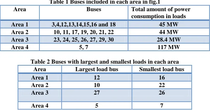
Table 1 Buses included in each area in fig.1
Area Buses Total amount of power
consumption in loads
Area 1 3,4,12,13,14,15,16 and 18 45 MW
Area 2 10, 11, 17, 19, 20, 21, 22 44 MW
Area 3 23, 24, 25, 26, 27, 29, 30 28.4 MW
Area 4 5, 7 117 MW
Table 2 Buses with largest and smallest loads in each area
Area Largest load bus Smallest load bus
Area 1 12 16
Area 2 10 22
Area 3 27 26
Area 4 5 7
3.452 MW will be compared with the total power loss computed after the optimal size of multiple DGs is systematically determined by using the Kalman filter algotihm.
III.
PROCEDURE TO SELECT THE OPTIMAL SIZE OF MULTIPLE DGs USING
KALMAN FILTER ALGORITHM
The total amount of power consumption in Table I at each area could be chosen as the size of DGs to be placed. However, these are not optimal values for the DGs because the power loss in lines connecting two buses is ignored. To deal with this problem, the Kalman filter algorithm is applied to select the optimal sizes of multiple DGs by minimizing the total power loss of system. The Kalman filter algorithm [12], [13] has the smoothing properties and the noise rejection capability robust to the process and measurement noises. In practical environments (in which the states are driven by process noise and observation is made in the presence of measurement noise), the estimation problem for the optimal sizes of multiple DGs can be formulated with a linear time-varying state equation. Also, the error from interval of computation can be reduced during the estimation optimization process. In this study, the state model applied for the estimation is given as
𝑋 𝑛 + 1 = ΦX n + Γω n , x 0 = x0 𝑦 𝑛 = 𝑐 𝑥(𝑛)
𝑧 𝑛 = 𝑦 𝑛 + 𝑣 𝑛 (7)
Where the matrices Φ(ϵ Rn˟n) and Γ(ϵ Rn˟m) and the vector, c(ϵ R1˟n), are known deterministic variables, and the identity matrix I(ϵ Rn˟n) is usually chosen for the matrix Φ. The state vector, x(ϵ Rn˟1) ,, can represent the size of each of the multiple DGs or their coefficients. Also, (ϵ R m˟) is the process noise vector, is the measured power
loss, and v is stationary measurement noise. Then, the estimate of the state vector is updated by using the following steps.
Measurement update: Acquire the measurements, z(n) and compute a posteriori quantities:
𝑘 𝑛 = 𝑃− 𝑛 𝑐𝑇 [𝑐𝑃− 𝑛 𝑐𝑇+ 𝑟]−1
𝑋 𝑛 = 𝑥 − 𝑛 + 𝑘(𝑛)[𝑧 𝑛 − 𝑐𝑥 − 𝑛
𝑃 𝑛 = 𝑃− 𝑛 − 𝑘 𝑛 𝑐𝑃− 𝑛 (8)
Where k(ϵ Rn˟1) is the kalman gain, P is a positive definite symmetric matrix, and r is a positive number selected to avoid a singular matrix 𝑃−(0) is given as 𝑃− 0 = 𝜆𝐼 𝜆 > 0 , where I is an identity matrix.
Time update:
𝑥 − 𝑛 + 1 = Φ𝑥 (𝑛)
𝑃− 𝑛 + 1 = Φ𝑃(𝑛)𝑇+Γ𝑄Γ𝑇 (9)
Where Q(ϵ Rm˟m) is a positive definite covariance which is zero in this study because the stationary process and measurement noises are mutually independent.
Time increment: Increment and repeat.
Thereafter, the estimated output (the total power loss of the system) is calculated as
𝑦 𝑛 = 𝑐 𝑥 𝑛 (10)
In Stage-1 of Fig. 7, the algorithm begins with the zero values for all DGs, and the index denotes the number of given DG. After adding the small amount of power, Pstep of 10 MW to each DG, the initial power loss
is obtained by a power flow computation based on the Newton -Raphson method [5]. Then, the information on the individual power loss, Ploss, corresponding to each DG increased by 10 MW is sent to Stage-2, where the
values of Ploss are substituted with those of Ptemp. After the minimum value of Ptempis selected, its value and the
corresponding sizes of multiple DGs are stored in the memory of Plosses,n and DGi,n in Fig. 7, respectively. This
process is then repeated until the total sum of all DGs is the same as the predefined value, Pmax, in Stage-3 by
increasing n to n+1. Finally, the accumulated data of the minimum power loss and sizes of DGs, which are Plosses,samplesand DGi,samples respectively, are obtained.
application of the Kalman filter algorithm are taken to reduce the error between the estimated and actual values, and then the optimal sizes of multiple DGs are finally estimated.
In Phase-1 of Fig. 8, the estimated sizes of multiple DGs, DGi,estimated, are determined by applying the Kalman
filter algorithm with the data samples obtained from Fig. 7, which are Plosses,samples and DGi,samples. Its associated
parameters are then given in the following:
𝛿 𝑛 = 4𝑖=1𝐷𝐺𝑖,𝑠𝑎𝑚𝑝𝑙𝑒𝑠(𝑛)/max × 4𝑖=1𝐷𝐺𝑖,𝑠𝑎𝑚𝑝𝑙𝑒𝑠(𝑛) (11)
𝑐𝑝ℎ𝑎𝑠𝑒 −1 𝑛 = 𝛿 𝑛 , 𝛿2 𝑛 , 𝛿3 𝑛 , 𝛿4(𝑛) (12) 𝑧 𝑛 𝑖 = 𝐷𝐺𝑖,𝑠𝑎𝑚𝑝𝑙𝑒𝑠(𝑛) (13)
𝐷𝐺𝑖,𝑒𝑠𝑡𝑖𝑚𝑎𝑡𝑒𝑑 𝑛 = 𝑦 𝑛 = 𝑐𝑝ℎ𝑎𝑠𝑒 −1 𝑛 . 𝑥 phase1(nmax)|i
(i=1, 2, 3, 4) (14)
Fig.7. Procedure to obtain data samples of the multiple DGs and power loss required before applying the kalman filter algorithm
Where 𝛿 is the normalized value, and nmax is the number of last samples in DGi,samples. To estimate the size of
each DG, the kalman filter algorithm is applied in sequence with different measurements of z in (13).
After estimating the optimal sizes of multiple DGs in Phase-1, the total power loss, Ploss,estimated, is estimated in
Phase-2 of Fig. 8 with the power loss data samples, Ploss,samples. From Fig. 7 and the estimated DG sizes,
DGi,estimated, in phase-1. The associated parameters required to apply the Kalman filter algorithm are given in the
𝛽𝑖 𝑛 = 𝐷𝐺𝑖,𝑒𝑠𝑡𝑖𝑚𝑎𝑡𝑒𝑑 𝑛 𝑖 = 1, 2, 3, 4 (15)
𝑐𝑝ℎ𝑎𝑠𝑒 −2 𝑛 = 𝛽1 𝑛 , 𝛽2 𝑛 , 𝛽3, 𝑛 , 𝛽4 𝑛 (16)
𝑧 𝑛 = 𝑃𝑙𝑜𝑠𝑠 ,𝑠𝑎𝑚𝑝𝑙𝑒𝑠 𝑛 (17)
𝑃𝑙𝑜𝑠𝑠 ,𝑒𝑠𝑡𝑖𝑚𝑎𝑡𝑒𝑑 𝑛 = 𝑦 𝑛 = 𝑐𝑝ℎ𝑎𝑠𝑒 −2 𝑛 . 𝑥 phase-2(nmax) (18)
Where 𝛽 is the estimated size for each DG from (14).
Fig.8. Steps to estimate the optimal size of multiple DGs in two phases by applying the kalman filter algorithm.
IV.
SIMULATION RESULTS
A. Finding Actual Values
Actual values for each DG and total power loss are required to verify whether the optimal sizes of multiple DGs estimated by the Kalman filter algorithm are acceptable. These values are obtained by taking the following steps.
1) Take the steps in Figs. 7 and 8.
2) Reduce the value of Pstep by half. Note that its initial value used in the previous section is 10MW
3) Repeat step 1) until the state vector, x , in (7) of the Kalman filter algorithm converges to a constant value. 4) Obtain the total n number of actual power losses, 𝑃𝑙𝑜𝑠𝑠 ,𝑠𝑎𝑚𝑝𝑙𝑒𝑠𝑎𝑐 𝑡𝑢𝑎𝑙 , and actual sizes of each DG,𝐷𝐺𝑖,𝑠𝑎𝑚𝑝𝑙𝑒𝑠𝑎𝑐𝑡𝑢𝑎𝑙 .
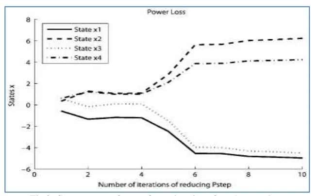
The variations of the state vector, x, at each iteration for the estimation of multiple DGs’ size (in Phase-1 in Fig. 8) and total power loss (in Phase-2 in Fig. 8) are shown in Figs. 9 and Phase-10, respectively.
It is observed that each state converges sufficiently at the tenth iteration according to the above steps. At this time, the value of Pstep is about 0.0195 MW (=10˟(1/2)9). Therefore the actual values,
𝑃𝑙𝑜𝑠𝑠 ,𝑠𝑎𝑚𝑝𝑙𝑒𝑠𝑎𝑐𝑡𝑢𝑎𝑙 𝑎𝑛𝑑 𝐷𝐺𝑖,𝑠𝑎𝑚𝑝𝑙𝑒𝑠𝑎𝑐𝑡𝑢𝑎𝑙 , obtained with the Pstep of 0.0195 MW are reasonably acceptable, and used to
Fig.9. Convergence of states for estimation of total power loss
B. Evaluation of Estimation Performance
To evaluate the estimation performance of the Kalman filter algorithm, the root-mean square error (RMSE) in (19) is computed with actual measurements. The RMSE uses the absolute deviation between the estimated and actual quantities. Due to squaring, it gives more weight to large errors than smaller ones as follows:
RMSE = 1
𝑛 (𝑦𝑚
𝑎𝑐𝑡𝑢𝑎𝑙 − 𝑦
𝑚𝑒𝑠𝑡𝑖𝑚𝑎𝑡𝑒𝑑)2 𝑛−1
𝑚 =0 (19)
Table 3 Comparison of RMSE values
RMSE Sampled Estimated
DG1 2.4662 1.4061
DG2 2.8893 1.6863
DG3 2.9184 1.6363
DG4 3.2082 2.0435
Where n represents the number of data samples. After applying the Kalman filter algorithm, the estimation results for sizes of each DG are shown in Table 3. When compared to the case with data sampled by the Pstep of 10 MW, the estimated sizes of each DG are much more similar to their actual values with smooth
behaviors.
The estimation results for total power loss are also shown in Fig. 10 and Table 5. It is clearly observed that the Kalman filter algorithm provides a very accurate estimation performance when compared to the other sampled case. Correspondingly, the RMSE value of the estimated power loss is very low.
C. Effect by optimal size of multiple DGs
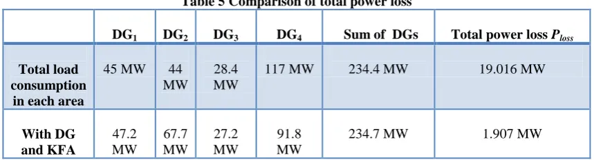
From the result in fig. 10, the minimum value of total power loss is 1.907MW. The corresponding optimal sizes of multiple DGs , which are estimated by the kalman filter algorithm , are 47.2,67.7,27.7,and 91.8MW for the DG1,DG2,DG3and DG4 respectively as shown in Table 5. The summation of the size of all DGs is 234.4MW.
Table 4 Comparison of RMSE values
Power loss Sampled Estimated
Fig.10. Estimation performance of total power loss
When the initial values of multiple DGs are used, the corresponding total power loss is 3.452MW even though the summation of the initial size of all DGs is same as the above case with 234.4MW.
Table 5 Comparison of total power loss
DG1 DG2 DG3 DG4
Sum of DGs Total power loss Ploss
Total load consumption
in each area
45 MW 44 MW
28.4 MW
117 MW 234.4 MW 19.016 MW
With DG and KFA
47.2 MW
67.7 MW
27.2 MW
91.8 MW
234.7 MW 1.907 MW
Finally, the total power loss is effectively reduced by the optimal size selection process. In particular, note that the size in Area 2 is required to increase from 44 to 67.7 MW, of which is a difference of 23.7 MW. In contrast, the size of in Area 4 is necessary to decrease significantly from 117 to 91.8 MW, which is difference of 25.2 MW.
V.
COST ANALYSIS
A power system can usually be divided into the subsystems of generation, transmission, and distribution facilities according to their functions. The basic function of the electrical power system is to supply the electricity to consumers with reliability and quality. Basically the consumers are far away from the generating stations, so they are severely effected by the low voltages. In order to improve the voltage levels we can generate the power locally by using the distributed generation(DG). Based upon distributed generation, we can also estimate the cost of generation.
The annual cost ($) due to the power loss is calculated by
𝐶𝑡 = 𝑃𝑙𝑜𝑠𝑠 ,𝑋. 𝐹𝑙𝑜𝑠𝑠. 𝐾𝐸. 8760 (20)
Where KE is the energy cost ($/kWh) and Floss is the power loss factor which is the ratio between the average
power loss and the peak power loss and is given as
KE = 12.2600$/kWh (21)
𝐹𝑙𝑜𝑠𝑠 =
𝐴𝑣𝑒𝑟𝑎𝑔𝑒 𝑝𝑜𝑤𝑒𝑟 𝑙𝑜𝑠𝑠
To compute Floss , a segment of historical load profile over a certain period is obtained from the
metering database, and the power loss at each time point is calculated by running power flow. The peak power loss is the power loss at the peak load point and the average power loss is the average value of all of the time.
Table 6 Cost analysis
Without DG and KFA With DG and KFA
Cost of generation( $) 178508.328 25827.018
Profit( $) - 152681.310
VI.
CONCLUSION
This paper proposed the method for selecting the optimal locations and sizes of multiple distributed generations (DGs) to minimize the total power loss and cost generation. To deal with this optimization problem, the Kalman filter algorithm was applied. When the optimal sizes of multiple DGs are selected, the computation efforts might be significantly increased with many data samples from a large-scale power system because the entire system must be analyzed for each data sample. The proposed procedure based on the Kalman filter algorithm took the only few samples, and therefore reduced the computational requirement dramatically during the optimization process.
Prior to the implementation and connection to an electric power grid, this study can be used as a decision-making process in the power system operation and planning for selecting the optimal locations and sizes of multiple DGs based on the renewable energy resources such as fuel cell, photovoltaic, micro-turbines, wind powers, etc.
REFERENCES
[1]. A. A. Chowdhury, S. K. Agarwal, and D. O. Koval, “Reliability modeling of distributed generation in conventional distribution systems planning and analysis,” IEEE Trans. Ind. bAppl., vol. 39, no. 5, pp.1493–1498, Oct. 2003.
[2]. M. F. AlHajri and M. E. El-Hawary, “Improving the voltage profiles of distribution networks using multiple distribution generation sources,” in Proc. IEEE Large Engineering Systems Conf. Power Engineering, 2007, pp. 295–299.
[3]. G. Carpinelli, G. Celli, S. Mocci, F. Pilo, and A. Russo, “Optimization of embedded eneration sizing and siting by using a double trade-off method,” Proc. Inst. Elect. Eng. Gen., Transm., Distrib., vol. 152, no.4, pp. 503–513, Jul. 2005
[4]. T. Senjyu, Y. Miyazato, A. Yona, N. Urasaki, and T. Funabashi, “Optimal distribution voltage control and coordination with distributed generation,”
[5]. IEEE Trans. Power Del.,vol. 23, no. 2, pp. 1236–1242, Apr. 2008.
[6]. H. Saadat, Power System Analysis, 2nd ed. , Singapore: McGraw- Hill, 2004, pp. 234– 227.
[7]. J. J. Grainger and S. H. Lee, “Optimum size and location of shunt capacitors for reduction of losses on distribution feeders,” IEEE Trans. Power App. Syst., vol. PAS-100, no. 3, pp.1105–1118, Mar. 1981. [8]. M. Baran and F. F. Wu, “Optimal sizing of capacitors placed on a radial distribution system,” IEEE
Trans. Power Del., vol. 4, no. 1, pp. 735–743, Jan. 1989.
[9]. M. A. Kashem, A. D. T. Le, M. Negnevitsky, and G.Ledwich, “Distributed generation for minimization of power losses in distribution systems,” in Proc. IEEE PES General Meeting, 2006, pp. 1–8.
[10]. H. Chen, J. Chen, D. Shi, and X. Duan, “Power flow study and voltage stability analysis for distribution systems with distributed generation,” in Proc. IEEE PES General Meeting, Jun. 2006, pp. 1–8.
[11]. W. Y. Ng, “Generalized generation distribution factors for power system security evaluations,” IEEE Trans. Power App. Syst., vol. PAS-100, no. 3, pp. 1001–1005, Mar.1981
[12]. Y.-C. Chang and C.-N. Lu, “Bus-oriented transmission loss allocation,” Proc. Inst.Elect. Eng., Gen., Transm., Distrib., vol. 149, no. 4, pp. 402–406, Jul. 2002.
[13]. R. A. Wiltshire, G. Ledwich, and P. O’Shea, “A Kalman filtering approach to rapidly detecting modal changes in power systems,” IEEE Trans. Power Syst., vol. 22, no. 4, pp.1698–1706, Nov. 2007. [14]. E. W. Kamen and J. K. Su, Introduction to Optimal Estimation. London, U.K.: Springer- Verlag, 1999,
pp. 149–183.