R E S E A R C H
Open Access
A robust iterative algorithm for image
restoration
Yuewei Liu
1,2and Weiping Lu
2*Abstract
We present a new image restoration method by combining iterative VanCittert algorithm with noise reduction modeling. Our approach enables decoupling between deblurring and denoising during the restoration process, so allows any well-established noise reduction operator to be implemented in our model, independent of the VanCittert deblurring operation. Such an approach has led to an analytic expression for error estimation of the restored images in our method as well as simple parameter setting for real applications, both of which are hard to attain in many regularization-based methods. Numerical experiments show that our method can achieve good balance between structure recovery and noise reduction, and perform close to the level of the state of the art method and favorably compared to many other methods.
Keywords: Image restoration, Ill-posed problem, Iterative cost function, Regularized gradient, Noise reduction filter, Residual optimization
1 Introduction
Image restoration aims to compensate for or undo the defects that degrade an image. Degradation can come in many forms such as motion blur, noise, and camera defo-cus. In optical microscopes, there are predominately two sources for degradation in the imaging systems, blurring and noise, which can be described by the general imaging model
J=PI+N, (1)
where I,J are the ground truth and the corresponding observation, respectively, P is a point spread function (PSF), andN is a noise which is assumed to be indepen-dent to the ground truth. The simplest way to estimate the ground truth from the observation is by minimizing the residual,
minJ−PI22, (2)
which can lead to the least square solution. Unfortunately, a unbounded noise will be introduced into the solution because the PSF matrix always has small eigenvalues even
*Correspondence: [email protected]
2School of Engineering and Physical Sciences, Heriot Watt University, Edinburgh, UK
Full list of author information is available at the end of the article
it is invertible. This is not surprising as (2) is well known to be ill-posed [1].
There are now vast literatures to tackle the problem of image restoration. A recent trend is concentrated on a sparse block matching 3-D (BM3D)-based restoration technique. BM3D algorithms are initially developed for collaborative filtering through a non-local modeling of images by collecting similar image patches in 3D arrays [2]. They have recently been incorporated into image restoration for solving regularized inverse problems for image denoising as well as deblurring [3]. Another devel-opment based on BM3D is sparse representation for image restoration, where the image is considered to be a combination of a few atomic functions taken from a certain dictionary and can be parameterized and approx-imated locally or non-locally by these functions [4]. The dictionary is usually considered as an over-complete sys-tem in order to better describe all variety of images. There are now many published works on the sparsity-based models and methods [5]. For example, the formulation of IDD-BM3D image modeling in terms of the over-complete sparse frame representation for image recon-struction has led to impressive restoration performance [6]. This approach allows decoupling between deblurring and denoising by considering the optimization problem
as a generalized Nash equilibrium balance of two objec-tive functions. A distinct advantage of this approach is that various denoising algorithms can be selected inde-pendently with respect to deblurring algorithms, which have demonstrated better performance than those where deblurring and denoising are jointly performed in many cases. However, for the decoupled algorithms such as [6], [7], and [8], the parameters setting for optimal perfor-mance of regularization is usually complicated and rea-sons for the best setting are often not explained. Another shortage of these methods is the lack of error analysis for the solutions because of the complexity of the regulariza-tion factors.
In this paper, we present a new image restoration method based on the inverse operator theory. As we know, the inverse operator theory [9] gives the solution of P−1J=I+P−1Nfor the general imaging model (1), where P−1is the inverse or pseudo-inverse of the PSF matrix. Due to small eigenvalues ofP,P−1N leads to significant noise amplification to the ground truth. To overcome this problem, we propose a new approach that combines itera-tive VanCittert algorithm with noise reduction modeling, the latter enables to reliably estimate the gradient in the presence of noise so that the VanCittert iteration can con-verge to the ground truth even when the observation is noise contaminated. This work has several contributions to the research area of image restoration. Firstly, it extends the inverse operator theory to image restoration in the presence of noise, which offers a different approach to that of the present popular regularization methods. Secondly, our method enables decoupling between deblurring and denoising, so any well-established noise reduction oper-ator can be selected in our model, independent of the VanCittert deblurring operation. Thirdly, our approach allows error analysis of the solutions because the structure recovery and noise amplification in the VanCittert itera-tions can be separated analytically, which is an advantage over many regularization methods for which errors are difficult to be estimated due to complicated regularization factors. Finally, parameter setting in our method is simple and robust to the performance. There are only two param-eters in our method:σ, as the noise reduction strength, and s, the interval between two neighboring denoising operations. We have further developed an automated parameter setting procedure for our method, which has no need to set the parameters manually. The above points have been verified by numerical experiments, which also show that our method performs close to the level of the state of the art method and favorably compared to many other methods.
2 Methods
Our method is motivated by the iterative VanCittert algo-rithm, which has a long history as a simple and efficient
approach for image restoration. The algorithm is formu-lated for spatially invariant or variant restoration prob-lems with neglect of noise contribution in (1). Originally, it is a steepest descent method but the solution does not converge if the step parameter is assumed to be real val-ues. To overcome this shortage, an iterative procedure was proposed [10],
Ik=Ik−1+βPT(J−PIk−1), (3) which converges to the ground truth only if noise in an observation is negligible, where PT is the transpose
of P. When an observation comprises noise, VanCittert iteration (3) can be expressed as [9, 11, 12]
Ik=
u,v
1−1−β|ζuv|2
k
(I,Zuv)Zuv
+
u,v
1
ζuv
1−1−β|ζuv|2
k
(N,Zuv)Zuv
fork=1, 2,. . ., (4)
where {ζuv : u = 1, 2. . .,R,v = 1, 2,. . .,C} and Zuv
are the eigenvalues and eigenvectors of P, andR, C are image size, andu,vthe indices of image pixels andβ the step parameter. The first term involvingIdescribes struc-ture recovery while the second term involvingN shows noise amplification, so structures and noise are separated in (4). For a noisy observation, however, small eigenvalues
ζuvcan lead to significant noise amplification in the
sec-ond term of (4) so the inverse problem becomes ill-posed. Therefore, we have to suppress the noise in the second term if the iteration gives any hope to converge to the ground truth.
To tackle the above problem, we first introduce a noise reduction operator, , which minimizes the estimation error of a cost function. Letting I be the ground truth, N be a white noise and V = I+N, we define the cost function for the noise reduction operator,
C(,I)=EI−(V)22,
where E{·}is the expectation taken over the noise distri-bution. The error is measured byL2norm and averaged over the noise distribution. For the general imaging model (1), we propose our method as
⎧ ⎪ ⎨ ⎪ ⎩
Ik =Ik−1+βPT(J−PIk−1) (5a) RN =arg min
C(,Dk), (5b)
Ik =RN(Ik), fork=1, 2,. . ., (5c)
whereDk = u,v
1−1−β|ζuv|2
k(
I,Zuv)Zuv, is the
and (5c) is then applied to remove noise and to optimize the gradient for the next iteration.
As for noise reduction of (5b), our method do not expect an ideal operator removing all noise [13]. Instead, it can be any denoising algorithm as long as the operator satisfies the following condition,
RN(I+N)=I+o(N)and Var(o(N))∝σ2, (6)
whereσ2=Var(N)is the variances of noiseNand1 is the noise reduction factor. The condition (6) implies that remaining noiseo(N)has a variance far less than the initial noiseNafter applying the operatorRN on a noisy
image. We will show in error analysis below that when the condition (6) is satisfied, the iterative solution of (5) con-verges to the ground truth with a higher order small noise term, i.e.,Ik→∞=I+o(N). A necessary condition for the
iterative process (5) to converge is that|1−β|ζuv|2|must
fall within [ 0, 1)for all the eigenvalues ofP, which leads to
0< β≤minu,v
2
|ζuv|2
. (7)
Since most of PSFs act as a low-pass filter, the maximum absolute value of their eigenvalues is about 1. This means that it is easy to set a value forβthat satisfies condition (7) and the following condition:
0≤(1−β|ζuv|2) <1for all the eigenvalues. (8)
For example, we setβ=1 in our experiments.
To implement the method (5), we can apply any well-established noise reduction algorithms to combine with the VanCittert iteration, for example, the wavelet domain shrinking filter TSW(V,δ) = ˆI = Ww, where ˆI is the
estimated image, W is a group of wavelet bases and w is a vector of shrinking coefficients depending on the smooth parameterδ[13]. The smooth parameterδcan be determined in a similar form to (5b) by
arg min
δ C(TSW(V,δ),I),
which has a noise shrinkage strength of= (2logRC+ 1)(logRC+ 1)/RC, where R and C are the image size. For images of modest size, 1 so the wavelet algo-rithm satisfies (6). Another popular denoising method is the state of the art BM3D method. BM3D improves from wavelet domain shrinking by incorporating the con-cept of image patches and non-local mean (NLM) [14] into a transformed domain and has shown the highest peak signal-to-noise ratio in its performance compared to the wavelet domain and other algorithms. Moreover, BM3D has simple parameter setting and is easy to use. Mathematically, BM3D can be expressed as
OBM3D=AT3D−1WwieT3DZ, (9)
whereZ is the stacked noisy blocks,T3Dis the transfor-mation from spatial domain to frequency domain with
discrete cosine bases, andWwie is the Wiener shrinkage operator andAis the aggregation operator, all defined in [2]. In view of the advantage and excellent performance of BM3D [2], we choose the operatorRN = OBM3D in our method (5) for the numerical experiments below.
We note that while we follow the same decoupled approach for deblurring and denoising as IDD-BM3D [6], our method has two advantages. Firstly, structure restora-tion by the VanCittert algorithm in (5) has a simple step parameter ofβ = 1, while the regularization factors for optimal deblurring in [6] and [7] are much more complex to set. This leads to overall simple parameter setting of our method compared to many regularization methods. Secondly, structure and noise can be separated analyti-cally in (5), which allows us to perform error analysis for a restored image, while error analysis for regularization methods is generally hard to attain due to the complexity of the regularization factors.
2.1 Error analysis
Given (4), the noise amplification is separated from struc-tures so VanCittert algorithm allows error analysis for our method. We begin with the following lemma and then give theorem (1).
Lemma 1Let Fk = 1/ζuv
1−1−β|ζuv|2
k
be the noise amplification factor in Eq.(4), then1≤Fk/Fk−1<2 forβsatisfying(8)and k≥2.
ProofFor convenience we set a = (1−β|ζuv|2), thus
Fk = 1/ζuv(1−ak). Because of condition (8)adrops in
[ 0, 1). The ratio
Fk Fk−1 =
1−ak
1−ak−1 =
1+a+a2+ · · · +ak−1 1+a+a2+ · · · +ak−2
=1+ a
k−1
1+a+a2+ · · · +ak−2, so 1≤Fk/Fk−1<2 for anya∈[ 0, 1)whenk≥2.
Theorem 1For any operator RNsatisfying condition(6)
and β satisfying (8), the iterative solution of model (5) leads to
lim
k→∞Ik=I+o(N), (10)
ProofLetFk = 1/ζuv(1−(1−β|ζuv|2)k)be the noise
amplification factors fork=1, 2. . .. Known from lemma (1),Fk is infinite so there must be a minimum numberk
satisfying
Var
u,v
N Fk
,Zuv
Zuv
<Var(N) (11)
when noiseN is bounded. Here, we suppose k = 1 for convenience though this number depends the eigenval-ues ofP. Thus, we start with the iteration solution(4) for k=1,
I1=I0+βPT(J−PI0)
=
u,v
1−1−β|ζuv|2
(I,Zuv)Zuv
+
u,v
1
ζuv
1−1−β|ζuv|2
(N,Zuv)Zuv
=D1+N1, (12)
whereI0is the initial image andD1is the first sum on right side. The first term in (12) is noise-free iterative solution while the second term is noise contribution with the factor F1 = βζuv. Since most of the eigenvalues have absolute
values small than 1, Var(N1)∝Var(N). Then we apply the filter (6) to (12) and have
I1=RN(I1)=RN(D1+N1)=D1+o(N1). (13)
The noise is now reduced by a factor 1 according to (6), i.e., Var(o(N1)) ∝ Var(N1) ∝ σ2, whereσ2is the variance of noiseN.
The intensity of imageI1can be rewritten
I1=D1+o(N1)
=
u,v
1−1−β|ζuv|2(I,Zuv)Zuv
+
u,v
1
ζuv
1−1−β|ζuv|2
o(N1) F1
,Zuv
Zuv,
(14)
whereo(N1)=uv(o(N1),Zuv)Zuv=uvF1(o(N1)/F1, Zuv)Zuv is used andF1is defined at the beginning of the proof.
From (14) and (4), we give the iteration solution for k=2
I2=I1+βPT(J−PI1)
=I1+βPT
PI+
u,v
o(N1)
F1 ,Zuv
Zuv−n1
+βPT
N−
u,v
o(N1)
F1 ,Zuv
Zuv
=
u,v
1−1−β|ζuv|2
2
(I,Zuv)Zuv
+
u,v
1
ζuv
1−1−β|ζuv|2
2 o(N1) F1
,Zuv
Zuv
+βPT
N−
u,v
o(N1)
F1 ,Zuv
Zuv
=D2+
u,v
F2 F1(
o(N1),Zuv)Zuv
+βPT
N−
u,v
o(N1)
F1 ,Zuv
Zuv
=D2+N2.
whereN2is the sum of the two noise terms on the right side. By (11) and lemma (1), 1 ≤ F2/F1 < 2, Var(N2) ∝ Var(N)=σ2is obtained.
Repeating in the operation (13) we have
I2=RN(I2)=RN(D2+N2)=D2+o(N2),
where the variance ofo(N2)is far less than that ofN2, also far less than that ofN.
In general, we have
Ik=Dk+Nk,
where
Dk=
u,v
1−1−β|ζuv|2k
(I,Zuv)Zuv
and
Nk=
uv
Fk
Fk−1
oNk−1,Zuv
Zuv
+βPT
N−
uv
o(Nk−1) Fk−1
,Zuv
Zuv
.
By applyingRNtoIk, we get the iterative image
Ik=RN(Ik)=Dk+o(Nk),
where Var(o(Nk)) ∝ Var(N) = σ2. Therefore, the
Table 1PSF and noise variation for each scenario
Scenario Blur PSF σ2
1 1/(1+x2+y2),x,y= −7,. . ., 7 2
2 1/(1+x2+y2),x,y= −7,. . ., 7 8
3 9×9 uniform 0.3
4 [ 1 4 6 4 1]T[ 1 4 6 4 1]/256 49
5 Gaussian with std=1.6 4
6 Gaussian with std=0.4 64
noise is controlled to the order of σ2 in the iterative process.
It can be seen from the above derivation that the sep-aration of structure recovery from noise amplification in the VanCittert expression is the key that enables us to express noise amplification factor in thekth iteration to beFk/Fk−1, which is always between 1 and 2 for allk. This makes it possible to control the noise amplification over a finite number of iterations by a noise reduction operator satisfying (6). Consequently, the iterative solution con-verge to the ground truth with higher-order infinitesimal noise.
3 Results and discussion
In this section, we undertake two experiments to test our method and compare the results with existing meth-ods. The first experiment contains two images, ’Cam-eraman256.png’ and ’Lena512.tif ’, that are commonly used for measuring efficiency of algorithms for struc-ture restoration because they contain elaborate strucstruc-tures,
such as lines, buttons, and textures. These images are the subjects of a recent extensive investigation by an itera-tive decoupled deblurring BM3D algorithm (IDD-BM3D) [6], which is formulated based on the Nash equilibrium balance of two objective functions undertaking sepa-rate denoising and deblurring operations. IDD-BM3D has showed state of the art restoration performance com-pared to seven other existing methods, which include Fourier-Wavelet regularized deconvolution (ForWaRD) [15], space-variant Gaussian scale mixtures (SV-GCM) [16], shape-adaptive discrete cosine transform(SA-DCT) [17], BM3D deblurring (BM3DDEB) [3], analysis-based sparsity (L0-Abs) [18], adaptive total variation image deblurring by a majorization minimization approach (TVMM) [19], and finally a method based on spatially weighted total variation (CGMK) [20]. We test on the same six scenarios in [6], which have different PSF shapes and blurring strengths as well as noise levels listed in Table 1. Comparisons with all the eight methods are made quantitatively through the measurement of peak signal-to-noise ratio (PSNR).
As discussed earlier, we choose BM3D (http://www. cs.tut.fi/~foi/GCF-BM3D) as our noise reduction filter because it combines the transform-domain filter [13] with non-local mean filter [14] and has shown improved per-formance over the both methods individually on their own. Our method is easy to operate, requiring only two parameters: noise standard deviation,σ, as an input for BM3D denoising and the step interval, s, between two neighboring denoising operations in the iteration (denois-ing is not necessary for each iteration step for efficient computing). In general, the two parameters depend on the levels of blur and noise in an observation (input
Table 2PSNR of the methods in six scenarios
Scenarios Scenarios
1 2 3 4 5 6 1 2 3 4 5 6
Methods Cameraman (256×256) Lena (512×512)
Input PSNR 22.23 22.16 20.76 24.62 23.36 29.82 25.61 25.46 24.11 28.06 27.81 29.98
ForWaRD [15] 28.99 27.24 28.10 27.02 26.50 33.74 33.30 31.94 32.81 31.74 32.66 35.45
SV-GSM [16] 29.68 27.71 28.09 27.35 26.61 34.01 - - -
-SA-DCT [17] 30.34 28.49 29.31 27.99 27.08 34.53 34.8 33.14 33.63 33.3 33.24 35.87
BM3DDEB [3] 30.42 28.56 29.1 27.96 27.09 34.52 35.2 33.57 33.81 33.62 33.53 36.43
L0-Abs [18] 29.93 27.93 29.72 27.61 26.94 33.21 33.91 32.75 33.63 32.9 33.38 31.96
TVMM [19] 29.64 27.33 29.3 27.19 26.72 31.12 33.61 32.02 33.31 32.33 32.77 32.82
CGMK [20] 30.03 27.65 29.91 27.42 26.9 33.15 34.01 32.41 33.7 32.3 33.09 34.49
IDD-BM3D [6] 31.08 29.28 31.21 28.60 27.67 34.71 35.22 33.65 34.75 33.78 34.01 36.37
Ours(BM3D) 30.73 28.71 30.57 28.25 27.43 34.65 35.29 33.41 34.53 33.70 33.91 36.46
Ours(TSW) 28.62 26.52 27.99 26.18 26.04 32.23 33.90 32.38 32.85 32.43 32.87 34.27
Table 3SSIM of the four methods in six scenarios
Scenarios
1 2 3 4 5 6
Methods Cameraman (256×256)
Input SSIM 0.93 0.93 0.92 0.96 0.95 0.98
L0-Abs 0.99 0.98 0.99 0.98 0.98 0.99
BM3DDEB 0.99 0.99 0.99 0.98 0.98 0.99
IDD-BM3D 0.96 0.94 0.95 0.96 0.96 0.99
Ours(BM3D) 0.99 0.99 0.99 0.98 0.98 0.99
Ours(TSW) 0.97 0.97 0.97 0.96 0.96 0.99
The italicized values in this table indicate the method which leads to the best result among all compared methods
image). We have found that our method can produce good performance in a large area in the two parameter space, showing the robustness of the method against the set-ting of the two parameters. The solutions converge around 1200 iterations for all scenarios except scenario 3 which requires 10,000 iterations because of severe blur in this scenario. Due to high noise levels in scenarios 4 and 6, BM3D is applied to the observations before our iterative algorithm is implemented. To investigate the effects of dif-ferent denoising algorithms on the performance of our method, we have also implemented the wavelet domain shrinking filterTSW as an alternative denoising operator in our method. Table 2 shows the results of PSNR for our algorithm, both with BM3D andTSW, and the eight exist-ing methods, the latter are from [6]. From the table, we can conclude that our method with BM3D outperforms the existing seven methods for both images under different
scenarios and is not far behind the state-of-the-art IDD-BM3D. As expected, the algorithm withTSWperforms not as good as that with BM3D, because the latter is better than the former as a denoising method.
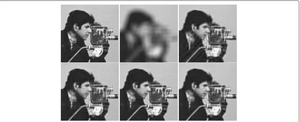
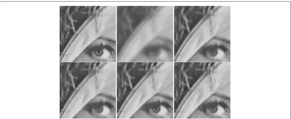
We have further investigated the above results by using the structural similarity (SSIM) index matric, which is a method for measuring the structural similarity between two images. The results are shown in Table 3. As seen from the table, L0-Abs, BM3DDEB, and our methods both with BM3D andTSWhave all performed better than IDD-BM3D in terms of SSIM for the first five scenar-ios, although IDD-BM3D gives the highest PSNR values as discussed above. By comparing the results in Tables 2 and 3, it is pleasing to see that our method with BM3D gives very good and balanced performance in terms of both noise reduction and structure preservation. Figures 1 and 2 show the restored images by four methods used. As seen by visual inspection, BM3DDEB produces some obvious artifacts around the edge of cameraman and L0-Abs cannot restore some details of the eye in the image of Lena because of noise. In comparison, IDD-BM3D and our method with BM3D denoise very well and our method shows better recovery of elaborative features in these images.
We have further developed an automated parameter setting procedure for our method. Here, we first esti-mate the noise standard deviation in the observation and set this value as the denoising threshold, σthr. During
the iteration, the noise level of the image is estimated at each iteration step and when it exceedsσthr, then BM3D denoising is applied. The procedure is simple to operate, which can be important for real scene applications. We
Fig. 2Deblurring of Lena image, scenario 2. Fromlefttorightand fromtoptobottomare presentedzoomedfragments of the following images:
original,blurred, andnoisy, reconstructed by BM3DDEB, L0-Abs, IDD-BM3D, and our method. In our method, the two input parameters used,(σ,s), are(7.5, 25)for this scenario,(7.5, 85)for scenario 1,(7.5, 550)for scenario 3,(7.5, 10)for scenario 4,(7.5, 50)for scenario 5, and(7.5, 5)for scenario 6
used this procedure in the second experiment of Jet-plane.png, and the result are compared with those of IDD-BM3D and the fast non-convex non-smooth method (Fnnmm) method [21] on PSNR and text restorations. Fnnmm introduces non-convex functions applied on dis-crete total variation as a regularization and provides fast algorithms to minimize the energy function. The code of Fnnmm is downloaded at http://www.math.hkbu.hk/~ mng/imaging-software.html. We used the same six sce-narios as in the first experiment, which in turn allows us to use the same parameter setting for IDD-BM3D. For Fnnmm, we fix parameter αep to be 0.5 as given in the
paper and scan the other parameter for each of the six sce-narios for the highest possible value of PSNR. The PSNR values of restored images are given in Table 4. As seen in the table, our method with automated parameter setting, IDD-BM3D and our method with fixed parameter setting
Table 4PSNR of the three methods in six scenarios
Scenarios
1 2 3 4 5 6
Methods Jetplane (512×512)
Input PSNR 24.98 24.84 23.43 27.31 26.84 29.85
Fnnmm [21] 33.10 30.89 32.97 30.76 30.60 34.91
IDD-BM3D [6] 35.43 33.41 34.58 32.63 32.12 36.60
Ours (fixed parameters) 35.03 32.84 34.57 32.91 32.04 36.65
Ours (automated parameters)35.44 33.34 34.29 33.35 32.42 36.27
The italicized values in this table indicate the method which leads to the best result among all compared methods
achieved 3, 2, and 1 best values out of the 6 scenarios, respectively, but differences among them are small and all of them are significantly better than those of Fnnmm. Figure 3 shows a zoomed area of the body of the plane. Our results show slightly better resolution on some of the letters on the plane.
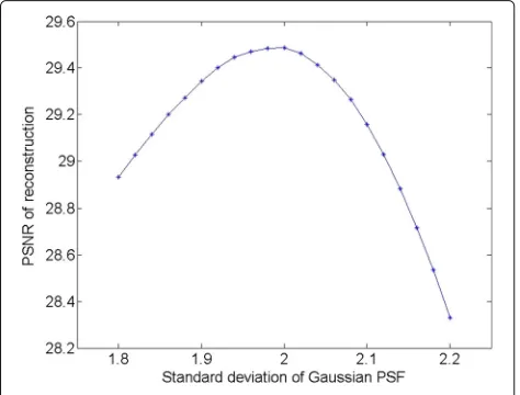
Finally, we test the robustness of our method against the fluctuations of the size of PSF in the model, since the exact value is usually unknown in practice and is estimated. For this, we undertake the experiment on image Jetplane.png, which is blurred by a Gaussian PSF of standard deviation
σ = 2 and noise level of 40 db. We measure PSNR of the restored images on varyingσ by±10% from the exact value. As shown in Fig. 4, PSNR decreases from its peak value of 29.5 on both sides, dropping faster when σ is larger, due to more noticeable artifacts of the hard shoul-der and plunge effects around an edge in this situation. As a result, the restored image looks to artificially have a higher contrast whenσ is larger than the exact value. Overall, the reduction of PSNR is 2 and 4% by varying the standard deviation 10% smaller or larger than the exact value, respectively.
4 Conclusions
Fig. 3Deblurring of Jetplane image, scenario 5. Fromlefttorightand fromtoptobottomare the following images:blurredandnoisy, fragments of
original,blurred,andnoisy, results of Fnnmm, IDD-BM3D, and ours. In our method (fixed parameters), the two input parameters,(σ,s), are(7.5, 50) for this scenario,(7.5, 85)for scenario 1,(7.5, 25)for scenario 2 ,(7.5, 550)for scenario 3,(7.5, 10) for scenario 4, and(7.5, 5)for scenario 6. In our method with automated parameter setting,σthr=3
by an order of magnitude smaller than the noise level in the observation. Different from the well-established reg-ularization methods, which introduce a penalty to solve the ill-posed problem, we directly apply VanCittert algo-rithm to minimize residual along gradient for structure restoration and to suppress noise through a noise reduc-tion operator. It turns out to be a denoising problem in an iterative manner, and the noise can be removed judiciously by applying existing noise reduction methods. We have undertaken two numerical experiments to investigate the performance of this method and compare to existing reg-ularization methods. We show that our method performs
Fig. 4PSNR of reconstruction with different PSFs
to the level close to the best of the methods currently available in terms of recovering elaborate structures and reducing noise, and favorably compared to the many other existing methods. Moreover, our method requires simple parameter setting, particularly in the second experiment where a single parameter is estimated from the obser-vation. This could be a great advantage for real-world applications. We note finally that we have only considered additive noise in this paper, for images contaminated by multiplicative noise, some newly developed noise reduc-tion filters, such as [22] may be applied, which can be our future work in this area.
Abbreviations
BM3D: Block matching 3-D; CGMK: Chantas, Galatsanos, Molina, Katasaggelos; Fnnmm: Fast non-convex non-smooth method; ForWaRD: Fourier-wavelet regularized deconvolution; IDD-BM3D: Iterative decoupled deblurring block matching 3-D; L0-Abs:L0Analysis-based sparsity; NLM: Non-local mean; PSF:
Point spread function; PSNR: Peak signal-to-noise ratio; SA-DCT:
Shape-adaptive discrete cosine transform; SV-GCM: Space-variant Gaussian scale mixtures; TVMK: Total variation image deblurring by a majorization minimization
Funding
This work is partially supported by the Engineering and Physical Sciences Research Council (UK), project number: EP/K503915/1.
Availability of data and materials
The web links to the sources of the data ( namely, images) used for our experiments and comparisons in this work have been provided in this article.
Authors’ contributions
Competing interests
The authors declare that there are no competing interests.
Publisher’s Note
Springer Nature remains neutral with regard to jurisdictional claims in published maps and institutional affiliations.
Author details
1School of Mathematics and Statistics, Lanzhou University, Lanzhou, China. 2School of Engineering and Physical Sciences, Heriot Watt University,
Edinburgh, UK.
Received: 16 December 2016 Accepted: 20 July 2017
References
1. AN Tikhonov, VY Arsenin,Solutions of ill-posed problems. (Winston, Washington, 1977), pp. 7–25
2. K Dabov, A Foi, V Katkovnik, K Egiazarian, Image denoising by sparse 3-d transform-domain collaborative filtering. IEEE Trans. Image Process.16(8), 2080–2095 (2007)
3. K Dabov, A Foi, V Katkovnik, K Egiazarian,A nonlocal and shape-adaptive transform-domain collaborative filtering,Paper presented in Proceedings of International Workshop on Local and Non-Local Approximation in Image Processing (LNLA), (Lausanne, 2008)
4. O Christensen,An introduction to frames and Riesz bases. (Birkhüser, Boston, 2003)
5. M Elad,Sparse and redundant representation: from theory to application in signal and image processing. (Springer, New York, 2010)
6. A Danielyan, V Katkovnik, K Egiazarian, Bm3d frames and variational image deblurring. IEEE Trans. Image Process.21(4), 1715–1728 (2012) 7. YW Wen, MK Ng, WK Ching, Iterative algorithms based on decoupling of
deblurring and denoising for image restoration. SIAM J. Sci. Comput.
30(5), 2655–2674 (2007)
8. LJ Deng, H Guo, TZ Huang, A fast image recovery algorithm based on splitting deblurring and denoising. J. Comput. Appl. Math.287, 88–97 (2015)
9. RL Lagendijk, J Biemond,Iterative identification and restoration of images. (Springer, Boston, 1991)
10. S Kawata, Y Ichioka, Iterative image restoration for linearly degraded images II.Reblurring procedure. J. Opt. Soc. Am.70(7), 762–772 (1980) 11. MZ Nashed,Aspects of generalized inverses in analysis and regularization,
Generalized inverses and applications. (Academic Press, New York, 2014), pp. 193–244
12. M Nashed, Operator-theoretic and computational approaches to ill-posed problems with applications to antenna theory. IEEE Trans. Antennas Propag.29(2), 220–231 (1981)
13. DL Donoho, JM Johnstone, Ideal spatial adaptation by wavelet shrinkage. Biometrica.81(3), 425–455 (1994)
14. A Buades, B Coll, JM Morel, A review of image denoising algorithms, with a New One. Siam J. Multiscale Model. Simul.4(2), 490–530 (2005) 15. R Neelamani, H Choi, R Baraniuk, Forward: Fourier-wavelet regularized
deconvolution for ill-conditioned systems. IEEE Trans. Signal Proc.52(2), 418–433 (2004)
16. J Guerrero-Colón, L Mancera, J Portilla, et al., Image restoration using space-variant gaussian scale mixtures in overcomplete pyramids. IEEE Trans. Image Process.17(1), 27–41 (2008)
17. A Foi, K Dabov, V Katkovnik, K Egiazarian,Shape-adaptive dct for denoising and image reconstruction.Paper presented in Electronic Imaging, International Society for Optics and Photonics, (San Jose, 2006), pp. 60640N–60640N
18. J Portilla,Image restoration through l0 analysis-based sparse optimization in tight frames.Paper presented in 16th IEEE International Conference on Image Processing (ICIP). (IEEE, Cairo, 2009), pp. 3909–3912
19. JP Oliveira, JM Bioucas-Dias, MA Figueiredo, Adaptive total variation image deblurring: a majorization–minimization approach. Signal Process.
89(9), 1683–1693 (2009)
20. G Chantas, NP Galatsanos, R Molina, AK Katsaggelos, Variational bayesian image restoration with a product of spatially weighted total variation image priors. IEEE Trans. Image Process.19(2), 351–362 (2010)
21. M Nikolova, MK Ng, C-P Tam, Fast nonconvex nonsmooth minimization methods for image restoration and reconstruction. IEEE Trans. Image Process.19(12), 3073–3088 (2010)