R E S E A R C H
Open Access
A flexible distribution class for count data
Kimberly F. Sellers
1*, Andrew W. Swift
2and Kimberly S. Weems
3*Correspondence: [email protected] 1Department of Mathematics and Statistics, Georgetown University, 306 St. Mary’s Hall, Washington, DC, 20057, USA
Full list of author information is available at the end of the article
Abstract
The Poisson, geometric and Bernoulli distributions are special cases of a flexible count distribution, namely the Conway-Maxwell-Poisson (CMP) distribution – a
two-parameter generalization of the Poisson distribution that can accommodate data over- or under-dispersion. This work further generalizes the ideas of the CMP
distribution by considering sums of CMP random variables to establish a flexible class of distributions that encompasses the Poisson, negative binomial, and binomial distributions as special cases. This sum-of-Conway-Maxwell-Poissons (sCMP) class captures the CMP and its special cases, as well as the classical negative binomial and binomial distributions. Through simulated and real data examples, we demonstrate this model’s flexibility, encompassing several classical distributions as well as other count data distributions containing significant data dispersion.
Keywords: Conway-Maxwell-Poisson (CMP), Negative binomial, Poisson, Binomial, Geometric, Bernoulli, Over-dispersion, Under-dispersion
Mathematics Subject Classification: 60E05; 62F10
1 Introduction
The Poisson distribution is one of the most popular discrete distributions, serving as a natural, classical distribution to model count data. It is well-known that a random variable
Ythat is Poisson distributed with rate parameterμ∗has a probability mass function (pmf ) of the form,
P(Y =y)= μ
y ∗e−μ∗
y! ,y=0, 1, 2,. . .,
whereμ∗equals both the mean and variance of the distribution. The relationship between the mean and variance implies a goodness-of-fit index,GOF = Var(Y)E(Y) = 1, i.e. equi-dispersion is established. This constraining assumption, however, does not oftentimes hold true for real data – an issue that has significant implications affecting numerous applications.
Over-dispersion relative to the Poisson distribution (i.e. where the variance is greater than the mean) is a common feature among real data. The most popular distribution to model over-dispersion is the negative binomial distribution; for such a random variableY
with a negative binomial(n,p) distribution, its pmf is
P(Y =y)=
y+n−1
y
(1−p)ypn, y=0, 1, 2,. . .,
whereydenotes the number of failures before thenth success in a series of Bernoulli trials with success probability, 0≤p≤1. The geometric distribution with success probability
pis a special case of negative binomial (n,p) wheren = 1. The mean and variance of this random variable are E(Y) = n(1p−p) and Var(Y) = n(1p−2p), respectively, thus the
goodness-of-fit index for dispersion is
GOF= Var(Y)
E(Y) =
1
p ≥1. (1)
This dispersion index motivates considering the negative binomial distribution as a viable option for addressing data over-dispersion. In fact, this distribution is a popu-lar choice for modeling over-dispersion in various statistical methods (e.g. regression (Hilbe 2008)) and is well studied with statistical computational ability in many softwares (e.g. SAS, R, etc.). The negative binomial distribution, however, is unable to address data under-dispersion, as demonstrated in Eq. (1). This result further illustrates that the Poisson GOF is the boundary case of the negative binomial distribution; the Poisson dis-tribution is known to be the limiting case of the negative binomial disdis-tribution where
n→ ∞.
The binomial distribution (while arguably a truncated count distribution) is an under-dispersed count distribution relative to the Poisson model. A binomially distributed random variableYwithbBernoulli trials and success probabilityp∗has the pmf,
P(Y =y)=
b y
py∗(1−p∗)b−y, y=0, 1, 2,. . .,b.
Naturally, the bernoulli (p∗) distribution is a special case of the binomial distribu-tion where b = 1. The associated mean and variance of this random variable equal
E(Y) = bp∗andVar(Y) = bp∗(1−p∗), respectively, thus the goodness-of-fit index for dispersion is GOF = 1−p∗ ≤ 1. The Poisson, negative binomial, and binomial dis-tributions are popular, classical tools for modeling count data of a particular (in)finite form. What is most interesting about these distributions is that they each represent sums of other classical distributions, namely the Poisson, geometric, and Bernoulli distribu-tions, respectively. The Poisson, geometric and Bernoulli distributions are themselves special cases of the Conway-Maxwell-Poisson (CMP) distribution – a two-parameter flexible count distribution that generalizes the Poisson distribution to accommodate data over- or under-dispersion. This work introduces and thus considers the sum of CMP random variables to establish the flexible class of distributions that encompass the Poisson, geometric, Bernoulli, negative binomial, binomial, and CMP distributions as special cases.
The paper is outlined as follows. Section 2 acquaints the reader with the CMP distribu-tion in order to motivate and introduce the sum-of-Conway-Maxwell-Poissons (sCMP) class in Section 3, including discussion of the statistical properties associated with this larger class of count distributions. Section 4 addresses parameter estimation and statisti-cal computing procedures. Section 5 illustrates the flexibility of this class of distributions via simulated and real data examples. Finally, Section 6 concludes the manuscript with discussion.
2 The Conway-Maxwell-Poisson distribution
state-dependent service rate whereνdescribes the degree to which the system service rate is affected by the system state. The resulting pmf has the form
P(X=x|λ,ν)= λ
x
(x!)νZ(λ,ν) x=0, 1, 2,. . . (2)
for a random variableX, whereλ = E(Xν) denotes a generalized form of the Poisson rate parameter,ν ≥0 is a dispersion parameter, andZ(λ,ν)= ∞j=0(jλ!)jν normalizes the
distribution such that the distribution satisfies the basic probability axioms. The disper-sion parameter,ν, accounts for the amount of data over- or under-dispersion relative to the Poisson distribution:ν = 1 implies that data equi-dispersion exists, whileν > (<)1 denotes under- (over-) dispersion relative to the Poisson model. The CMP distribution includes three well-known distributions as special cases: the Poisson(μ∗=λ) distribution whenν = 1, the geometric distribution with success probabilityp=1−λwhenν = 0 andλ <1, and the Bernoulli distribution with success probabilityp∗= 1+λλasν → ∞; see Table 1 for details.
Shmueli et al. (2005) provide the moments for the CMP distribution via the recursion,
E(Xr+1)=
λ[E(X+1)]1−ν r=0
λ∂λ∂ E(Xr)+E(X)E(Xr) r>0. (3) The expected value and variance can alternatively be represented as
E(X) = λ∂logZ(λ,ν)
∂λ ≈λ1/ν− ν−1
2ν , and (4)
Var(X) = ∂E(X)
∂logλ ≈ 1
νλ1/ν, (5)
where the approximation holds for ν ≤ 1 or λ > 10ν (Sellers et al. 2011); see Minka et al. (2003) for details. More generally, the associated moment generating function ofXis MX(t)= Z(λe
t,ν)
Z(λ,ν) , from which the higher moments can be obtained forX.
The CMP distribution satisfies several nice properties. The distribution has an expo-nential family form with joint sufficient statisticsni=1xi,ni=1log(xi!)
for{λ,ν}. Fur-ther, the ratio between probabilities of two consecutive values is nonlinear inx, namely,
γX,x=
P(X=x−1)
P(X=x) =
xν
λ. (6)
The linear relation among probabilities of two consecutive values is achieved whenν= 1, i.e. given data equi-dispersion associated with the Poisson(λ) model. Meanwhile, for
ν=0 andλ <1 (i.e. the geometric distribution with success probability 1−λ), we confirm that the ratio between probabilities of two consecutive values is constant, equaling1λ >1. The CMP distribution has quickly grown in popularity because of its ability to model count data in a flexible manner. Methodological developments are vast, including works in distribution theory (Sellers 2012; Sellers and Shmueli 2013; Borges et al. 2014), regression analysis (Sellers and Shmueli 2009; 2010; Sellers and Raim 2016), control chart
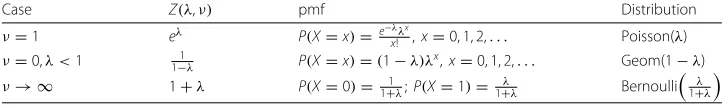
Table 1Well-known distributions associated with the Conway-Maxwell-Poisson (CMP) distribution for special cases ofλandν
Case Z(λ,ν) pmf Distribution
ν=1 eλ P(X=x)= e−xλ!λx,x=0, 1, 2,. . . Poisson(λ) ν=0,λ <1 1−1λ P(X=x)=(1−λ)λx,x=0, 1, 2,. . . Geom(1−λ)
theory (Sellers 2012; Saghir and Lin 2014a; 2014b), stochastic processes (Zhu et al. 2017), and multivariate data analysis (Sellers et al. 2016). The model has further been applied for various data problems including fitting word lengths (Wimmer et al. 1994), modeling online sales (Boatwright et al. 2003; Borle et al. 2006) and customer behavior (Borle et al. 2007), analyzing traffic accident data (Lord et al. 2008), and for use as a disclosure limita-tion procedure to protect individual privacy (Kadane et al. 2006). See Sellers et al. (2011) for additional overview and discussion.
3 The sum of Conway-Maxwell-Poissons (sCMP) class of distributions and its statistical properties
The sum of m independent and identically distributed (iid) CMP variables leads to what will be termed asum of Conway-Maxwell-Poissons (sCMP)(λ,ν,m) class of dis-tributions. Theorem 1 defines the three-parameter structure for some generalized rate parameter (λ), dispersion parameter (ν), and number of underlying CMP random variables (m).
Theorem 1. The sCMP(λ,ν,m)distribution has the following pmf for a random variable
Y =
m
i=1
Xi, where Xi iid
∼CMP(λ,ν):
P(Y =y|λ,ν,m)= λ
y
(y!)νZm(λ,ν) y
x1,...,xm=0 x1+···+xm=y
y x1· · ·xm
ν
, y=0, 1, 2,. . ., (7)
wherex y
1···xm
= y!
x1!···xm!is the multinomial coefficient.
ProofWe prove this result by induction. Form = 2, letXi ∼CMP(λ,ν),i= 1, 2 and
Y = X1+X2. Then, the result holds by the transformation technique (see Chapter 2 of Casella and Berger (2002)). Similarly, given that the result is true form=k−1, we can likewise apply the transformation technique to show that
P(Y =y) =
xk
λy−xk
[(y−xk)! ]νZk−1(λ,ν)·
y−xk
x1,...,xk−1=0 x1+···+xk−1=y−xk
y−xk
x1· · ·xk−1
ν λxk
(xk!)νZ(λ,ν)
= λy
Zk(λ,ν) y
x1,...,xk=0 x1+···+xk=y
[(y−xk)! ]ν
[(y−xk)! ]ν(xk!)ν(x1!· · ·xk−1!)ν ·
y!
y!
ν
= λy
(y!)νZk(λ,ν) y
x1,...,xk=0 x1+···+xk=y
y x1· · ·xk
ν .
The sCMP(λ,ν,m) class encompasses the Poisson distribution with rate parameter
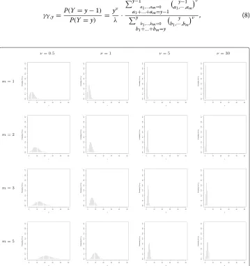
Figures 1 and 2 display the sCMP class for different values of m = 1, 2, 3, 5 and
ν = 0.5, 1, 5, 30 forλ= 2 (Fig. 1) andλ= 0.25 (Fig. 2), respectively. Both figures illus-trate the right skewness of the distribution, and show that the range of the data decreases asνincreases. Figure 1 more clearly demonstrates howmandνinfluence the centrality and shape of the distribution whenλ=2. As previously discussed, the special case where
ν=1 simplifies the sCMP(λ,ν,m) model to the Poisson(mλ) distribution. This illustrative example thus displays Poisson models with respective means equal-ing 4, 6, and 10. The increased variation in the respective figures is consis-tent with the increased shift in the distribution mean; recall that the Poisson mean and variance equal each other. Relative to the Poisson model, we see that (for a given m) increasing ν associates with decreasing variation. Figure 1 dis-plays longer tail distributions relative to the Poisson distribution for ν <1 and shorter tails relative to the Poisson model when ν >1. Meanwhile (for a given ν), increasingm clearly associates with increased shifts in the measures of distributional centrality (i.e. mean, median, and mode).
The ratio between probabilities of two consecutive values is
γY,y=
P(Y =y−1)
P(Y=y) =
yν
λ ·
y−1
a1,...,am=0
a1+...+am=y−1 y−1
a1,···,am ν
y
b1,...,bm=0
b1+...+bm=y
y
b1,···,bm
ν , (8)
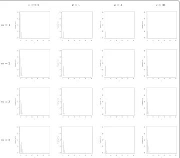
Fig. 2sCMP Probability Mass Functions. Collection of probability mass function figures for sCMP(λ=0.25,ν,m) distributions with varying values forν=0.5, 1, 5, 30 andm=1, 2, 3, 5
where the ratio of sums drops out in the special case wherem = 1 (i.e. one CMP(λ,ν) random variable); clearly, this produces the special case shown in Eq. (6). For the spe-cial case whereν = 1,γY,y = mλy , which is the linear form property of the Poisson random variable with parametermλ(i.e. the distribution of the sum ofmPoisson ran-dom variables). Meanwhile, for ν = 0,γY,y = λ(m+yy−1), namely the form associated with a negative binomial distribution (i.e. the sum of mgeometric random variables). Equation (8) implies that the sCMP model has a mode at 0 whenγY,y > 1, i.e. λ <
yν · y−1
a1,...,am=0 a1+...+am=y−1
( y−1 a1,···,am)
ν
y b1,...,bm=0 b1+...+bm=y
( y b1,···,bm)
ν . In particular, γY,1 = P(YP(Y==10)) = mλ1 , thus sCMP(λ,ν,m)
models whereλ < m1 have a mode at 0. Figure 2 displays the sCMP(λ = 0.25,ν,m) distributions for ν = 0.5, 1, 5, 30 and m = 1, 2, 3, 5. Given that λ = 0.25 = 14, we expect sCMP distributions where m < 4 to have the mode at 0. This is illus-trated accordingly in Fig. 2; sCMP(λ = 0.25,ν,m) distributions form = 2, 3 and any
ν ≥ 0 have the mode at 0, while the sCMP(λ = 0.25,ν,m = 5) distribution has the mode at 1 for allν≥0.
MY(t) =
Z(λet,ν)
Z(λ,ν)
m
, (9)
Y(t) =
Z(λt,ν)
Z(λ,ν)
m , and
φY(t) =
Z(λeit,ν)
Z(λ,ν)
m .
The moment generating function technique can be used to show that, given the same parameters λ and ν, the sum of independent sCMP distributions is invariant under addition (i.e. the sum of sCMP random variables has a sCMP distribution). For two independent random variables,Y1∼sCMP(λ,ν,m1)andY2∼sCMP(λ,ν,m2),
MY1+Y2(t) = MY1(t)·MY2(t)
= Zm1(λet,ν)
Zm1(λ,ν) ·
Zm2(λet,ν) Zm2(λ,ν)
= Zm1+m2(λet,ν)
Zm1+m2(λ,ν) ,
which is the mgf of a sCMP(λ,ν,m1 + m2) distribution, therefore Y1 + Y2 has a sCMP(λ,ν,m1 + m2) distribution. This result is logically sound because Y1 and Y2 respectively represent the sum ofm1 and m2 iid CMP (λ,ν) random variables; thus,
Y1+Y2defines the sum ofm1+m2iid CMP random variables, which precisely has a sCMP(λ,ν,m1+m2) distribution. This distinction is key between the CMP distribution and the larger sCMP class – the CMP distribution does not have the invariance property under addition.
3.1 Moments of the distribution
One can differentiate Eq. (9) to obtain the moments of the sCMP model, with the help of the following relation.
Theorem 2. For a normalizing function of the form, Z(λet,ν), where Z(·,·)is as defined following Eq. (2), the kth (k=1, 2, 3,. . .) derivative is
∂kZλet,ν
∂tk = ∞
j=0
jk
λetj
(j!)ν . (10)
ProofThis proof is straightforward, given the differentiation formula for exponential
functions.
This result proves helpful in showing that the sCMP(λ,ν,m) has mean E(Y) = mE(X)and varianceV(Y) = mV(X), whereE(X)andV(X) (provided in Eqs. (4)-(5), respectively) are the mean and variance of a CMP(λ,ν) random variableX.
3.2 Introducing the generalized Conway-Maxwell-Binomial (gCMB) distribution
Conditioning a CMP random variable on a sum of two independent CMP random variables produces a random variable whose distribution is Conway-Maxwell-Binomial (CMB) (Kadane 2016) (alternatively termed as “Conway-Maxwell-Poisson-Binomial” in Shmueli et al. (2005) and Borges et al. (2014)). The CMB random variableXhas the pmf,
P(X=x|r,p,ν)=
r
x
ν
px(1−p)r−x r
k=0
r
k
ν
forr ∈ Z+,p ∈ (0, 1), andν ∈ Rsuch thatν = 1 produces the usual binomial(r,p) distribution,ν >1 corresponds to data under-dispersion relative to a binomial distribu-tion whileν <1 corresponds to data over-dispersion relative to the binomial(r,p) model. Extreme distribution cases hold where, forν→ ∞, the pmf is concentrated at the point,
rpand, forν→ −∞, it is concentrated at 0 orr(Borges et al. 2014).
Analogously, conditioning a sCMP variable on the sum of two independent sCMP vari-ables produces a generalized form of the CMB distribution; we denote this as the gCMB distribution. LettingS=Y1+Y2whereY1∼sCMP(λ1,ν,m1)andY2∼sCMP(λ2,ν,m2) are independent, and givenS=s,
P(Y1=y1|S=s)=
⎧ ⎪ ⎪ ⎨ ⎪ ⎪ ⎩ s y1 ν λ 1
λ1+λ2
y1 λ
2
λ1+λ2
s−y1 ⎡ ⎢ ⎢ ⎣ y1
a1,...,am1=0
a1+...+am1=y1
y1
a1,. . .,am1 ν ⎤ ⎥ ⎥ ⎦ · ⎡ ⎢ ⎢ ⎢ ⎣
s−y1
b1,...,bm2=0
b1+...+bm2=s−y1
s−y1
b1,. . .,bm2 ν ⎤ ⎥ ⎥ ⎥ ⎦ ⎫ ⎪ ⎪ ⎪ ⎬ ⎪ ⎪ ⎪ ⎭ /G λ1
λ1+λ2
,ν,s,m1,m2
(12)
where
G(p,ν,s,m1,m2) = s
k=0
s k
ν
pk(1−p)s−k ⎡ ⎢ ⎢ ⎢ ⎣ k
a1,...,am1=0
a1+...+am1=k
k a1,. . .,am1
ν ⎤ ⎥ ⎥ ⎥ ⎦ · ⎡ ⎢ ⎢ ⎢ ⎣
s−k
b1,...,bm2=0
b1+...+bm2=s−k
s−k
b1,. . .,bm2 ν ⎤ ⎥ ⎥ ⎥ ⎦ (13)
is a normalizing constant and p = λ1
λ1+λ2. Thus, the conditional probability of a
sCMP(λ1,ν,m1) random variable given the value of a sum of sCMP random variables as described above is
P(Y1=y1|S=s) ∝
s y1
ν
py1(1−p)s−y1 ⎡ ⎢ ⎢ ⎣ y1
a1,...,am1=0
a1+...+am1=y1
y1
a1,. . .,am1 ν ⎤ ⎥ ⎥ ⎦ · ⎡ ⎢ ⎢ ⎢ ⎣
s−y1
b1,...,bm2=0
b1+...+bm2=s−y1
s−y1
b1,. . .,bm2 ν
⎤ ⎥ ⎥ ⎥
⎦. (14)
This generalized CMB distribution [denoted as gCMB(p,ν,s,m1,m2)] contains several special cases. Whenm1 = m2 = 1, the gCMB distribution reduces to the CMB(s,p,ν) distribution. Forν=1, the probability reduces to
P(Y1=y1|S=s) =
s
y1
(m1p)y1[m2(1−p)]s−y1 [m1p+m2(1−p)]s
=
s y1
m1p
m1p+m2(1−p)
y1 m
2(1−p)
m1p+m2(1−p)
s−y1
i.e. given data equi-dispersion, we have a binomial distribution withs trials andp∗ =
m1p
m1p+m2(1−p) =
m1λ1
m1λ1+m2λ2 success probability. In particular, for m1 = m2 = 1 and
ν=1, the gCMB distribution reduces to the Bin(s,p)= Bin
s, λ1
λ1+λ2 distribution. For
the special case whereλ1=λ2=λ, Eq. (12) reduces to the following fory1=0,. . .,s:
P(Y1=y1|S=s)=
s
y1 ν
y1
a1,...,am1=0
a1+...+am1=y1 y1
a1,...,am1 ν
⎡ ⎣s−y1
b1,...,bm2=0
b1+...+bm2=s−y1 s−y1
b1,...,bm2 ν
⎤ ⎦
s
c1,...,cm1+m2=0
c1+...+cm1+m2=s
s
c1,...,cm1+m2
ν ,
i.e. a gCMB(1/2,ν,s,m1,m2) distribution. In particular, this implies that
s
c1,...,cm1+m2=0
c1+...+cm1+m2=s
s c1,. . .,cm1+m2
ν =
s
y1=0 s y1 ν ⎡ ⎢ ⎢ ⎣ y1
a1,...,am1=0
a1+...+am1=y1
y1
a1,. . .,am1 ν ⎤ ⎥ ⎥ ⎦ · ⎡ ⎢ ⎢ ⎢ ⎣
s−y1
b1,...,bm2=0
b1+...+bm2=s−y1
s−y1
b1,. . .,bm2 ν ⎤ ⎥ ⎥ ⎥ ⎦.
The probability generating function for the gCMB distribution is
φY1|S=s(t) = s
y1=0 s
y1 ν(
tp)y1(1−p)s−y1y1
a1,...,am1 y1
a1,...,am1
νs−y1
b1,...,bm2 s−y1
b1,...,bm2 ν
G(p,ν,s,m1,m2)
= H
tp
1−p,ν,s,m1,m2
H
p
1−p,ν,s,m1,m2 ,
where
H(θ,ν,s,m1,m2)= s
y1=0
s y1
ν
θy1 ⎡ ⎣ y1
a1,...,am1
y1
a1,. . .,am1 ν⎤
⎦ ⎡ ⎣ s−y1
b1,...,bm2
s−y1
b1,. . .,bm2 ν⎤
⎦.
(15)
4 Parameter estimation and statistical computing
Becausemis a natural number, we consider a series of sCMP estimations for a givenm, from which we can determine an optimal sCMP(λ,ν,m) model. Givenm, estimates for
λandνare obtained via maximum likelihood estimation (MLE), where we consider the log-likelihood,
logL(λ,ν|m)=
N
i=1
logP(Yi=yi|λ,ν,m)
I(λ,ν)= −N·E
∂2lnP(Y=y)
∂λ2
∂2lnP(Y=y)
∂λ∂ν ∂2lnP(Y=y)
∂λ∂ν ∂
2lnP(Y=y)
∂ν2
,
where P(Y = y) is defined in Eq. (7). The information matrix is computed (via the hessianfunction in thenumDerivpackage (Gilbert and Varadhan 2016) inR(R Core Team 2017)) and inverted, and the square root of the resulting diagonal elements contain the standard errors of the parameter estimates.
Optimal sCMP(λ,ν,m) models are determined by comparing potential conditional sCMP models wherem is assumed known and identifying the conditional model with the largest log-likelihood value. Section 5 illustrates this procedure via simulated and real data examples.
Statistical computing for the Poisson and negative binomial distributions are conducted in R(R Core Team 2017) via the function, fitdistr, contained in the MASS pack-age (Venables and Ripley 2002). This packpack-age uses an alternative parametrization for the negative binomial model, namely θ = n and μ = n(1p−p), hence we can back-solve for p = μ+θθ. Estimates for θ and μ are reported in the discussions provided in Section 5.
5 Examples
5.1 Simulation study
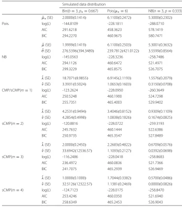
The sCMP distribution is a generalizable distribution that encompasses five classical distributions: the Bernoulli, binomial, Poisson, geometric, and negative binomial distri-butions; more broadly, for a general m, the sCMP distribution captures the binomial, Poisson, and negative binomial distributions. To demonstrate this general flexibility, data samples of size 100 were generated from a binomial(b=3,p∗=0.667), Poisson(μ∗=6), and negative binomial(n = 3, p = 0.333) distribution, respectively. To assess model performance, we compare model estimation via the sCMP distribution (assumingm =
1, 2, 3, 4) with estimations assuming a Poisson and negative binomial distribution, respec-tively; the CMP distribution is the sCMP(m = 1) case. Table 2 provides the parameter estimates and standard errors associated with the various models considered for model comparisons via the log-likelihood (log(L)), Akaike and Bayes Information Criterions (AIC and BIC), respectively.
For model comparison via AIC, Burnham and Anderson (2002) suggest considering
i=AICi−AICmin, whereAICminis the minimum of the model AIC values being com-pared, thus infering that the best model has = 0 and the other models have > 0. Model comparisons are thus determined via these difference measures in that “models having i ≤ 2 have substantial support (evidence), those in which 4 ≤ i ≤ 7 have considerably less support, and models having i > 10 have essentially no support" in comparison with the best model; see p. 70-71 of Burnham and Anderson (2002). We will apply this approach for model comparison accordingly, and can analogously apply this method using BIC.
Table 2Simulated data example
Simulated data distribution
Bin(b=3,p∗=0.667) Pois(μ∗=6) NB(n=3,p=0.333) ˆ
μ∗(SE) 2.0000(0.1414) 6.1100(0.2472) 5.3000(0.2302) Pois. log(L) -144.8109 -228.1811 -288.0710
AIC 291.6218 458.3623 578.1419 BIC 294.2270 460.9675 580.7471
ˆ
μ(SE) 1.9999(0.1419) 6.1100(0.2503) 5.3001(0.3632) ˆ
θ(SE) 276.5396(394.3489) 239.7812(421.0122) 3.5599(0.8564) NB log(L) -145.0563 -228.3236 -258.7486
AIC 294.1126 460.6472 521.4971 BIC 299.3229 465.8575 526.7075 ˆ
λ(SE) 18.7071(8.9855) 6.9145(2.1193) 1.5576(0.2079) ˆ
ν(SE) 3.3931(0.5024) 1.0653(0.1603) 0.3150(0.0708) CMP/sCMP(m=1) log(L) -123.2624 -228.0950 -260.3649
AIC 250.5248 460.1900 524.7298 BIC 255.7351 465.4003 529.9402 ˆ
λ(SE) 4.2531(0.9494) 3.4046(0.8152) 0.9309(0.1109) ˆ
ν(SE) 4.2854(0.4998) 1.0838(0.1826) 0.1674(0.0825) sCMP(m=2) log(L) -120.8816 -228.0722 -259.3193
AIC 245.7632 460.1444 522.6386 BIC 250.9735 465.3547 527.8489 ˆ
λ(SE) 2.0000(0.2450) 2.2683(0.4822) 0.6709(0.0576) ˆ
ν(SE) 33.6942(12536.57) 1.1093(0.2127) 0.0392(0.0698) sCMP(m=3) log(L) -116.2486 -228.0418 -258.8683
AIC 236.4972 460.0836 521.7366 BIC 241.7075 465.2939 526.9469 ˆ
λ(SE) 1.0000(0.1000) 1.7044(0.3382) 0.5700(0.0486) ˆ
ν(SE) 32.5126(12322.57) 1.1381(0.2469) 0.0000(0.0826) sCMP(m=4) log(L) -124.7123 -228.0175 -258.8470
AIC 253.4246 460.0350 521.6940 BIC 258.6349 465.2453 526.9043
True model parameters versus estimated parameters (and associated standard errors provided in parentheses) for various assumed distributions. For model comparisons, the log-likelihood, Akaike and Bayes Information Criterions (AIC and BIC, respectively) are provided
pattern does not continue form = 4, we see that the log-likelihood value is maximized (and the AIC and BIC values minimized) with the sCMP(m = 3) case. We see that the sCMP(λˆ =2.0000,νˆ = 33.6942,m=3) distribution is the best model, when compared with the other considered distributions. In fact, all other models produce a difference that associates with considerably less support to essentially no support.
The binomial case can be viewed as the summation of three Bernoulli trials, thus we expect the corresponding sCMP estimates to beλˆ ≈ 2 andνˆ ≥30; recall that the spe-cial CMP case that corresponds with a Bernoulli distribution occurs whenν→ ∞with probability 1+λλ, where empirical evidence shows that dispersion parameter estimation is sufficiently achieved whenνˆ ≈30 or more (see Sellers et al. (2016) and Sellers and Raim (2016) for examples). In fact, for the simulated Binomial dataset, we obtainλˆ =2.0000, ˆ
success probability,pˆ∗ = 1+2.00002.0000 = 0.6667. The sCMP(m = 3) distribution best mod-els the binomial data, producing the largest log-likelihood (log(L)= −116.2486), and the smallest AIC and BIC (236.4972 and 241.7075, respectively). In comparison, the Poisson and negative binomial models produce comparable log-likelihoods (both that are con-siderably less than those from the sCMP class) because they are unable to effectively model the under-dispersion present in this dataset. The large negative binomial param-eter (θˆ= 276.5396) shows that the model is converging to a Poisson model (i.e. towards data equi-dispersion) to estimate this data. While the CMP model is able to recognize the dataset as being under-dispersed (νˆ=3.3931>1), the form of the distribution still limits the amount of model flexibility it can address.
For the Poisson example, we see that all of the considered models perform comparably well. While the best model is naturally Poisson, this is true moreso because the distri-bution only requires estimating one parameter. All of the models considered produced log-likelihoods equalling approximately−228, thus the associated difference measures imply that the other models (in particular, the sCMP class of distributions) show sub-stantial support for model consideration. The negative binomial estimates (θˆ=239.7812 and μˆ = 6.1100) demonstrate the convergence of the negative binomial distribution to the Poisson model as θ → ∞ in order to address the limiting case of analyzing equi-dispersed data.
Because the simulation reflects a Poisson(6) dataset, we expect to obtain sCMP param-eter estimatesλˆ ≈6/mandνˆ ≈1 for allm=1, 2, 3, 4. The obtained estimates forλandν are consistently larger than their projected values whereνˆincreases slightly withm. The corresponding parameter standard errors, however, suggest that none of these estimates is statistically significantly different from their hypothesized values.
For the negative binomial example, we see that the sCMP class of distributions again performs well in estimating the form of the simulated dataset. The true parameter val-ues associated with the negative binomial model imply thatμ= n(1p−p) = 6 andθ =3. The negative binomial distribution(θˆ = 3.5599,μˆ = 5.3001) is the best model among the distributions considered (AIC = 521.4971), however, the sCMP class of distribu-tions performs more optimally asmincreases (among those values formconsidered). Larger values formwere not considered here because the sCMP models form = 3, 4 produce approximately equal log-likelihood values, thus likewise producing compara-ble AIC and BIC values; this makes sense because the negative binomial estimate is 3 < θˆ = 3.5599 < 4. Meanwhile, even for the sCMP models wherem = 1, 2, the dif-ference in AIC when compared with the best model still implies that these models show considerable support.
With the sCMP class of distributions, we see thatνˆ decreases asmincreases. Inter-estingly here, because we know the data are simulated from a negative binomial(n =
3,p=0.333) distribution, we expect the sCMP(m=3) distribution to produce estimates ˆ
λ = 0.667 andν ≈ 0. In fact, the observed estimates (λˆ = 0.6709 andνˆ = 0.0392) are within one standard error of the projected estimates. The CMP (i.e. the sCMP(m = 1)) model does reasonably well, as evidenced by the resulting log-likelihood and AIC val-ues (−260.3649 and 524.7298, respectively); the CMP estimated dispersion parameter, ˆ
5.2 Under-dispersed real data example: word count
Bailey (1990) studies the frequency of articles in 10-word samples from Macaulay’s “Essay on Milton”, counting the number of occurrences of articles ‘the’, ‘a’, and ‘an’ as a means to infer the author’s style. The provided dataset contains 100 observations where the number of occurrences of these articles in the 10-word samples range from 0 to 3; see Fig. 3.
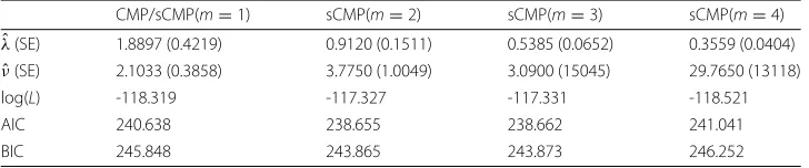
We consider the Poisson, negative binomial, and sCMP(m) models wherem=1, 2, 3, 4 to describe the data distribution; Bailey (1990) previously considered a binomial model to describe the data. Table 3 provides the sCMP parameter estimates and standard errors (in parentheses), along with the log-likelihood, AIC, and BIC values for model compari-son. The sCMP(m=2) model is the optimal choice, producing a log-likelihood equaling −117.327, and AIC and BIC equaling 238.6546 and 243.8649, respectively. Because this dataset is under-dispersed (with a sample mean and sample variance equaling 1.05 and 0.654, respectively), all models considered from the sCMP family outperform the Pois-son and negative binomial models. The PoisPois-son model produces an estimated sample mean and standard error, 1.0500 (0.1025), with log-likelihood−123.2741. The negative
Table 3Word count model comparisons
CMP/sCMP(m=1) sCMP(m=2) sCMP(m=3) sCMP(m=4) ˆ
λ(SE) 1.8897 (0.4219) 0.9120 (0.1511) 0.5385 (0.0652) 0.3559 (0.0404) ˆ
ν(SE) 2.1033 (0.3858) 3.7750 (1.0049) 3.0900 (15045) 29.7650 (13118) log(L) -118.319 -117.327 -117.331 -118.521
AIC 240.638 238.655 238.662 241.041
BIC 245.848 243.865 243.873 246.252
Model comparison for the word count data from Bailey (1990), where sCMP withm=1, 2, 3, 4 distributions are considered. For model comparisons, the log-likelihood, Akaike and Bayes Information Criterions (AIC and BIC, respectively) are provided. All sCMP family distributions outperform the Poisson model which produces an estimated sample mean,μ∗=1.0500 (0.1025), with log-likelihood−123.2741. The negative binomial model likewise converges to a Poisson model with estimates,θˆ=269.9607 (702.1046),μˆ=1.0500 (0.1027), log(L)= −123.3487)
binomial model meanwhile produces estimates (θˆ = 269.9607 (702.1046),μˆ = 1.0500 (0.1027), log(L) = −123.3487)comparable to the Poisson. Because the data are under-dispersed, the negative binomial model can only perform as well as the Poisson model. As demonstrated, the estimated size parameter is large and the estimated mean equals that from the Poisson model.
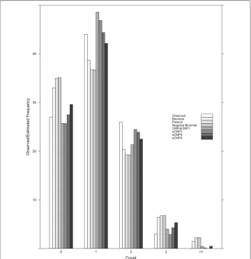
Figure 3 provides the empirical and estimated distributions for this data based on the various considered models, including the estimated binomial frequencies provided in Bailey (1990). This figure confirms the results provided in Table 3, namely that the sCMP(m = 2) best represents the shape of the observed distribution for the num-ber of occurrences of an article in 10-word samples from Macaulay’s ‘Essay on Milton’. In particular, we see the small estimated sCMP(m = 2) frequency associated with more than 3 articles; recall that the observed number of articles is zero. Meanwhile, the number of occurrences as determined via the Poisson and negative binomial are visi-bly over- or under-estimated, including a sizable estimated frequency associated with more than 3 articles. The estimated frequencies determined by the binomial distri-bution, while better than those from the Poisson and negative binomial models, still deviate considerably in comparison to the sCMP class. Finally, while Table 3 shows that the sCMP(m = 3) distribution performs comparably well, we nonetheless deter-mine the sCMP(λˆ = 0.9120,νˆ = 3.7750,m = 2) model to be the best choice to estimate the observed distribution, based on the resulting estimated frequencies shown in Fig. 3.
5.3 Over-dispersed real data example: fetal lamb movement
Guttorp (1995) provides data on the number of movements by a fetal lamb observed by ultrasound and counted in successive 5-second intervals. The dataset contains 225 observations ranging in value from 0 to 7, and are over-dispersed with dispersion index
Table 4Fetal lamb summary statistic information
(a) (b)
5-second 15-second
Summary statistic Data value Data value
No. of obs. 225 75
Minimum 0.000 0.000
1st Quartile 0.000 0.000
Median 0.000 1.000
Mean 0.382 1.147
3rd Quartile 1.000 2.000
Maximum 7.000 12.000
Variance 0.693 3.694
Std. Deviation 0.832 1.922
Summary statistics associated with fetal lamb data set: (a) based on original data, where fetal lamb are observed by ultrasound and counted in successive 5-second intervals, and (b) based on reconstructed (from original) data, where fetal lamb are observed by ultrasound and counted in successive 15-second intervals. Full original data are contained in Guttorp (1995)
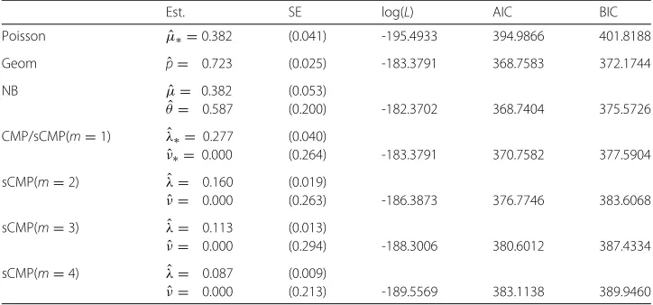
The sCMP class consistently recognizes this real count distribution to be extremely over-dispersed (νˆ = 0.000 andλ <1), implying that the sCMP class interprets the data as being represented as sums of sizemfrom geometrically distributed data with some success probability, 1− ˆλ. In fact, the estimates forλdecrease asmincreases yet the cor-responding log-likelihood value decreases, thus providing a sense of the contour of the larger log-likelihood space that is determined byλ,ν, andm. Becausemis a natural num-ber, we find that the optimal sCMP(m) class for modeling the 5-second fetal lamb dataset occurs form = 1, i.e. the CMP distribution withλˆ = 0.277 andνˆ = 0.000. Continuing with this logic, however, we recognize then that one should thus consider the special case of a geometric (i.e. the CMP distribution whereν = 0) distribution with approximate success probability,pˆ =1−0.277=0.723). Indeed, estimating the observed count distri-bution via a geometric model produces the estimated success probability,pˆ=0.723 (with standard error, 0.025). While this estimation procedure determines a geometric model to be the best model within the sCMP class, the negative binomial distribution is another viable model, as determined by Burnham and Anderson (2002); see Table 5.
Table 55-second fetal lamb data model comparisons
Est. SE log(L) AIC BIC
Poisson μˆ∗=0.382 (0.041) -195.4933 394.9866 401.8188 Geom pˆ= 0.723 (0.025) -183.3791 368.7583 372.1744 NB μˆ= 0.382 (0.053)
ˆ
θ= 0.587 (0.200) -182.3702 368.7404 375.5726 CMP/sCMP(m=1) λˆ∗= 0.277 (0.040)
ˆ
ν∗= 0.000 (0.264) -183.3791 370.7582 377.5904 sCMP(m=2) λˆ= 0.160 (0.019)
ˆ
ν= 0.000 (0.263) -186.3873 376.7746 383.6068 sCMP(m=3) λˆ= 0.113 (0.013)
ˆ
ν= 0.000 (0.294) -188.3006 380.6012 387.4334 sCMP(m=4) λˆ= 0.087 (0.009)
ˆ
ν= 0.000 (0.213) -189.5569 383.1138 389.9460
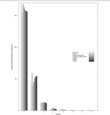
Figure 4 provides a comparison of the empirical versus estimated count distributions associated with the different models. While the negative binomial best fits the observed count distribution, we see that the geometric (pˆ = 0.723) (i.e. the sCMP(m = 1)/CMP model withλˆ = 0.277 andνˆ =0.000) model likewise performs reasonably. More gener-ally, asmincreases, the sCMP class appears to underestimate the number of zeroes and overestimate the number of ones. The estimated frequencies for counts greater than or equal to two, however, appear comparable for all distributions.
To further illustrate the utility of the sCMP family, we consider a condensed represen-tation of the Guttorp (1995) data by summing successive triples of data, thus representing fetal lamb data observed by ultrasound and counted in successive 15-second intervals. Table 4(b) provides the resulting summary information – 75 observations now range in value from 0 to 12, where the dispersion index is now 3.694/1.147 = 3.221, maintaining apparent data over-dispersion. Again, assuming no knowledge regarding the type of the data dispersion, we consider the Poisson, negative binomial, and sCMP distributions at
m=1, 2, 3, 4 and estimate the corresponding model parameters via maximum likelihood
estimation. Table 6 provides the resulting estimation output (including the corresponding log-likelihood, AIC, and BIC) associated with the various distributions considered to model the 15-second movement data summarized in Table 4(b).
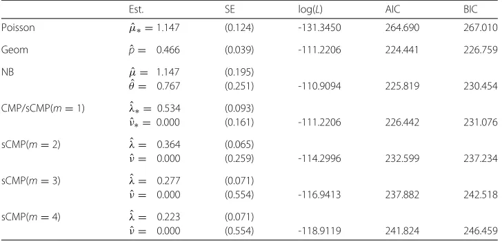
Table 6 again displays an interesting trend with respect to the sCMP class estimators. Again, the estimations for λ decrease as mincreases, while the dispersion parameter consistently estimates to be νˆ = 0 (indicating consideration of an appropriate nega-tive binomial model structure). Further, asmincreases, the corresponding log-likelihood associated with each of the models decreases. Hence, the optimal sCMP model is again the CMP model (i.e. sCMP whenm = 1). Meanwhile, the CMP model with estimated dispersion parameter,νˆ =0, again suggests to consider a geometric model with success probability 1− ˆλ = 0.466. In fact, the estimated success probability for the geometric model ispˆ =0.466(0.039). The negative binomial model slightly outperforms the CMP model, although both models perform comparably well, based on their respective AIC values (Burnham and Anderson 2002). The slight outperformance in the negative bino-mial model relative to the CMP/geometric model (based on log-likelihood comparisons) stems from the negative binomial estimation procedure’s allowance for realθ, thus obtain-ing a more precise estimation of the data over-dispersion. However, because we recognize that this special case of the sCMP class wherem = 1 andν = 0 corresponds to a geo-metric model, the geogeo-metric model is deemed better than the negative binomial model, given the reduction in the number of estimated parameters and thus the reduced AIC and BIC (224.441 and 226.759 for the geometric model, versus 225.819 and 230.454 for the negative binomial model); see Table 6.
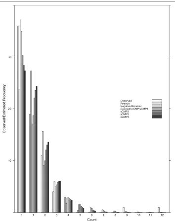
Figure 5 provides a comparison of the empirical versus estimated count distributions for the different models associated with the 15-second fetal lamb data. Here, we can see that the geometric(pˆ = 0.466) distribution (i.e. the sCMP(m = 1)/CMP model where ˆ
λ=0.534,νˆ =0.000) best estimates the observed count distribution, given that the geo-metric model requires only one parameter. Meanwhile, the negative binomial distribution performs comparably well to the geometric/CMP(νˆ = 0). This makes sense, given the relationship between the geometric and negative binomial distributions. The estimated geometric and negative binomial distributions are so close because the negative binomial
Table 615-s fetal lamb data model comparisons
Est. SE log(L) AIC BIC
Poisson μˆ∗=1.147 (0.124) -131.3450 264.690 267.010 Geom pˆ= 0.466 (0.039) -111.2206 224.441 226.759
NB μˆ= 1.147 (0.195)
ˆ
θ= 0.767 (0.251) -110.9094 225.819 230.454 CMP/sCMP(m=1) λˆ∗= 0.534 (0.093)
ˆ
ν∗= 0.000 (0.161) -111.2206 226.442 231.076 sCMP(m=2) λˆ= 0.364 (0.065)
ˆ
ν= 0.000 (0.259) -114.2996 232.599 237.234 sCMP(m=3) λˆ= 0.277 (0.071)
ˆ
ν= 0.000 (0.554) -116.9413 237.882 242.518 sCMP(m=4) λˆ= 0.223 (0.071)
ˆ
ν= 0.000 (0.554) -118.9119 241.824 246.459
Fig. 515-second fetal lamb distribution comparison. Empirical versus estimated count distributions for 15-second fetal lamb data example as described in Section 5.3. Estimated count distributions determined from corresponding model parameter estimates provided in Table 6
size estimate,θˆ = 0.767, is close to one, while the corresponding probability estimate, ˆ
p=0.401, is close to that from the geometric model (pˆ =0.466).
Notice that sCMP(m = 3) parameter estimates associated with the 15-second fetal lamb data equal the sCMP(m=1)/CMP parameter estimates for the 5-second fetal lamb example. This result is logically sound, given the means by which the sCMP distribution is derived; conducting estimations over an interval that is three times its original period is akin to “summing" the three CMP random variables to consider the sCMP model.
distribution is generally expected to be a good model to describe the distribution. The sCMP class of distributions contains the negative binomial (and geometric) distribution as a special case; accordingly, it is not necessarily expected for the sCMP distribution to outperform simpler distributions but rather to demonstrate that the sCMP distribution offers insights regarding model considerations. Indeed, applying the sCMP model to these over-dispersed examples motivated consideration of the geometric distribution, which turned out to be an optimal model. Accordingly, while one may not consider the geomet-ric distribution to be a viable model a priori, the sCMP showed why the geometgeomet-ric model is viable.
6 Discussion
The sum-of-Conway-Maxwell-Poissons (sCMP) class of distributions is a flexible con-struct for modeling count data that captures several well-known distributions as special cases: the Poisson, negative binomial, binomial, geometric, Bernoulli, and Conway-Maxwell-Poisson (CMP). Just as the CMP distribution bridges the gap between the Poisson, geometric, and Bernoulli distributions through the addition of a dispersion parameter, the sCMP distribution sums overm CMP random variables, producing an encompassing distributional form that has an even greater containment of numerous count distributions.
The provided examples illustrate the flexibility of the sCMP class for handling over-or under-dispersed data. These examples, however, consider only the marginal distribu-tion through uncondidistribu-tional means and variances (and hence uncondidistribu-tional dispersion), thus the true significance of the sCMP class is subdued. In actuality, it is not necessarily straightforward to determine if observed dispersion is true or “apparent". In a regres-sion setting, for example, disperregres-sion is measured via conditional means and variances, and exploratory data analysis may not detect the true complexity of the data (Sellers and Shmueli 2013). Under such circumstances, the sCMP class can aid with detecting dispersion when a more sophisticated approach is required.
As noted in the over-dispersed data example, we are limited in our ability to esti-matembecause it is a natural number. We opt for this formulation as it holds true to the form that generalizes the construction of the three special case models (negative binomial, Poisson, and binomial) as sums of their respective special case distributions associated with the CMP distribution (namely, the geometric, Poisson, and Bernoulli models). For example, the negative binomial pmf is often described as the probability of observingyfailures before thenth success in a series of Bernoulli trials, or as a sum of ngeometric random variables. Yet, the negative binomial distribution can alterna-tively be derived via a Poisson-gamma mixture, in which case the parameternis a real number. As Hilbe (2008) notes, “there is no compelling mathematical reason to limit this parameter to integers." (page 82). Future work considers broadening the sCMP for-mulation to likewise allow for real-valuedmand any associated implications from such a definition.
While we estimate the standard errors of the parameter estimates via the approximate information matrix as described in Section 4, the sampling distributions associated with
replacement from the data using thebootpackage (Canty and Ripley 2015) inR(R Core Team 2017).
Acknowledgements
Support for Kimberly Sellers was provided in part by the American Statistical Association (ASA)/National Science Foundation (NSF)/Census Research Program, U. S. Census Bureau Contract #YA1323-14-SE-0122. Support for Andrew W. Swift was provided by a grant from the Simons Foundation (#359536). Support for Kimberly S. Weems was provided in part by the NSF grant #1700235. The authors thank the reviewers and Drs. Darcy S. Morris (U.S. Census Bureau) and Derek Young (University of Kentucky) for helpful comments regarding the manuscript.
Authors’ contributions
KFS conceived the study. KFS, AS, and KSW contributed to statistical methods and computational development, and analyses. All authors read and approved the final manuscript.
Competing interests
The authors declare no competing interests.
Publisher’s Note
Springer Nature remains neutral with regard to jurisdictional claims in published maps and institutional affiliations.
Author details
1Department of Mathematics and Statistics, Georgetown University, 306 St. Mary’s Hall, Washington, DC, 20057, USA. 2Department of Mathematics, University of Nebraska - Omaha, 6001 Dodge Street, Omaha 68182, NE, USA.3Department
of Mathematics and Physics, North Carolina Central University, 2211 Mary M. Townes Science Building, 1801 Fayetteville Street, Durham 27707, NC, USA.
Received: 23 December 2016 Accepted: 11 September 2017
References
Bailey, BJR: A model for function word counts. J. R. Stat. Soc. Ser. C.39(1), 107–114 (1990)
Boatwright, P, Borle, S, Kadane, JB: A model of the joint distribution of purchase quantity and timing. J. Am. Stat. Assoc.
98, 564–572 (2003)
Borges, P, Rodrigues, J, Balakrishnan, N, Bazán, J: A COM-Poisson type generalization of the binomial distribution and its properties and applications. Stat. Probab. Lett.87, 158–166 (2014)
Borle, S, Boatwright, P, Kadane, JB: The timing of bid placement and extent of multiple bidding: An empirical investigation using ebay online auctions. Stat. Sci.21(2), 194–205 (2006)
Borle, S, Dholakia, U, Singh, S, Westbrook, R: The impact of survey participation on subsequent behavior: An empirical investigation. Mark. Sci.26(5), 711–726 (2007)
Burnham, KP, Anderson, DR: Model Selection and Multimodel Inference. Springer, New York (2002)
Canty, A, Ripley, B:Boot: Bootstrap Functions. 1.3-15 edn (2015). http://cran.r-project.org/web/packages/boot/index.html Casella, G, Berger, RL: Statistical Inference, Second Edition. Duxbury, Pacific Grove (2002)
Conway, RW, Maxwell, WL: A queuing model with state dependent service rates. J. Ind. Eng.12, 132–136 (1962) Gilbert, P, Varadhan, R: NumDeriv: Accurate Numerical Derivatives. 2016.8-1 edn (2016). https://cran.r-project.org/web/
packages/numDeriv/index.html
Guttorp, P: Stochastic Modeling of Scientific Data. Chapman & Hall/CRC, Boca Raton (1995) Hilbe, JM: Negative Binomial Regression. Cambridge University Press, United Kingdom (2008)
Kadane, JB, Krishnan, R, Shmueli, G: A data disclosure policy for count data based on the COM-Poisson distribution. Manag. Sci.52(10), 1610–1617 (2006)
Kadane, JB: Sums of possibly associated Bernoulli variables: The Conway-Maxwell-Binomial distribution. Bayesian Anal.
11(2), 403–420 (2016)
Lord, D, Guikema, SD, Geedipally, SR: Application of the Conway-Maxwell-Poisson generalized linear model for analyzing motor vehicle crashes. Accid. Anal. Prev.40(3), 1123–1134 (2008)
Minka, TP, Shmueli, G, Kadane, JB, Borle, S, Boatwright, P: Computing with the COM-Poisson distribution. Technical Report 776, Dept. of Statistics, Carnegie Mellon University (2003). http://www.stat.cmu.edu/tr/tr776/tr776.pdf
R Core Team: R: A language and environment for statistical computing. R Foundation for Statistical Computing, Vienna (2017). https://www.R-project.org/
Saghir, A, Lin, Z: Cumulative sum charts for monitoring the COM-Poisson processes. Comput. Ind. Eng.68, 65–77 (2014) Saghir, A, Lin, Z: A flexible and generalized exponentially weighted moving average control chart for count data. Qual.
Reliab. Eng. Int.30(8), 1427–1443 (2014)
Sellers, KF, Shmueli, G, Borle, S: The COM-Poisson model for count data: a survey of methods and applications. Appl. Stoch. Model. Bus. Ind.28, 104–116 (2011)
Sellers, K: A distribution describing differences in count data containing common dispersion levels. Adv. Appl. Stat. Sci.
7(3), 35–46 (2012)
Sellers, KF, Shmueli, G: A regression model for count data with observation-level dispersion. In: Booth, JG (ed.) Proceedings of the 24th International Workshop on Statistical Modelling, pp. 337–344. Cornell University Press, Ithaca, (2009) Sellers, KF, Shmueli, G: Data dispersion: Now you see it... now you don’t. Commun. Stat. Theory Methods.42, 1–14 (2013) Sellers, KF: A generalized statistical control chart for over- or under-dispersed data. Qual. Reliab. Eng. Int.28(1), 59–65
(2012)
Sellers, KF, Shmueli, G: A flexible regression model for count data. Ann. Appl. Stat.4(2), 943–961 (2010)
Sellers, KF, Morris, DS, Balakrishnan, N: Bivariate Conway-Maxwell-Poisson distribution: Formulation, properties, and inference. J. Multivar. Anal.150, 152–168 (2016)
Shmueli, G, Minka, TP, Kadane, JB, Borle, S, Boatwright, P: A useful distribution for fitting discrete data: revival of the Conway-Maxwell-Poisson distribution. Appl. Stat.54, 127–142 (2005)
Venables, WN, Ripley, BD: Modern Applied Statistics with S. 4th edn. Springer, New York (2002)
Wimmer, G, Köhler, R, Frotjahn, R, Altmann, G: Towards a theory of word length distribution. J. Quant. Linguist.1(1), 98–106 (1994)
Zhu, L, Sellers, KF, Morris, DS, Shmuéli, G: Bridging the gap: A generalized stochastic process for count data. Am. Stat.