R E S E A R C H
Open Access
Evaluation of noise robustness for local binary
pattern descriptors in texture classification
Gustaf Kylberg
1and Ida-Maria Sintorn
2*Abstract
Local binary pattern (LBP) operators have become commonly used texture descriptors in recent years. Several new LBP-based descriptors have been proposed, of which some aim at improving robustness to noise. To do this, the thresholding and encoding schemes used in the descriptors are modified. In this article, the robustness to noise for the eight following LBP-based descriptors are evaluated; improved LBP, median binary patterns (MBP), local ternary patterns (LTP), improved LTP (ILTP), local quinary patterns, robust LBP, and fuzzy LBP (FLBP). To put their performance into perspective they are compared to three well-known reference descriptors; the classic LBP, Gabor filter banks (GF), and standard descriptors derived from gray-level co-occurrence matrices. In addition, a roughly five times faster implementation of the FLBP descriptor is presented, and a new descriptor which we call shift LBP is introduced as an even faster approximation to the FLBP. The texture descriptors are compared and evaluated on six texture datasets; Brodatz, KTH-TIPS2b, Kylberg, Mondial Marmi, UIUC, and a Virus texture dataset. After optimizing all parameters for each dataset the descriptors are evaluated under increasing levels of additive Gaussian white noise. The
discriminating power of the texture descriptors is assessed using tenfolded cross-validation of a nearest neighbor classifier. The results show that several of the descriptors perform well at low levels of noise while they all suffer, to different degrees, from higher levels of introduced noise. In our tests, ILTP and FLBP show an overall good
performance on several datasets. The GF are often very noise robust compared to the LBP-family under moderate to high levels of noise but not necessarily the best descriptor under low levels of added noise. In our tests, MBP is neither a good texture descriptor nor stable to noise.
1 Introduction
The texture of objects in digital images is an important property utilized in many computer vision and image analysis applications such as face recognition, object clas-sification, and segmentation. Despite its frequent use and the many attempts to describe it in general terms, texture lacks a precise definition. This makes the development of new texture descriptors an ill-posed problem [1,2]. The recent textbook by Pietikäinen et al. [3] provide a good description of texture in stating that “A textured area in an image can be characterized by a non-uniform or varying spatial distribution of intensity or color”.
Local binary patterns (LBPs) emerged in the mid-1990s. At first, they were introduced as a local contrast descriptor
*Correspondence: [email protected]
2Centre for Image Analysis, Swedish University of Agricultural Sciences, Uppsala, Sweden
Full list of author information is available at the end of the article
[4] and a further development of the texture spectra intro-duced in [5]. Shortly thereafter, LBP was shown to be an interesting texture descriptor [6]. Many extensions to the classic LBP have since then been proposed. A comprehen-sive book about the LBP family of texture descriptors was recently published [3]. While some propositions focus on different sampling patterns to effectively capture the char-acteristics of certain textures, others propose descriptors focusing on improving the robustness to noise by using different encoding or thresholding schemes. The latter group is the focus of this article; considering LBP-based descriptors where the thresholding and encoding schemes are modified to create more noise robust descriptors.
Although several new LBP-based texture descriptors have been published, there is a limited number of compar-ative studies and evaluations. However, the recent study in [7], and the previous study by the same authors in [8], together cover six datasets from different applica-tions, mainly in the biomedical area. They report results
achieved using different sampling patterns and thresh-olding schemes as well as combinations of LBP-based descriptors with integrated ensembles of support vector machine (SVM) classifiers. The parameter values explored are limited and the focus is on optimizing combinations of LBP-based descriptors that work well for several types of texture datasets. Another recent survey is [9] where a large number of LBP-based descriptors are compared and put into a unifying framework called histograms of equiv-alent patterns (HEP). These descriptors are evaluated on 11 general texture datasets and the descriptors are then ranked based on pairwise comparisons of the classifica-tion results in the pursuit for the overall best descriptor in the HEP framework.
Unlike the previously mentioned surveys the aim of this article is to evaluate the noise robustness of a num-ber of LBP-based descriptors. The selected descriptors are all designed to be noise robust alternatives to the original LBP by altering the thresholding or encod-ing scheme. The descriptors are namely improved LBP (ILBP), median binary patterns (MBP), local ternary pat-terns (LTP), improved local ternary patpat-terns (ILTP), local quinary patterns (LQP), robust LBP (RLBP), shift LBP (SLBP), and fuzzy/soft LBP (FLBP). The SLBP descriptor is proposed in this article as a fast and simple approxi-mation to FLBP. The discriminating power of the texture descriptors are evaluated by applying them to six differ-ent texture datasets followed by a cross-validated classi-fication using a first nearest neighbor classifier (1-NN). Before the noise robustness is assessed all the descriptors parameters are thoroughly optimized, exploring a search space larger than a few combinations of parameter values, which is commonly the case reported in the literature.
When using LBP, it is quite common to exclude the specificity of the so-called non-uniform patterns and count their occurrences as simply non-uniform [10]. In brief, binary codes with more transitions between ‘0’ and ‘1’ than a specific value (typically two) are called non-uniform. In this way, the number of possible binary codes decreases but at the same time some important informa-tion may be lost, see for example [10,11]. This is why both uniform and non-uniform binary codes are considered in this article.
To put the performance of the LBP-based descriptors into perspective they are compared to the classical LBP, a set of Gabor filters [12] and a set of commonly used descriptors derived from the gray-level co-occurrence matrix (GLCM) introduced by Haralick et al. [1].
2 Material
To evaluate the texture descriptors six publicly available texture image datasets are used. They were chosen to have different characteristics in terms of number of classes, number of samples, class homogeneity with regards to
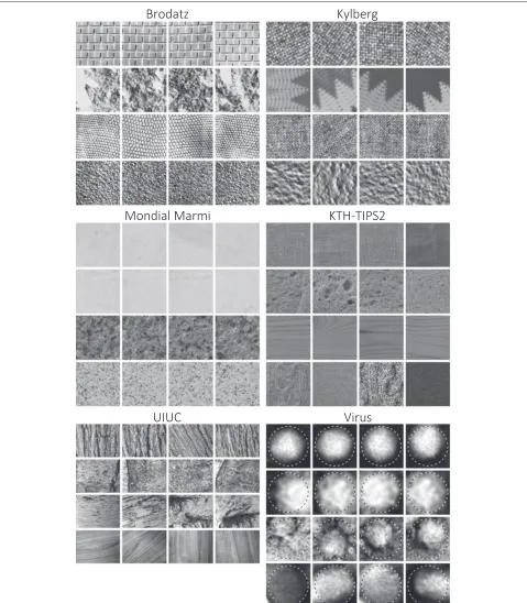
scale, perspective, and illumination. The texture datasets are Brodatz [13], KTH-TIPS2b [14], Kylberg [15], Mondial Marmi [16], UIUC [17], and a Virus texture dataset [11]. Figure 1 shows four samples from four classes in each of the six datasets. The basic properties of the datasets as well as links to websites where they are accessible are listed in Table 1.
The Brodatz dataset consists of digitized photographs of natural and manmade textures. In the form the Bro-datz photos are used here the dataset has many, 111, classes but only very few, 9, relatively homogeneous sam-ples per class. The samsam-ples are 213×213 pixels in size and there is a considerable overlap between a few of the classes making them indistinguishable. Some classes also include large structures making the nine samples not equally representative.
The KTH-TIPS2b dataset has 11 classes, some very het-erogeneous, with 432 samples each. In each class, four objects have been imaged under varying scale, illumina-tion, and pose conditions. For example, in the class “wool” four different fabrics and knitwear are represented which make this class very heterogeneous not only due to the varying imaging conditions. Most samples are 200×200 pixels in size, but some are smaller due to scale issues. See the documentation in [19] for details. In contrast to [14] where the dataset is used to study recognition of mate-rial categories we will use images from all four matemate-rial samples as examples of the same class when training the classifier.
The Kylberg dataset has 28 classes of 160 samples each with gray-scale images of different natural and manmade textured surfaces. The classes are very homogeneous in terms of perspective, scale, and illumination. The images in the Kylberg dataset are available in different rotations θ ∈ {0, 16π,26π,. . .,116π}. In this article, one orienta-tion per image is randomly selected. The 576×576 pixels images are here divided into four 288×288 pixels, non-overlapping, sub images resulting in 640 samples of each class.
The Mondial Marmi dataset is a collection of images of granite surfaces acquired as JPEG color images (with noticeable compression artifacts) under controlled illu-mination conditions. The dataset was used in [21] to evaluate robustness to rotation for LBP, coordinated clus-ters representation, and ILBP. While the texture samples are available in nine orientations (both hardware and soft-ware rotated) only one orientation (0◦) is used here. The 544 × 544 pixel images in the Mondial Marmi dataset are divided into four 272×272 pixel, non-overlapping, sub images. The samples are converted to gray scale as 0.2989 R+0.5870 G+0.1140 B, where R, G, and B are the red, green, and blue intensities, respectively.
Figure 1Texture examples.For each dataset four texture samples from four classes are shown. For the Virus dataset a dashed circle shows the perimeter of the region wherein the texture descriptors are computed.
images and appear to have only very minor compres-sion artifacts. Each class contains 40 samples (640 × 480 pixels) of different perspectives and scales of a texture.
Table 1 Properties of the six datasets used; references to the datasets are included
Dataset Number of Number of Total number of Sample Format Ref. Web link
classes samples samples size [px]
per class
Brodatz 111 9 999 213×213 GIF [13] [18]
KTH-TIPS2b 11 432 4752 200×200b PNG [14] [19]
Kylberga 28 640 17,920 288×288 PNG [15] [20]
Mondial Marmia 12 16 192 272×272 JPEG [21] [22]
UIUC 25 40 1,000 640×480 JPEG [17] [23]
Virus 15 100 1,500 41×41 PNG [11] [24]
aEach original sample is divided into four samples. bSome samples are smaller than 200×200 pixels.
The Virus dataset was first used in [11], and is based on transmission electron microscopy images of 15 dif-ferent virus types. The virus types vary both in size (diameters from 25 to 270 nm) and shape; some are icosa-hedral while others are elongated. Texture patches are extracted as disk-shaped regions with the same diame-ter as the viruses, cendiame-tered in automatically (not always correctly) segmented virus particles, see [11] for more details. The texture samples are then resampled to the same size (41×41 pixels) using a Lanczos kernel with a sinc window ofa=2. This disk-shaped region is shown in Figure 1.
3 Methods
In the original description of LBP [6], a window of 3× 3 pixels is used. The pixels in the window are compared to the value of the center pixel. By codingand<for each comparison as a binary number the local binary code is retrieved when reading these binary numbers anticlock-wise as a sequence, see Figure 2(left). The histogram of occurring binary codes in a region is the resulting fea-ture vector for that region. Early on, the definition was generalized to consider N sample points evenly dis-tributed on a circle with radius R from the cen-ter pixel [25], as illustrated in Figure 2(right). To make the comparison in this article as fair as pos-sible, the same generalization (using N samples on a radius R) is introduced for the whole LBP fam-ily of descriptors. The implementations of all the LBP family of descriptors are based on the original LBP implementation by Heikkilä and Ahonen accessible at [26].
To put the performance of the LBP family of descriptors into perspective, two other well-known texture descrip-tors are evaluated on the same datasets. The selected reference descriptors are Gabor filter banks (GF) and commonly used descriptors derived from the GLCM, also known as Haralick features. Table 2 lists all the descriptors in the comparison.
3.1 LBPs
The generalized LBP definition from [25] is used withN
sample points evenly distributed on a radiusRaround a center pixelpclocated at(xc,yc). The position,(xp,yp), of
the neighbor pointp, wherep∈ {0,. . .,N−1}is given by (xp,yp)=(xc+Rcos(2πp/N), yc−Rsin(2πp/N)).
(1)
The local binary code for the position(xc,yc)is defined as:
LBPN,R(x,y)= N−1
p=0
s(gp−gc)2p, (2)
where
s(x)=
1, x≥0
0, otherwise . (3)
If a pointpdoes not coincide with a pixel center, bilinear interpolation is used to compute the gray valuegp. Finally,
the histogram of occurring binary codes in a region is the feature vector of this region.
1
2
3
4
5
6
7
8
4
1
5
6
8
7
3
2
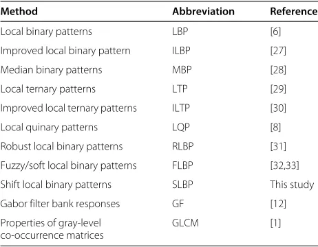
Table 2 Evaluated texture descriptors with abbreviations and references
Method Abbreviation References
Local binary patterns LBP [6]
Improved local binary pattern ILBP [27]
Median binary patterns MBP [28]
Local ternary patterns LTP [29]
Improved local ternary patterns ILTP [30]
Local quinary patterns LQP [8]
Robust local binary patterns RLBP [31] Fuzzy/soft local binary patterns FLBP [32,33] Shift local binary patterns SLBP This study
Gabor filter bank responses GF [12]
Properties of gray-level co-occurrence matrices
GLCM [1]
3.2 ILBPs
ILBP, introduced in [27], is closely related to LBP. The main difference is that the threshold used is the mean value of the whole neighborhood including the center pixel. In addition,pcwill also be a part of the binary code
making itN+1-bits long. Following [27], ILBP is defined as
ILBPN,R(x,y)= N−1
p=0
s(gp−gmean)2p+s(gc−gmean)2N, (4)
where
gmean= 1
N+1
⎛ ⎝N−1
p=0
gp+gc ⎞
⎠, (5)
and the functionsis defined as in Equation 3.
3.3 MBPs
MBP was introduced in [28]. In analogy to ILBP, the cen-ter pixelpcis included in the neighborhood but here the
median gray value of the neighborhood is used instead, giving the following definition:
MBPN,R(x,y)= N−1
p=0
s(gp−gmed)2p+s(gc−gmed)2N, (6)
where
gmed=median
{g0, g1,. . .,gN−1,gc} , (7)
and the functionsis defined as in Equation 3.
3.4 LTPs
To deal with the noise sensitivity of the LBP descriptor, the magnitude of the intensity difference between the center pixel and neighboring points can be taken into consider-ation. However, involving the magnitude implies that the complete invariance to intensity scaling is lost. In [29], the LTP descriptor is proposed. Here, the difference between neighboring values gp and the center pixel value gc are
encoded with three values using one thresholdt1 LTPN,R(x,y)=
N−1
p=0
s3(gp,gc,t1)2p, (8) where
s3(gp,gc,t1)=
⎧ ⎨ ⎩
1, gp≥gc+t1
0, gc−t1≤gp<gc+t1 −1, otherwise
. (9)
Instead of using a code with base 3 to encode the three states, LTP uses two binary codes representing the posi-tive and the negaposi-tive components of the ternary code, i.e., two binary codes coding for the two states{−1, 1}. These binary codes are collected in two separate histograms and, as a last step, the histograms are concatenated to form the LTP feature vector.
3.5 ILTPs
In analogy with the extension of LBP to ILBP, where the neighborhood mean value is used as the local thresh-old, LTP can be extended to ILTP. This was done in [30] arriving at the following definition:
ILTPN,R(x,y)= N−1
p=0
s3(gp−gmean)2p+s3(gc−gmean)2N, (10)
where the functions3is defined as in Equation 9 andgmean as in Equation 5.
3.6 LQP
In [8], LQP is introduced, extending the encoding of the local differences to five values corresponding to two thresholdst1andt2resulting in
LQPN,R(x,y)=
N−1
p=0
s5(gp,gc,t1,t2)2p, (11) where the two thresholds are used in the s5-function according to
s5(gp, gc, t1t2)=
⎧ ⎪ ⎪ ⎪ ⎪ ⎨ ⎪ ⎪ ⎪ ⎪ ⎩
2,gp≥gc+t2
1,gc+t1≤gp<gc+t2 0,gc−t1≤gp<gc+t1 −1,gc−t2≤gp<gc−t1 −2, otherwise
In analogy to LTP, the quinary code is split into four binary codes, coding for the states{−2,−1, 1, 2}. Four histograms are computed followed by a concatenation.
3.7 RLBP
By changing the expression (gp − gc) in Equation 2 to
(gp − gc − t1) the gray value in point p has to be t1 higher thangcto produce a 1. This modification is called
RLBPs and was introduced in [31]. The RLBP descriptor is supposed to improve robustness against small changes in local intensities. Following the description above, RLBP for a position(x,y)and a threshold valuet1is defined as
RLBPN,R(x,y,t1)= N−1
p=0
s(gp−gc−t1)2p, (13)
where the functionsis defined as in Equation 3.
3.8 FLBP
In fuzzy [32]/soft [33] LBP (FLBP) one pixel position may contribute to several bins in the histogram of possible pat-terns. A membership function for a neighboring pointp
to a ‘0-class’,m0, and the antonym functionm1, expressing belongingness to a ‘1-class’ is defined as
m0(p,f)=
⎧ ⎪ ⎨ ⎪ ⎩
0, gp≥gc+f f−gp+gc
2·f , gc−f ≤gp<gc+f
1, otherwise
, (14)
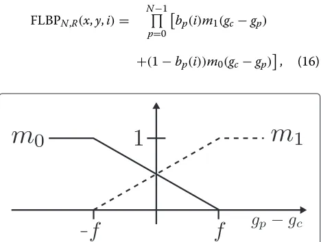
m1(p,f)=1−m0(p), (15) where f governs the interval of fuzzy belongingness. Figure 3 shows a plot of functionm0 andm1. The con-tribution from one pixel position (x,y)to a bini in the histogramHof occurring binary patterns is
FLBPN,R(x,y,i)= N−1
p=0
bp(i)m1(gc−gp)
+(1−bp(i))m0(gc−gp)
, (16)
Figure 3Membership functions in FLBP.The two membership functions used in FLBP. The gray value differencegp−gcon the
x-axis and belongingness on they-axis.
where bp(i) ∈ {0, 1} is the value of the pth bit of the
binary representation of patterni. By remembering that all considered pixel positions may contribute to biniin the histogram it follows that
HFLBP(i)=
x,y
FLBPN,R(x,y,i). (17)
Analogous to the other LBP-based descriptors, the result-ing histogram constitutes the FLBP feature vector.
3.9 SLBP
In the classical LBP definition, one pixel position gener-ates one local binary code corresponding to exactly one bin in the histogram of possible codes. In SLBP, a fixed number of local binary codes are generated for each pixel position. In analogy with RLBP the sign of an expression (gp−gc−k)is considered rather than the sign of(gp−gc)
as in the original LBP (Equation 2). However, in SLBP,k
is varied within an interval defined by an intensity limitl. Each timekis changed, a new binary code is created and added to the histogram of occurring binary patterns. SLBP for a position(x,y)and a shift valuekis defined as
SLBPN,R(x,y,k)= N−1
p=0
s(gp−gc−k)2p, (18)
where the functionsis defined as in Equation 3, andkis defined as
k∈[−l, l]∩Z. (19) The number of generated binary patterns,K, for one pixel position equals the number of different valueskassumes. From this and Equation 19 it follows that
K=2·l+1. (20) As an example, ifl =3, the parameterkwill assume val-ues{−3,−2,. . ., 3}.K will hence be 7 which means that each pixel position will contribute with 7 binary codes to the histogram. For neighborhoods with high local con-trast, the K binary codes may all be the same, while neighborhoods with contrast lower thanlwill generate a distribution of binary codes picking up some of the fuzzy nature of that neighborhood. The values in the final his-togram are divided by K, giving the histogram the sum equal to the number of pixel positions considered (like the rest of the LBP-family).
3.10 Rotation invariance of the LBP-family
are made rotation invariant in this way. LTP, ILTP, and LQP are somewhat different due to the concatenation of binary codes. The binary codes are therefore made rota-tion invariant prior to concatenarota-tion of the histograms here.
3.11 Gabor filters
In 1978, Granlund [12] generalized Gabor filters to 2D and applied them to images. In this article, the definition of the 2D Gabor filter in the spatial domain,ψ, is defined as in [35]
ψ (x,y,F,θ,γ,η)= F
2
π γ ηexp
−F2(x/γ )2+(y/η)2 ×expi2πFx ,
(21)
where
x=xcosθ+ysinθ, (22)
y= −xsinθ+ycosθ. (23)
Fis the frequency of the wave, andθis the angle between the direction of the wave and thex-axis. The Gaussian envelope is defined by the standard deviation parallel to the wave,γ, and standard deviation perpendicular to the wave,η.
A set of Gabor filters with different orientations and frequencies is commonly called a GF. Bianconi and Fernandez [35] show that parameters with a significant´ impact on the texture classification using GF are the fre-quency ratio and the standard deviations for the Gaussian envelope. They also conclude that a small change of a reasonable number of orientations,nO, or number of
fre-quencies,nF, in a GF does not significantly influence the
discriminating power for the texture datasets they con-sider. Based on their findings, a GF with a frequency ratio
equal to√2 is used here. The highest central frequency,
FM, is computed according to [35] as
FM =
γ
2(γ +(log 2/π )), (24)
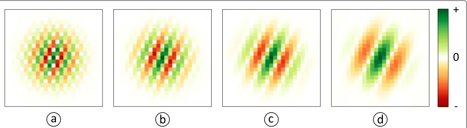
whereγ is the standard deviation of the Gaussian enve-lope parallel to the wave. Figure 4 shows an example of four Gabor filter kernels of the orientationθ =π/7 using γ =4,η=4⇒FM 0.53 and a frequency ratio of√(2).
When the GF descriptor is applied to a texture sam-ple the texture is convolved with the comsam-plex conjugate of each one of the constructed filters in the filter bank. The mean, μ, and standard deviation, σ, are computed for the magnitude of each filter response and these val-ues are used as the feature valval-ues. This results in a feature vector withnO×nF ×2 elements on the following form
GF= {μ00,σ00, μ01,σ01,. . .,μnO−1,nF−1,σnO−1,nF−1}.
(25)
Rotation invariance is achieved through the procedure proposed in [36]; for each frequency the dominant direc-tion is computed as the orientadirec-tion giving the highest mean filter response among the filters with this frequency in the filter bank. The elements in the GF feature vector are then circularly shifted so thatμandσ of the domi-nant direction can be found on the same positions in the feature vector. In [36], it is shown that a rotation of an image in the spatial domain corresponds to a circular shift of feature vector elements.
3.12 Gray-level co-occurrence matrices
Introduced in 1973 by Haralick et al. [1], descriptors derived from gray-level co-occurrence matrices still have a given place among established texture features. A relation operator is defined describing the distance and direc-tion between pixels whose intensities are to be pairwise
compared in the region of interest. A relation operator can, e.g., be ‘one pixel to the right’ and the following co-occurrence matrix, M, will then show how often a cer-tain gray value occurs one pixel to the right of another gray value. The gray levels of an image are commonly quantized into a lower number of intensity levels prior to computing the co-occurrence matrix. Quantization into q gray levels is used in this article resulting in a
q×qco-occurrence matrix of the gray levels defined as
M= ⎡ ⎢ ⎢ ⎢ ⎣
p(1, 1) p(1, 2) · · · p(1,q)
p(2, 1) p(2, 2) · · · p(2,q) ..
. ... . .. ...
p(q, 1) p(q, 2) · · · p(q,q)
⎤ ⎥ ⎥ ⎥
⎦, (26)
wherep(i,j)is the probability of the co-occurrence of the gray levelsi andjgiven a relation operator. In this arti-cle, the four symmetric relation operators
proposed by Haralick et al. is used. From the co-occurrence matrices, the contrast, correlation, energy, and homogeneity descriptors are computed as follows:
contrast=
i,j
|i−j|2p(i,j), (27)
correlation=
i,j
(i−μi)(j−μj)p(i,j)
σiσj , (28)
energy=
i,j
p(i,j)2, (29)
homogeneity=
i,j
p(i,j)
1+ |i−j|, (30)
where μi andμj are mean values computed along rows and columns, respectively. In the same way,σiandσjare standard deviations computed along rows and columns.
For each of the four descriptors, the average and stan-dard deviation over the four relation operators (direc-tions) are used as feature values. This results in a GLCM feature vector with eight elements. To fully describe the GLCM descriptor, the distancedin the relation operator also needs to be set.
3.13 Classification method
To get comparable noise robustness results and parameter optimization for the descriptors, a 1-NN with Euclidean metric is used. Tenfolded cross-validation is used to min-imize overfitting and to ensure that the validation is per-formed on independent test sets and the cross-validation is done by randomly assigning each sample a number
n∈ {1, 2,. . ., 10}, creating ten disjoint subsets with equal (or approximately equal) number of samples. In the first cross-validation fold, samples withn= 1 will be the test
data and samples withn∈ {2, 3,. . ., 10}will serve as train-ing data. In the second fold, samples withn=2 will be the test data and the rest is used for training, and so on. This means that each sample will be included in the test data once and less biased classification accuracy is obtained compared to using the apparent error. The ten results from the folds are combined into a single estimation.
The cross-validation folds are created once for each dataset and are then kept fixed throughout the compari-son. The feature values for all descriptors are normalized to [ 0, 1] prior to the cross-validation.
3.14 Parameter optimization
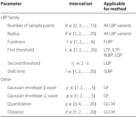
The parameters for each texture descriptor are optimized separately for each dataset to make as fair comparison as possible. The parameters common for all descriptors in the LBP family are the number of samplesN and the radiusR. Besides ILBP and MBP all extensions to the clas-sic LBP have additional parameters. The parameters are listed in Table 3 along with the range wherein they are varied. Since several parameters are common to several descriptors, the table also shows for which method each parameter is applicable.
To restrict the parameter search space, an optimization scheme is designed as follows:
1. Find optimalN and R for LBP using a tenfold cross-validated 1-NN classifier.
2. UseN and R from step 1 and find optimal: (a) fuzziness,f, for FLBP,
(b) thresholdt1for LTP, ILTP, and RLBP,
(c) threshold pairst1andt2for LQP, and
(d) interval limitl for SLBP. 3. For all texture descriptors
Perform a new gradient descent parameter search locally around the previous found best point in the current descriptor’s full
parameter space. Repeat until stability.
In other words, an exhaustive search for the best LBP parameters is performed. The LBP parameter val-ues are then used when optimizing all the method-specific parameters. They are next used as a starting guess for an iterative optimization procedure based on gradi-ent descgradi-ent where all parameters in the descriptors are allowed to vary.
The described optimization scheme is applied to each dataset separately. An exhaustive search for each of the parameters is not feasible due to the size of the datasets and total number of parameters across the descriptors.
Table 3 Descriptor parameters and the intervals searched during parameter optimization
Parameter Interval/set Applicable
for method LBP family
Number of sample points N∈ {2, 3,. . ., 15} All LBP variants Radius R∈ {1, 2,. . ., 20} All LBP variants Fuzziness f∈ {1, 2,. . ., 6} FLBP First threshold t1∈ {1, 2,. . ., 20} LTP, ILTP,
RLBP, LQP Second threshold t2=2·t1 LQP Shift limit l= {1, 2,. . ., 20} SLBP Other
Gaussian envelopewave γ∈ {1, 2,. . ., 5} GF Gaussian envelope⊥wave η∈ {1, 2,. . ., 5} GF Quantization q∈ {3, 4,. . ., 20} GLCM Distance d∈ {1, 2,. . ., 20} GLCM
3.15 Introducing noise
When the descriptor parameters have been optimized for each dataset the influence of noise is investigated. The noise model used is additive white (uncorrelated) Gaus-sian noise. That is, a sample from an GausGaus-sian distribution is added to the intensity of each pixel. This noise model is well suited for modeling thermal noise in CCD and CMOS sensors which are the sensors relevant for the microscopy and photography datasets considered here. The σ for the Gaussian distribution is gradually increased. Figure 5 shows one texture sample from each dataset under three different noise levels. The noise is added to the original datasets, and the noisy datasets are then saved. In this way, all the descriptors are applied and evaluated on the exact same noisy texture samples. The 20 noise levels used areσ from 10−4to 101with linearly spaced exponents, i.e., the 20 noise levels are equally spaced in a log10scale.
4 Results
4.1 Parameter optimization
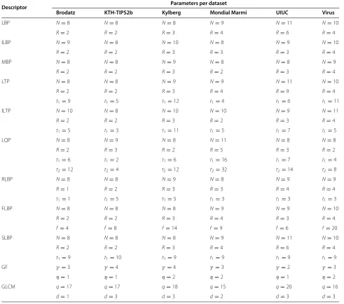
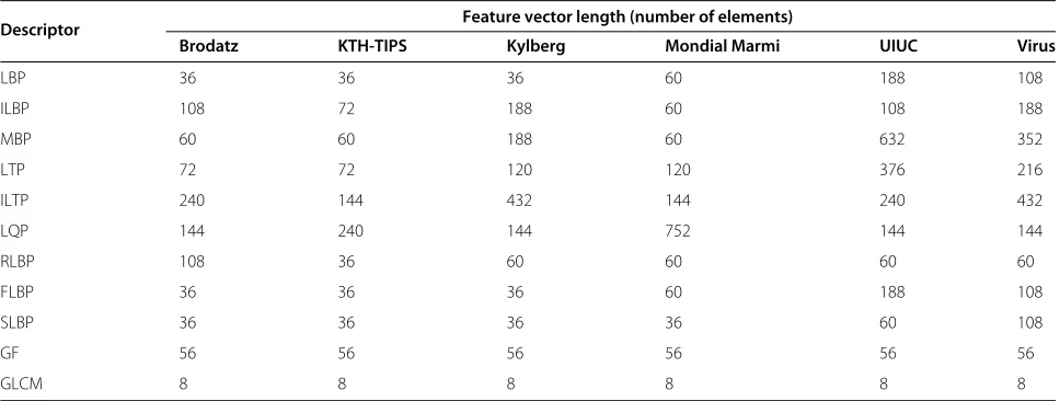
Table 4 lists the parameter values for each descriptor and dataset after applying the optimization scheme described in Section 3.14. The parameter choice does not only influ-ence the discriminant power of the descriptor but may also, depending on the descriptor, set the number of ele-ments in the feature vector. In the LBP family of descrip-tors, the feature vector length depends on the number of samplesNand whether or not the center pixel is included in the binary code. Table 5 lists the feature vector lengths for the descriptors after the parameter optimization.
4.2 Comparison without added noise
The discriminating power of the descriptors are compared on the datasets without added noise by analyzing the
combined classification accuracy of the tenfolded cross-validation. The classification accuracy may vary between datasets and descriptors, but also within a dataset for a specific descriptor, i.e., all classes may not equally be easy or difficult to discriminate. To explore this perspective, Figure 6 shows the distribution of mean accuracy per class for each descriptor and dataset.
Figure 6 shows that almost all descriptors perform well on the Kylberg dataset. LTP and ILTP manage to differ-entiate almost all classes perfectly in the Kylberg dataset (median very close to 100%, small boxes, and short tails). Most descriptors also perform well on the KTH-TIPS2b dataset. Even for the many classes in the Brodatz dataset all LBP descriptors perform overall well (100% for more than half the classes and boxes starting at > 88%) but there are a number of classes no method can discrimi-nate between (lowest class accuracies are between 22 and 44.4%). This is not surprising since there is a consider-able overlap between some of the classes in the Brodatz dataset, as mentioned before.
The other three datasets are more problematic with more varied results for the LBP descriptors. The overall low accuracies achieved on the Virus dataset are probably due to the small sample size (only 41×41 pixels), as well as the heterogeneous classes originating from the automatic extraction of patches only partly (or sometimes even not at all) containing virus. Across these three datasets, ILTP performs overall well as does FLBP.
GLCM is among the worst performing descriptors for all datasets, except for the Mondial Marmi dataset. Note however that only very few measures on the co-occurrence matrix are extracted.
The GF descriptor performs on the same level as several LBP-based descriptors for several datasets. However, on the Kylberg and UIUC dataset GF is outperformed by most LBP-based descriptors. Compar-isons of per-class performance for the different descrip-tors and datasets (data not shown) show that the GF sometimes produces good results for a few specific classes where the LBP family of descriptors do not. This indicates that GF could be a good complemen-tary texture descriptor and that a combination with, for example, ILTP might improve the overall classification accuracy on some of the datasets. However, combining descriptors to produce the best classification result pos-sible is not the purpose of this article, and is not further investigated here.
4.3 Robustness to noise
Table 4 Parameter settings for each descriptor and dataset after applied optimization scheme
Descriptor Parameters per dataset
Brodatz KTH-TIPS2b Kylberg Mondial Marmi UIUC Virus
LBP N=8 N=8 N=8 N=9 N=11 N=10
R=2 R=2 R=3 R=4 R=6 R=4
ILBP N=9 N=8 N=10 N=8 N=9 N=10
R=2 R=2 R=3 R=3 R=3 R=4
MBP N=8 N=8 N=9 N=8 N=8 N=9
R=2 R=2 R=3 R=2 R=3 R=4
LTP N=8 N=8 N=9 N=9 N=11 N=10
R=2 R=2 R=3 R=4 R=9 R=4
t1=9 t1=5 t1=12 t1=4 t1=6 t1=11
ILTP N=10 N=8 N=10 N=10 N=9 N=11
R=2 R=2 R=3 R=2 R=3 R=4
t1=5 t1=3 t1=11 t1=5 t1=7 t1=5
LQP N=8 N=9 N=8 N=11 N=8 N=8
R=2 R=3 R=2 R=5 R=3 R=2
t1=6 t1=2 t1=6 t1=16 t1=7 t1=4
t2=12 t2=4 t2=12 t2=32 t2=14 t2=8
RLBP N=8 N=8 N=9 N=8 N=9 N=9
R=1 R=2 R=3 R=3 R=4 R=4
t1=1 t1=5 t1=5 t1=3 t1=3 t1=3
FLBP N=8 N=8 N=8 N=9 N=9 N=10
R=2 R=2 R=3 R=4 R=3 R=4
f=4 f=8 f=14 f=9 f=6 f=20
SLBP N=8 N=8 N=8 N=9 N=11 N=10
R=2 R=2 R=3 R=4 R=6 R=4
t1=9 t1=10 t1=9 t1=9 t1=9 t1=9
GF γ=3 γ=4 γ =4 γ=3 γ =2 γ =3
η=1 η=1 η=2 η=2 η=1 η=2
GLCM q=17 q=17 q=18 q=15 q=20 q=16
d=1 d=3 d=3 d=2 d=3 d=3
in black. A horizontal dotted line marks the mean accu-racy of a random decision. The curves are interpolated between data points using piecewise cubic interpolation. For increasing noise levels, it is expected that the perfor-mance of all descriptors level out to the mean accuracy of a random classification, i.e., a mean classification accuracy of 1/number of classes. This is easily seen in, for example, Figure 9. The same data as Figures 7, 8, 9, 10, 11, and 12 show can be viewed in tabular form in Tables 6, 7, 8, 9, 10, and 11 but limited to every second noise level. In the tables, the highest mean accuracy for each noise level is highlighted in bold and the lowest in italics.
For the Brodatz dataset, Figure 7 and Table 6, GF stands out as the most noise robust texture descriptor but it is not
necessarily the best descriptor for low noise levels where ILTP followed by LTP, and SLBP show good performance. These four descriptors are better than LBP for all noise levels. RLBP, LQP, and especially MBP all perform worse than LBP, and in addition, the performance for LQP and MBP drops quickly with increasing levels of noise.
For low levels of noise in the KTH-TIPS2b dataset, Figure 8, all LBP-based descriptors (except MBP) outper-form the original LBP and they peroutper-form on the same high level as GF. For medium to high levels of noise all LBP-based methods are outperformed by GF and the bottom two LBP-based descriptors are, again, LQP and MBP.
Table 5 Feature vector length for each descriptor and dataset based on the optimized descriptor parameters
Descriptor Feature vector length (number of elements)
Brodatz KTH-TIPS Kylberg Mondial Marmi UIUC Virus
LBP 36 36 36 60 188 108
ILBP 108 72 188 60 108 188
MBP 60 60 188 60 632 352
LTP 72 72 120 120 376 216
ILTP 240 144 432 144 240 432
LQP 144 240 144 752 144 144
RLBP 108 36 60 60 60 60
FLBP 36 36 36 60 188 108
SLBP 36 36 36 36 60 108
GF 56 56 56 56 56 56
GLCM 8 8 8 8 8 8
ILTP are generally somewhat better than LBP. LQP drops in performance faster than the rest. The MBP perfor-mance drops with increasing but still low levels of noise, but then increases in performance and is among the bet-ter descriptors for high levels of noise. A closer look at the per-class accuracies (data not shown) reveals that it is mainly the second texture class, see Figure 1, with large
homogeneous intensity patches in the pattern that causes this dip in the mean accuracy curve for MBP.
For the Mondial Marmi dataset, Figure 8 and Table 9, the curves look and behave rather differently. A reason behind this might be the JPEG compression artifacts. This dataset is the only dataset where GLCM perform well for low levels of noise. GF is also found to perform well for
Figure 7Noise tests on Brodatz.Mean classification accuracy for all descriptors on the Brodatz dataset.
Figure 8Noise tests on KTH-TIPS2.Mean classification accuracy for all descriptors on the KTH-TIPS2 dataset.
Figure 10Noise tests on Mondial Marmi.Mean classification accuracy for all descriptors on the Mondial Marmi dataset.
low noise levels and is more stable than the other descrip-tors for increasing noise levels. ILBP, ILTP, and FLBP are generally better than LBP. However, for low levels of noise all the descriptors in the LBP family are similar, MBP and LBP being the exceptions. MBP is the worst performing descriptor as soon as low levels of noise are added and the performance of LQP drops quickly for higher levels of noise added.
On the UIUC dataset, LTP is the best performing descriptor for low levels of noise and ILTP and FLBP are in general better than the LBP, see Figure 11 and Table 10. GF is not very good for low to moderate noise levels but robust for high levels of noise. ILBP performs poorly for low levels of noise. MBP is the by far the worst performing descriptor followed by GLCM. Again, LQP drop quickly at moderate levels of noise and is hence less noise robust then the other LBP family of descriptors.
On the difficult Virus texture dataset, GF, ILTP, and FLBP are the best performing descriptors with FLBP hav-ing a slight upper hand at low levels of noise, see Figure 12 and Table 11. On this dataset, the proposed SLBP descrip-tor falls between these three best performing descripdescrip-tors and the rest while MBP and LQP are the two worst.
4.4 Computation time
One of the benefits of the classic LBP is that it is very fast to compute. A comparison of computation times for the more complex LBP descriptors is hence interesting. Computation time for some of the descriptors depend on the image content. Therefore, the CPU time required for the different descriptors is here compared on one sample from each class in the Kylberg dataset using the optimized parameters listed in Table 4. Figure 13 shows computa-tion time relative to the computacomputa-tion time of the classic LBP. Hence, if a descriptor takes 10 times longer than LBP
Table 6 Mean classification accuracy for descriptors computed on the Brodatz dataset
Brodatz dataset
σof noise 0 0.0002 0.0006 0.0021 0.0070 0.0234 0.0785 0.2637 0.8859 2.9764 10.0000
LBP 92.8 91.2 89.9 87.7 83.5 78.9 64.4 38.2 13.5 4.5 2.9
ILBP 94.2 93.9 92.5 90.7 88.8 80.0 71.8 50.8 27.6 12.5 6.2
MBP 92.5 80.6 69.0 57.9 45.9 28.0 23.6 15.2 12.2 5.2 3.7
LTP 96.6 94.8 94.7 91.8 87.9 81.4 68.1 43.0 20.8 8.7 4.3
ILTP 96.4 96.2 95.2 94.3 91.4 85.7 70.7 50.7 28.5 10.9 4.2
LQP 93.7 91.6 91.1 82.8 62.6 43.7 36.2 21.5 8.6 3.6 3.7
RLBP 89.4 86.6 89.0 82.9 77.9 70.6 51.6 26.8 11.7 4.5 2.6
FLBP 92.6 91.6 91.5 89.5 85.5 79.8 65.5 36.6 12.7 5.0 4.5
SLBP 93.9 93.0 92.4 91.1 88.2 83.4 68.8 39.3 17.2 6.4 3.0
GF 87.2 86.8 87.0 86.7 86.0 85.3 81.2 70.9 34.5 7.7 1.2
GLCM 83.2 81.3 80.6 79.8 75.2 64.7 49.8 34.6 13.8 4.0 0.9
Table 7 Mean classification accuracy for descriptors computed on the KTH-TIPS2b dataset
KTH-TIPS2b dataset
Noise levels 0 0.0002 0.0006 0.0021 0.0070 0.0234 0.0785 0.2637 0.8859 2.9764 10.0000
LBP 89.3 87.2 86.1 80.4 68.5 53.1 43.7 29.4 23.3 18.9 14.9
ILBP 94.5 94.4 93.6 87.4 74.1 59.2 47.4 38.4 27.7 21.8 17.4
MBP 94.1 84.3 73.6 60.2 48.0 40.4 35.4 28.9 23.2 17.5 14.6
LTP 95.5 94.7 93.2 87.2 71.5 55.4 44.1 32.1 25.3 19.5 16.2
ILTP 96.9 96.4 95.7 90.8 79.4 65.4 50.6 39.2 28.0 22.4 17.6
LQP 94.8 93.6 87.2 70.0 57.2 46.5 38.7 27.9 20.3 18.1 14.7
RLBP 93.8 92.7 90.6 83.7 69.9 53.0 42.4 30.4 23.0 19.3 16.0
FLBP 94.3 94.0 93.1 88.6 74.9 56.9 44.2 29.8 21.9 18.2 15.7
SLBP 94.8 94.5 93.5 89.2 76.6 57.8 44.1 30.1 22.8 18.5 16.2
GF 94.6 94.7 94.1 93.8 90.8 83.9 66.4 41.3 22.3 12.9 10.1
GLCM 76.9 76.2 76.0 73.9 71.7 62.5 54.0 39.5 25.0 18.7 12.7
Max value per noise level is in bold and min value in italics.
to compute the descriptor has the value 10 in the plot in Figure 13.
Furthermore, two FLBP implementations are compared. The version directly based on [32,33], called ‘naive’ in Figure 13, computes the histogram bin contribution of all bins for every neighborhood (Equation 16). However, gray value differences outside the fuzzy region [−f, f] restrict the possible binary codes that a neighborhood can contribute to. Utilizing this, a modified implementation was developed, denoted ‘fast’ in Figure 13. It restricts the membership computations to the subset of binary codes possible, given the current local neighborhood. Outside the fuzzy region, the bin contributions will be as in the classic LBP. The computed feature vectors from the ‘naive’ and ‘fast’ implementations of FLBP are of course identical.
Even though the ‘fast’ FLBP implementation is roughly five times faster than the ‘naive’ implementation, they are both very slow compared to all other descriptors. FLBP are 922 times slower than the classic LBP. It should also be said that the computation time for the ‘fast’ FLBP not only depends on the fuzziness parameter (which is the case of the ‘naive’ FLBP), but also depends on the image content. Figure 13 shows that LQP, RLBP, ILTP, LTP, ILBP, and GLCM have comparable computation times to LBP. SLBP is roughly 11 times slower than LBP which is expected since SLBP in this test generates 11 binary codes at every position (l = 5 ⇒ K = 11, see Equation 20). The MBP is relatively slow compared to most of the LBP descriptors which is also expected since computing median values in this implementation involves sorting the intensity values in each neighborhood. In GF, which is 20
Table 8 Mean classification accuracy for descriptors computed on the Kylberg dataset
Kylberg dataset
Noise levels 0 0.0002 0.0006 0.0021 0.0070 0.0234 0.0785 0.2637 0.8859 2.9764 10.0000
LBP 97.8 97.5 97.0 95.6 89.2 70.3 44.0 22.4 9.2 5.4 5.1
ILBP 98.9 98.6 98.2 96.4 91.1 76.0 53.8 35.3 16.4 8.2 5.9
MBP 96.8 91.3 84.5 80.9 85.7 80.3 57.0 26.2 7.1 4.1 3.2
LTP 99.7 99.6 99.5 98.5 94.1 80.6 52.5 25.3 9.9 6.3 4.9
ILTP 99.7 99.6 99.4 99.0 97.2 86.1 65.1 41.1 18.0 8.3 5.4
LQP 99.3 98.5 98.1 93.7 72.1 41.3 23.9 13.8 6.3 4.6 4.2
RLBP 98.8 98.6 98.1 96.1 91.0 75.1 46.9 21.1 7.4 5.3 4.3
FLBP 99.2 99.4 99.4 99.0 95.4 76.6 45.2 22.3 8.2 4.8 4.5
SLBP 98.0 98.1 97.7 95.5 87.7 65.7 38.4 19.2 8.2 5.1 4.4
GF 95.2 94.7 94.0 92.8 89.7 78.7 58.5 32.6 11.5 4.3 3.7
GLCM 84.7 84.8 85.1 84.4 79.8 63.1 51.8 31.0 12.2 4.9 3.5
Table 9 Mean classification accuracy for descriptors computed on the Mondial Marmi dataset
Mondial Marmi dataset
Noise levels 0 0.0002 0.0006 0.0021 0.0070 0.0234 0.0785 0.2637 0.8859 2.9764 10.0000
LBP 85.9 80.2 78.1 80.7 60.9 52.1 52.1 33.9 24.0 20.8 22.4
ILBP 95.8 93.2 95.8 83.3 66.7 54.2 67.2 61.5 50.0 55.2 39.6
MBP 90.1 82.8 64.6 40.6 29.2 28.1 17.7 16.7 35.9 32.3 25.0
LTP 94.8 88.5 88.5 79.2 69.8 55.7 57.3 39.6 37.5 27.6 24.0
ILTP 93.8 91.1 88.5 88.0 70.8 62.5 71.4 55.2 40.6 46.9 29.2
LQP 89.6 89.6 88.5 88.0 59.9 31.8 37.0 23.4 28.1 25.5 20.8
RLBP 85.9 86.5 90.1 77.6 65.6 51.6 46.9 41.7 35.9 33.9 22.9
FLBP 95.3 94.3 91.7 81.3 68.8 56.3 61.5 33.9 22.4 22.9 15.6
SLBP 91.1 93.2 90.1 83.3 67.2 45.8 57.3 47.9 33.3 24.0 26.0
GF 94.8 94.8 94.3 93.2 90.1 81.3 75.5 37.0 25.5 10.9 8.9
GLCM 95.8 91.7 90.6 89.1 77.6 61.5 51.0 52.6 26.0 10.9 9.9
Max value per noise level is in bold and min value in italics.
times slower than LBP, each texture sample is convolved with a number of complex filter kernels. This is a more time-consuming task than performing multiple threshold-ings in a small neighborhood, the operation performed in most LBP-based descriptors.
5 Conclusions
This article reports on the following:
• The descriptive performance of eight LBP-based texture descriptors are evaluated and compared on six different datasets under increasing levels of additive Gaussian white noise together with the classic LBP, Haralick descriptors, and GF.
• A new LBP-based descriptor, SLBP, is introduced as a fast approximation of the computationally heavy FLBP.
• A roughly five times faster implementation of the FLBP descriptor is described.
The fast implementation of FLBP as well as an implemen-tation of SLBP are available as Matlab code at [37].
The main conclusions that can be drawn regarding the evaluated texture descriptors are
• ILTP followed by FLBP generally perform well among the LBP-family of descriptors, outperforming the classic LBP in all tests performed.
• GF is often very robust for moderate to high levels of noise but is many times outperformed by several LBP-based descriptors under low noise conditions.
• FLBP is very slow compared to the rest of the descriptors but the naive implementation can be
Table 10 Mean classification accuracy for descriptors computed on the UIUC dataset
UIUC dataset
Noise levels 0 0.0002 0.0006 0.0021 0.0070 0.0234 0.0785 0.2637 0.8859 2.9764 10.0000
LBP 88.1 87.2 87.5 88.6 86.4 75.8 53.8 38.4 22.3 12.5 9.4
ILBP 80.1 80.8 79.6 80.6 74.8 63.5 59.4 53.4 37.9 25.7 17.8
MBP 74.7 63.7 56.9 47.1 39.3 27.1 14.1 15.3 14.3 13.7 13.3
LTP 94.4 94.1 93.8 93.4 88.1 77.9 59.5 44.6 23.8 16.5 13.7
ILTP 91.9 91.5 91.9 90.4 85.1 72.9 64.2 55.6 42.7 24.7 17.9
LQP 88.3 86.5 82.8 75.1 49.4 36.0 38.7 37.7 23.2 15.4 12.3
RLBP 89.4 89.0 90.4 87.7 84.7 72.0 56.3 38.7 26.7 16.8 14.2
FLBP 91.3 91.5 91.1 90.3 87.5 79.2 64.3 43.3 22.4 13.5 12.2
SLBP 87.3 87.2 88.9 91.2 86.7 78.5 65.3 43.3 25.5 16.4 12.8
GF 74.2 74.1 74.2 74.4 74.5 71.4 67.4 58.9 36.5 18.4 9.4
GLCM 62.3 60.8 59.8 57.0 55.2 49.0 48.0 34.2 18.4 11.4 4.4
Table 11 Mean classification accuracy for descriptors computed on the Virus dataset
Virus dataset
Noise levels 0 0.0002 0.0006 0.0021 0.0070 0.0234 0.0785 0.2637 0.8859 2.9764 10.0000
LBP 40.3 40.1 37.7 34.5 26.9 17.3 13.9 10.0 7.5 7.2 7.7
ILBP 38.1 37.1 35.4 34.1 27.2 22.0 18.4 13.9 11.0 10.7 6.5
MBP 37.3 32.1 30.6 30.9 25.1 21.7 17.9 12.9 9.1 7.1 4.9
LTP 48.2 44.8 42.7 36.8 30.4 22.1 13.9 11.9 8.8 7.0 7.4
ILTP 53.1 51.5 49.2 43.9 36.9 29.0 20.2 14.5 10.5 8.4 6.8
LQP 39.1 36.1 33.3 27.7 19.7 12.1 13.1 11.8 9.5 7.8 7.7
RLBP 40.7 37.1 34.7 31.5 27.8 19.7 14.8 9.3 9.5 8.0 7.5
FLBP 54.5 53.8 50.3 47.7 36.8 24.3 16.4 10.6 7.0 8.3 7.0
SLBP 47.0 46.7 42.7 41.1 30.9 20.0 14.0 9.4 6.7 7.3 7.1
GF 51.6 51.5 49.2 46.9 35.7 27.1 15.0 10.3 7.7 7.6 5.7
GLCM 40.4 38.6 38.7 37.9 31.6 24.9 20.1 12.6 9.9 6.7 6.9
Max value per noise level is in bold and min value in italics.
improved upon by restricting the belongingness computations to the possible subset of binary codes given a specific neighborhood.
• MBP is very noise sensitive and has a relatively poor performance even for low levels of noise.
• LQP suffer more of added noise than the majority of the LBP-based descriptors.
• It is not possible to know in advance which texture descriptor is the best performing one for a given problem. However, a well-performing descriptor can probably be found among a subset of the tested descriptors, after optimizing their parameters. Such a subset of descriptors could be ILBP, LTP, ILTP, and FLBP. Furthermore, SLBP can sometimes be an alternative to the computationally heavy FLBP.
In accordance with the survey in [9], ILTP is found to be superior to LTP, LQP, and ILBP for all the datasets
evaluated. In addition, we show that ILTP retains its dis-crimination advantage under increasing levels of added Gaussian white noise. The results presented here also show that even if MBP and LQP perform relatively well on noise free data, they both suffer greatly from the intro-duced noise. Furthermore, we find that FLBP has a good overall performance, similar to ILTP.
It seems that it is preferable to use the more stable local mean value of the neighborhood (including the center pixel) as the local threshold in that ILBP often outper-forms LBP, and ILTP often outperoutper-forms LTP. The two descriptors using ternary patterns, LTP and ILTP, often outperform their counterparts using binary codes, the LBP and ILBP descriptors, suggesting that the use of ternary patterns has its advantage.
The two descriptors MBP and LQP are often found among the worst performing descriptors both regarding overall accuracy and robustness to noise. The reason for
Figure 12Noise tests on Virus.Mean classification accuracy for all descriptors on the Virus dataset.
the poor performance of MBP can be explained by its definition. Using the median value as the local threshold results in that half of the gray levels in the neighborhood will be larger and half smaller. This restricts the possible binary codes, and as a consequent, restricts the amount of discriminative information that can be contained in the MBP descriptor.
GF involves convolution with relatively large (between 13×13 and 25×25 pixels) complex filter kernels and is hence slow in comparison to most of the other descrip-tors, proves to be a very noise robust descriptor for all datasets but not always among the best performing descriptors at low noise levels.
Under increasing levels of noise the discriminating power of the descriptors is expected to drop monoton-ically, or at least close to monotonically. This holds for most tests reported on here except for the results for the Mondial Marmi dataset which are somewhat odd, see
Figure 8. While the mean classification accuracies have a decreasing trend, the curves are far from monotonically decreasing. One possible cause may be the JPEG com-pression artifacts present in this dataset. The blocking artifacts from the 8×8 blocks used in JPEG compression are at a scale comparable to that of the local neighbor-hoods used in the LBP family. As expected, GF, with its larger considered regions, shows a smoother decline under increasing levels of noise.
A comparison of the per-class performance and confu-sion matrices for the descriptors at a few noise levels has been done (data not shown). The LBP family of descrip-tors tend to have difficulties with mostly the same classes (MBP and LQP have additional difficulties). The per-class accuracy for GF and the LBP descriptors is often similar even though the LBP descriptors are more alike among themselves (apart from MBP). This is in line with the find-ings reported in [38]. The per-class accuracy for GLCM
differs from those of the LBP family and GF mainly in that GLCM has additional difficulties discriminating a number of classes. FLBP has a high over all accuracy but with a slightly different pattern in the per-class accuracy compared to the rest of the LBP-family on the Brodatz, Kylberg, and Virus datasets. Similarly, GF has a slightly different distribution of per-class accuracy than the LBP-family on the Brodatz, KTH-TIPS2b, and Mondial Marmi datasets.
A different distribution of per-class accuracy indicates that the descriptors compared detect different charac-teristics of the textures. On some datasets used here a combination of ILTP or FLBP and GF could presumably be beneficial for the task of texture classification. However, combining texture descriptors to improve classification accuracy is not within the scope of this article.
In parallel with the 1-NN classifier used in the results reported in this article, SVMs were also investigated on the datasets without added noise using both a linear and a Gaussian kernel with optimized parameters. Similar descriptor parameter values were suggested by the SVM classifiers in the optimization procedure for the texture descriptors. For some dataset–descriptor combinations, the SVMs reached slightly higher classification accura-cies. Nevertheless the 1-NN classifier was used in the tests reported on to make the comparison between the descriptors on the same and fair basis.
Competing interests
The authors declare that they have no competing interests.
Acknowledgments
The authors would like to thank Vladimir ´Curi´c for his input on notations. Some of the computations were performed on resources provided by SNIC through Uppsala Multidisciplinary Center for Advanced Computational Science (UPPMAX) under Project p2012012. This study is part of the MiniTEM E!6143 project funded by EU and EUREKA through the Eurostars Programme.
Author details
1Centre for Image Analysis, Uppsala University, Uppsala, Sweden.2Centre for
Image Analysis, Swedish University of Agricultural Sciences, Uppsala, Sweden.
Received: 1 October 2012 Accepted: 20 March 2013 Published: 15 April 2013
References
1. RM Haralick, K Shanmugam, I Dinstein, Textural features for image classification. IEEE Trans. Syst. Man Cybern.3(6), 610–621 (1973) 2. A Jain, Learning texture discrimination masks. IEEE Trans. Pattern Anal.
Mach. Intell.18(2), 195–205 (1996)
3. M Pietikäinen, A Hadid, G Zhao, T Ahonen,Computer Vision Using Local Binary Patterns, vol. 40 of Computational Imaging and Vision.
(Springer, London, 2011)
4. D Harwood, T Ojala, M Pietikäinen, S Kelman, L Davis,
Texture classification by center-symmetric auto-correlation, using Kullback discrimination of distributions. Pattern Recognit. Lett.
16, 1–10 (1995)
5. L Wang, DC He, Texture classification using texture spectrum. Pattern Recognit.23(8), 905–910 (1990)
6. T Ojala, M Pietikäinen, D Harwood, A comparative study of texture measures with classification based on featured distributions. Pattern Recognit.29, 51–59 (1996)
7. L Nanni, A Lumini, S Brahnam, Survey on LBP based texture descriptors for image classification. Expert Syst. Appl.39(3), 3634–3641 (2012) 8. L Nanni, A Lumini, S Brahnam, Local binary patterns variants as texture
descriptors for medical image analysis. Artif. Intell. Med.49(2), 117–125 (2010)
9. A Fernández, M Álvarez, F Bianconi, Texture description through histograms of equivalent patterns. J. Math. Imag. Vision.
45, 76–102 (2013)
10. T Mäenpää, T Ojala, M Pietikäinen, M Soriano, inProceedings 15th International Conference on Pattern Recognition, ICPR 2000,
vol. 3. Robust texture classification by subsets of local binary patterns (Barcelona, Spain, 2000), pp. 935–938
11. G Kylberg, M Uppström, IM Sintorn, inProceedings of the 16th Iberoamerican Congress on Pattern Recognition, CIARP 2011, vol. 7042 of Lecture Notes in Computer Science. Virus texture analysis using local binary patterns and radial density profiles (Pucón, Chile, 2011), pp. 573–580 12. GH Granlund, In search of a general picture processing operator.
Comput. Graph. Image Process.8(2), 155–173 (1978)
13. P Brodatz,Textures: A Photographic Album for Artists and Designers. (Dover Publications, New York, 1966)
14. B Caputo, E Hayman, P Mallikarjuna, inProceedings of the 10th IEEE International Conference on Computer Vision, ICCV 2005, vol. 2.
Class-specific material categorisation (Beijing China, 2005), pp. 1597–1604 15. G Kylberg,The Kylberg Texture Dataset v. 1.0. External report (Blue series) 35,
Centre for Image Analysis, Swedish University of Agricultural Sciences and Uppsala University, (Uppsala, Sweden, 2011). http://www.cb.uu.se/~ gustaf/texture/
16. A Fernández, MX Álvarez, F Bianconi, Image classification with binary gradient contours. Opt. Lasers Eng.49(9–10), 1177–1184 (2011) 17. S Lazebnik, C Schmid, J Ponce, A sparse texture representation using local
affine regions. IEEE Trans. Pattern Anal. Mach. Intell.
27(8), 1265–1278 (2005)
18. T Randen, Brodatz textures at Trygve Randen’s website (2011). http:// www.ux.uis.no/~tranden/
19. KTH-TIPS 2b (2012). http://www.nada.kth.se/cvap/databases/kth-tips/ 20. G Kylberg. Kylberg Texture Dataset v.1.0 (2012). http://www.cb.uu.se/~
gustaf/texture/
21. A Fernández, O Ghita, E González, F Bianconi, PF Whelan, Evaluation of robustness against rotation of LBP , CCR and ILBP features in granite texture classification. Mach. Vis. Appl.22(6), 913–926 (2010) 22. Mondial Marmi Texture Dataset v. 1.1 (2012). http://dismac.dii.unipg.it/
mm/ver_1_1/
23. UIUC Texture Database (2012). http://www-cvr.ai.uiuc.edu/ponce_grp/ data/
24. G Kylberg, Virus Texture Dataset v. 1.0 (2012). http://www.cb.uu.se/~ gustaf/virustexture/
25. T Ojala, T Mäenpää, Multiresolution gray-scale and rotation invariant texture classification with local binary patterns. IEEE Trans. Pattern Mach. Intell.24(7), 971–987 (2002)
26. M Heikkilä, T Ahonen, (2012). http://www.cse.oulu.fi/CMV/Downloads/ LBPMatlab
27. H Jin, Q Liu, H Lu, X Tong, inProceedings of the 3rd International Conference on Image and Graphics, ICIG 2004. Face detection using improved LBP under Bayesian framework (Hong Kong China, 2004), pp. 306–309 28. A Hafiane, G Seetharaman, B Zavidovique, inProceedings of the 4th
International Conference, ICIAR 2007, vol. 4633 of Lecture Notes in Computer Science. Median binary pattern for textures classification (Montreal, Canada, 2007), pp. 387–398
29. X Tan, B Triggs, Enhanced local texture feature sets for face recognition under difficult lighting conditions. IEEE Trans. Image Process.
19(6), 1635–1650 (2007)
31. M Heikkilä, M Pietikäinen, A texture-based method for modeling the background and detecting moving objects. IEEE Trans. Pattern Anal. Mach. Intell.28(4), 657–662 (2006)
32. DK Iakovidis, EG Keramidas, D Maroulis, inProceedings of the 5th International Conference on Image Analysis and Recognition, ICIAR 2008, vol. 5112 of Lecture Notes in Computer Science. Fuzzy local binary patterns for ultrasound texture characterization (Póvoa de Varzim Portugal, 2008), pp. 750–759
33. T Ahonen, M Pietikäinen, inProceedings of the Finnish Signal Processing Symposium, FINSIG 2007, vol. 1. Soft histograms for local binary patterns (Oulu, Finland, 2007), pp. 1–4
34. N Herve, A Servais, E Thervet, JC Olivo-Marin, V Meas-Yedid, inProceedings of the IEEE International Symposium on Biomedical Imaging: From Nano to Macro, ISBI 2011. Statistical color texture descriptors for histological images analysis (Chicago, USA, 2011), pp. 724–727
35. F Bianconi, A Fernández, Evaluation of the effects of Gabor filter parameters on texture classification. Pattern Recognit.40(12), 3325–3335 (2007)
36. D Zhang, A Wong, M Indrawan, G Lu, inProceedings of the First IEEE Pacific-Rim Conference on Multimedia, PCM 2000. Content-based image retrieval using Gabor texture features (Sydney, Australia, 2000), pp. 1139–1142
37. G Kylberg, FLBP and SLBP implementations for Matlab (2013). http:// www.cb.uu.se/~gustaf/textureDescriptors/
38. O Ghita, D Ilea, A Fernandez, P Whelan, Local binary patterns versus signal processing texture analysis: a study from a performance evaluation perspective. Sensor Rev.32(2), 149–162 (2012)
doi:10.1186/1687-5281-2013-17
Cite this article as:Kylberg and Sintorn:Evaluation of noise robustness for
local binary pattern descriptors in texture classification.EURASIP Journal on Image and Video Processing20132013:17.
Submit your manuscript to a
journal and benefi t from:
7Convenient online submission
7 Rigorous peer review
7Immediate publication on acceptance
7 Open access: articles freely available online
7High visibility within the fi eld
7 Retaining the copyright to your article