Statistical Averaging Method and New Statistical Averaging Method for Solving Extreme Point Multi–Objective Linear Programming Problem

(1)

doi: 10.11648/j.ml.20180403.12

ISSN: 2575-503X (Print); ISSN: 2575-5056 (Online)

Statistical Averaging Method and New Statistical Averaging

Method for Solving Extreme Point Multi–Objective Linear

Programming Problem

Samsun Nahar

1, *

, Samima Akther

2

, Mohammad Abdul Alim

3 1_{Department of Basic Sciences & Humanities, University of Asia Pacific, Dhaka, Bangladesh} 2

Department of Mathematics, University of Barisal, Barisal, Bangladesh 3

Department of Mathematics, Bangladesh University of Engineering & Technology, Dhaka, Bangladesh

Email address:

*

Corresponding author

To cite this article:

Samsun Nahar, Samima Akther, Mohammad Abdul Alim. Statistical Averaging Method and New Statistical Averaging Method for Solving Extreme Point Multi–Objective Linear Programming Problem. Mathematics Letters. Vol. 4, No. 3, 2018, pp. 44-50.

doi: 10.11648/j.ml.20180403.12

Received: October 2, 2018; Accepted: October 16, 2018; Published: November 14, 2018

Abstract:

In this paper, statistical averaging method (arithmetic mean, geometric mean) and new statistical averaging method (new arithmetic mean, new geometric mean) have been proposed for extreme point multi-objective linear programming problem (EPMOLPP). Extreme point can be taken from graphical representation of linear programming problem (LPP). Graphical solution of LPP has been discussed in this research The objective of this method is for making single objective from multi-objective extreme point linear programming problem. Chandra Sen’s method is for making single objective from multi-objective linear programming problem (MOLPP). Here Chandra Sen’s method has also been used to solve EPMOLPP. An algorithm and program solution have been given for our proposed method to solve such type of problems. A numerical example is given and the result in Table 2 indicates that the proposed technique gives better results.

Keywords:

Extreme Point Linear Programming Problem, Statistical Averaging Method, New Statistical Averaging Method, Extreme Point Multi-Objective Linear Programming Problem (EPMOLPP)

1. Introduction

Multi-objective programming is used in application for many real world problems including problems in the fields of engineering, mining and finance. In multi-objective programming there are multiple conflicting objectives whereby improving one objective will reduce the value of others, leading to a trade-off between solutions. It is assumed that no single solution will optimize all objectives simultaneously because this would be a trivial case.

The main aim of multi-objective programming is to assist a decision maker (DM) to choose a preferred solution among all the trade-offs. In this case, it is not necessary to generate all solutions when the DM is involved in the process since some solutions may be eliminated at each stage.

In the last few decades multi–objective linear

programming problem has become an interesting field for some researcher and the achievement is remarkable in the respective research area. A lot of important works have been done such as, Abdul-Kadir and Sulaiman [1] proposed an approach for multi-objective fractional programming problem. Sulaiman and Mustafa [2] discussed harmonic mean to solve multi-objective linear programming problems. Nahar and Alim [3] generalized multi-objective linear fractional programming problem by a new geometric average method to get optimal solution.

(2)

A discussion has been given by Abdulrahim [5] about Extreme Point Quadratic Fractional Programming Problem (EPQFPP). Nawkhass [6] has developed wolfes method and

modified simplex method for Quadratic fractional

programming problem (QFPP). Weighed sum method for MOLPP has been discussed by Nahar and Alim [7]. A new statistical averaging method for MOLPP has been proposed by Nahar and Alim [8]. Geometric average technique to solve Extreme Point Multi- Objective Quadratic Programming Problems (EPMOQPP) has been given by Sulaiman et al. [9]. Hossain et al. [10] proved an alternative approach for solving extreme point linear fractional programming problem. Among them, Sulaiman [11] discussed the computational aspects of single-objective indefinite quadratic programming problem with extreme point. Hamad-Amin [12] used average technique to solve an extreme point complementary multi-objective linear programming problem (EPCMOLPP).

In this paper an EPMOLPP is defined and statistical averaging method (arithmetic, geometric mean) and new statistical averaging method (new arithmetic, new geometric mean) have been proposed for EPMOLPP. New statistical averaging method gives better result than statistical averaging method.

2. Extreme Point Linear Programming

Problem

Extreme point linear programming problem was formulated by Kirby et al. [13] as follows:

Max (Min)Z =CX

subject to:AX ≤b

where X is an extreme point of

0

DX d X

≤ ≥

where C is n -dimensional vector of constants; X isn

-dimensional vector of variables. A is m × n matrix of

constants; b ism-dimensional vector of constants. D is p × n -matrix of constants and d is p × 1vector of constants.

Extreme point multi-objective linear programming problem can be defined as follows:

1 1 1

2 2 2

1 1 1

t

r r r

t

r r r

t

s s s

Maxz C x r Maxz C x r

Maxz C x r Minz C x r

Minz C x r

+ + +

= +

⋯⋯⋯⋯⋯⋯⋯

(1)

subject to:

AX b ≤

   

=

   _≥  

(2)

where X is an extreme point of

0

DX d X

≤

≥ (3)

wherer is the number of objective functions to be maximized,

s is the number of objective functions to be maximized and minimized, (s-r)is the number of objective functions to be

minimized, X is an n -dimensional vector of decision

variables, C is an n-dimensional vector of constants and

r , i = 1,2, … … s are scalar constants.

3. Methodologies to Solve EPMOLPP

3.1. Chandra Sen’s Method

The combined objective function of Chandra Sen's technique in Sen [14] can be shown in equation

1| | 1| |

r s

i i

i i r

z z

Max z

φ φ

= = +

=

∑

−

∑

(4)

and can be solved it by simplex method with the same constraints (2) and (3).

Suppose that it can be obtained a single value corresponding to each of the objective function of the EPMOLPP of equation (1) subject to the constraints (2) and (3) as in equation

1 1

2 2

1 1

...

r r

s s Max z Max z

Max z Min z

Min z φ

φ

φ φ

φ

+ +

= =

=

(5)

where φ , (i = 1,2, … … , s) are the values of objective

functions.

3.2. Algorithm of Chandra Sen’s Technique

An algorithm for obtaining the optimal solution for the EPMOLPP can be summarized as follows:

Step 1: Find values of each of the individual objective function which is to be maximized or minimized.

Step 2: Solve the first objective function by simplex method with constraints.

Step 3: Check the feasibility of the solution in step 2, if it is feasible then go to step 4, otherwise, use dual simplex method to remove infeasibility.

(3)

objective function to Maxz called φ . Step 5: Repeat the step 2, i=1, 2,....,r

Step 6: Determine Chandra Sen’s technique.

Step 7: Optimize the combined objective function (4), under the same constraints (3), by repeating steps 2-4.

3.3. Proposed Statistical Averaging Technique

For making single objective function from multi-objective functions

1 1

. ( ) . ( )

r s

i i

i i r

r s

i i

i i r

z z

Max z

A M AA A M AL

z z

Max z

G M AA G M AL

= = +

= −

∑

where,AA_i =|φ_i|,i=1,⋯,randALi =|φi|i= +1 r,⋯,s

3.4. Proposed New Arithmetic Averaging Technique

Letm1=min AAi , whereAAi =|φi|,φiis maximum value

of zi, i=1,⋯,r

2 min i

m = AL _{, where}AL_i =|φ_i|,φiis minimum value of

i

z, i= +r 1,⋯,s

1 2

.

2

m m A Av= + so

1 1

/ .

r s

i i

i i r

Max z z z A Av

= = +

 

= − 

 



∑



(6)

3.5. Proposed New Geometric Averaging Technique

Using m1 and m2 obtained, it can be found the geometric

average as follows:

1 2

.

G Av= m m

1 1

/ .

r s

i i

i i r

Max z z z G Av

= = +

 

= − 

 



∑

 (7)

3.6. Algorithm for Proposed Method

Step 1: Graph the feasible region Step 2: Draw an isoprofit line

Step 3: Move parallel to the isoprofit line in the direction of increasing z. The last point in the feasible region that contacts an isoprofit line, is an optimal solution to the LP.

Step 4: Find the value of each of individual objective function which is to be maximized or minimized.

Step 5: Solve the problem with first objective function by simplex method.

Step 6: Check the feasibility of the solution in step 2. If it is feasible then go to step 4. Otherwise, use dual simplex method to remove infeasibility.

Step 7: Assign a name to the optimum value of the first

objective functionz1sayφ1.

Step 8: Repeat the step 2, i=1, 2, …, s

Step 9: Select m1=min AAi ,m2 =min ALi ,i=1,⋯,s

1 2

.

2

m m

A Av= + and G Av. = m m₁ ₂

Step 10: Optimize the combined objective function with the same constraints

1 1

/ .

r s

i i

i i r

Max z z z A Av

= = +

 

= − 

 



∑



1 1

/ .

r s

i i

i i r

Max z z z G Av

= = +

 

= − 

 



∑



subject to:

AX b ≤

   

=

   _≥  

where X is an extreme point of .

0

D X d X

≤ ≥

Step 11: Solve problem by simplex method.

3.7. Program Solution for Proposed Method

The following program can be used to solve EPMOLPP by the proposed method

For this, let

i A

φ = value of objective functions which is to be maximized.

i L

φ = value of objective functions which is to be minimized

so

| |

i i

AA =φA ;∀ i=1,⋯,r; ALi=|φLi|; ∀ i= +1 r,⋯,s

1 r

i i

SM z

= =

∑

;

1 s

i i r

SN z

= + =

∑

1 min i

m = AA ;m2 =min ALi

(

)

/ .

Max z= SM−SN A Av Max z=

(

SM−SN

)

/G Av.

subject to:

AX b

≤    ₌    _≥  

where X is an extreme point of .

0

D X d X

≤ ≥

(4)

4. Statistical Analysis

We construct numerical example to illustrate the technique for solving EPMOLPP

1 1

2 1 2

3 1 2

4 1 2

5 1 2

2

3 4

4 5

Max z x

Max z x x

Min z x x

= = − − = + = − − = − −

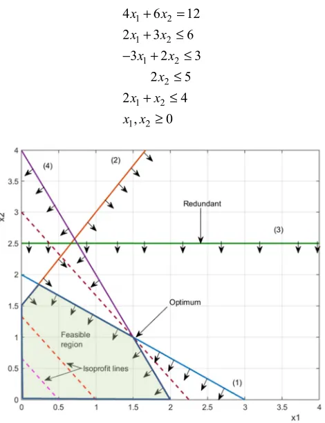
subject to 4x1+6x2=12

(x1, x2) is an extreme point of

1 2 1 2 2 1 2

1 2

2 3 6

3 2 3

2 5

2 4

, 0

x x x x x x x

x x

+ ≤ + ≤ ≤ + ≤

≥

4.1. Graphical Solution of LPP

The feasible region for any LP is a convex set, Sottiner [15]. If LP has an optimal solution, there is an extreme (or corner) point of the feasible region that is an optimal solution to the LP. We may graphically solve an LP (max problem) with two decision variables as follows:

Step 1: Graph the feasible region Step 2: Draw an isoprofit line

Step 3: Move parallel to the isoprofit line in the direction of increasing z. The last point in the feasible region that contacts an isoprofit line is an optimal solution to the LP.

4.2. Graphical Analysis of LPP

This section shows how to solve a two-variable linear programming problem graphically, which can be illustrated as follows:

Example: Consider Maximize Z =x1

subject to

1 2 1 2

2 1 2 1 2

2 3 6

3 2 3

2 5

2 4

, 0

x x x x

x x x x x

+ ≤ − + ≤

≤ + ≤

≥

For the first objective function, we get

Maximize Z1=x1

subject to

1 2

2 1 2 1 2

4 6 12

2 3 6

3 2 3

2 5

2 4

, 0

x x

x

x x

x x

+ = + ≤ − + ≤

≤ + ≤

≥

From simplex algorithm we get the optimal solution, x1=1.5, x2=1, Zmax=1.5

For the second objective function, we get

Maximize Z2=-x1-2x2

subject to

1 2

2

1 2

4 6 12

2 3 6

3 2 3

2 5

2 4

, 0

x x x x x x

x x x x x

+ =

+ ≤

− + ≤

≤ + ≤

≥

Figure 1. Graphical solution of LPP.

From simplex algorithm we get the optimal solution, x1=1.5, x2=1, Zmax=-3.5

For the third objective function, we get

Maximize Z3=3x1+4x2

subject to

1 2

2

1 2

4 6 12

2 3 6

3 2 3

2 5

2 4

, 0

x x x x x x

x x x x x

+ =

+ ≤

− + ≤

≤ + ≤

≥

For the forth objective function, we get

Maximize Z4=-3x1-4x2

(5)

1 2 1 2 1 2

2 1 2 1 2

4 6 12

2 3 6

3 2 3

2 5

2 4

, 0

x x

x

x x

x x

+ = + ≤ − + ≤

≤ + ≤

≥

From simplex algorithm we get the optimal solution, x1=1.5, x2=1, Zmin=-8.5

For the fifth objective function, we get

Maximize Z5=-4x1-5x2

subject to

1 2

2

1 2

4 6 12

2 3 6

3 2 3

2 5

2 4

, 0

x x x x x x

x x x x x

+ =

+ ≤

− + ≤

≤ + ≤

≥

From simplex algorithm we get the optimal solution, x1=1.5, x2=1, Zmin=-11

Thus

Table 1. Optimal table.

I φφφφi xi AAi=|φφφφi| ALi=|φφφφi|

1 1.5 (1.5, 1) 1.5

2 -3.5 (1.5, 1) 3.5

3 8.5 (1.5, 1) 8.5

4 -8.5 (1.5, 1) 8.5

5 -11 (1.5, 1) 11

By Chandra Sen’s technique,

Max Z=

1| | 1| |

r s

k k

k k r

z z

φ φ

= = +

−

∑

1 1 2 1 2

1 2 1 2

1 2

2 3 4

1.5 3.5 8.5

3 4 4 5

8.5 11

(0.67 0.286 0.353 0.353 0.364) ( 0.571 0.471 0.471 0.454) 1.101 0.825

x x x x x

Max Z

x x x x

x x

− − + = + + −

− − − −

 

+

 

 

= − + + + + − + + + = +

Thus we get a single objective function and our EPMOLPP becomes

Maximize Z=1.101x1+0.825x2

subject to

1 2 1 2 1 2

2 1 2 1 2

4 6 12

2 3 6

3 2 3

2 5

2 4

, 0

x x

x

x x

x x

+ = + ≤ − + ≤

≤ + ≤

≥

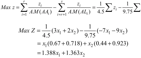
Using arithmetic averaging,

1.5 3.5 8.5

.. ( ) 4.5

3 8.5 11

.. ( ) 9.75

2

i

A M AA and

A M AL

+ +

= =

+

= =

1 1

. ( ) . ( ) 4.5 9.75

r s

i i

i i r

z z

Max z z z

A M AA A M AL

= = +

=

∑

−

∑

=

∑

−

∑

1 2 1 2

1 2

1 1

(3 2 ) ( 7 9 )

4.5 9.75

(0.67 0.718) (0.44 0.923)

1.388 1.363

Max Z x x x x

x x

= + − − −

= + + +

= +

subject to

1 2

2

1 2

4 6 12

2 3 6

3 2 3

2 5

2 4

, 0

x x x x x x

x x x x x

+ =

+ ≤

− + ≤

≤ + ≤

(6)

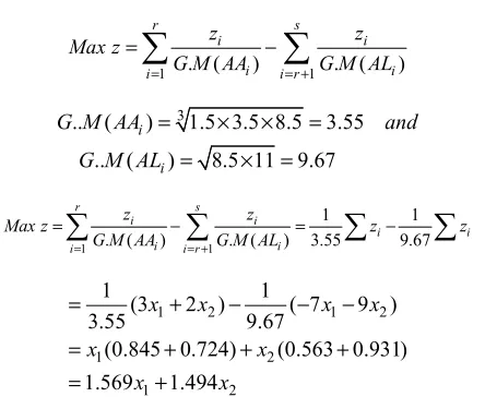
Using geometric averaging

1 . ( ) 1 . ( )

r s

i i

i i r

z z

Max z

G M AA G M AL

= = +

=

∑

−

∑

3

.. ( ) 1.5 3.5 8.5 3.55

.. ( ) 8.5 11 9.67

i

G M AA and

G M AL

= × × =

= × =

1 1

. ( ) . ( ) 3.55 9.67

r s

i i

i i r

z z

Max z z z

G M AA G M AL

= = +

=

∑

−

∑

=

∑

−

∑

1 2 1 2

1 2

1 1

(3 2 ) ( 7 9 )

3.55 9.67

(0.845 0.724) (0.563 0.931)

1.569 1.494

x x x x

x x

= + − − −

= + + +

= +

subject to

1 2

2

1 2

4 6 12

2 3 6

3 2 3

2 5

2 4

, 0

x x x x x x

x x x x x

+ =

+ ≤

− + ≤

≤ + ≤

≥

New arithmetic averaging technique:

Let m1=1.5, m2=8.5; 1 2 5

2

m +m ₌

1 1

/ .

r s

i i

i i r

Maxz z z A Av

= = +

 

= − 

 



∑



1 2 1 2 1 2

1

[3 2 7 9 ] 2 2.2

5 x x x x x x

= + + + = +

Maximize Z=2x1+2.2x2

subject to

1 2

2

1 2

4 6 12

2 3 6

3 2 3

2 5

2 4

, 0

x x

x x x x x

+ =

+ ≤

− + ≤

≤ + ≤

≥

New geometric averaging technique:

1 1

/ .

r s

i i

i i r

Maxz z z G Av

= = +

 

= − 

 



∑



1.5 8.5× =3.57

1 2 1 2

1

[10 11 ] 2.801 3.081

3.57

Maxz= x + x = x + x

subject to

1 2

2

1 2

4 6 12

2 3 6

3 2 3

2 5

2 4

, 0

x x

x x x x x

+ =

+ ≤

− + ≤

≤ + ≤

≥

5. Result and Discussion

In this paper, two techniques such as statistical averaging technique for EPMOLPP and new statistical averaging technique for EPMOLPP have been discussed and the results are compared in the following table. From table 2 it can be seen that geometric mean gives better result than arithmetic mean. Also geometric averaging gives better result than arithmetic averaging.

Table 2. Comparison between statistical and new statistical averaging technique.

Statistical averaging technique for EPMOLPP New statistical averaging technique for EPMOLPP

Using A. M Using G. M Using A. Av Using G. Av

(7)

6. Conclusion

From the above table it is apparent that new statistical averaging technique for EPMOLPP gives better result than statistical averaging technique for EPMOLPP. In the same time, it is also clear that in the proposed method results are increasing consistently.

Acknowledgements

I acknowledge the continuous support and comments received from Dr. Md. Abdul Alim.

References

[1] M. S. Abdul-Kadir and N. A. Sulaiman, “An approach for multi objective fractional programming problem”, Journal of the College of Education, University of Salahaddin, vol. 3. pp 1-5, 1993.

[2] N. A. Sulaiman and R. B. Mustafa, “Using harmonic mean to solve multi-objective linear programming problems”, American journal of operations Research, 6, 25-30, 2016. [3] S. Nahar and M. A. Alim, “A New Geometric Average

Technique to Solve Multi-Objective Linear Fractional Programming Problem and Comparison with New Arithmetic Average Technique”, IOSR Journal of Mathematics (IOSR-JM) e-ISSN: 2278-5728, p-ISSN: 2319-765X. vol. 13, issue 3 ver. 1, pp 39-52, DOI: 10.9790/5728-1303013952, 2017. [4] S. H. Frederick and J. L. Gerald, "introduction to operations

research" seventh edition published by McGraw-Hill, an imprint of The McGraw-Hill companies, inc., 1221, 2001. [5] B. K. Abdulrahim, “On Extreme Point Quadratic Fractional

Programming Problem” Applied Mathematical Sciences, Vol. 8, no. 6, 261 – 277, 2014.

[6] M. A. Nawkhass, “On Solving Quadratic Fractional Programming Problems” M. Sc. Thesis, Salahaddin university Erbil Iraq, 2014.

[7] S. Nahar and M. A. Alim , “Weighted Sum Method for Making Single Objective from Multi-objective Linear Programming Problem (MOLPP) and Comparison with Chandra Sen’s Method”, (accepted) BSME conference (BUET), 2018.

[8] S. Nahar and M. A. Alim, “A New Statistical Averaging Method to Solve Multi-Objective Linear Programming Problem, ” International Journal of Science and Research (IJSR), ISSN: 2319-7064, Vol. 6 No. 8, 2017.

[9] N. A. Sulaiman, R. M. Abdullah and S. O. Abdul, “Using Optimal Geometric Average Technique to Solve Extreme Point Multi- Objective Quadratic Programming Problems” Journal of Zankoi Sulaimani, Part- A. (Pure Applied Science), 2016.

[10] T. Hossain, M. R. Arefin and M. A. Islam, “An Alternative Approach for Solving Extreme Point Linear and Linear Fractional Programming Problem” Dhaka University. J. Sci. vol.63. no.2, pp 77-84, 2015.

[11] N. A. Sulaiman, “Extreme Point Quadratic Programming Techniques” M. Sc. Thesis, University of Salahaddin, Erbil/Iraq, 1989.

[12] A. O. Hamad-Amin, “An Adaptive Arithmetic Average Transformation Technique for Solving MOLPP”, M. Sc. Thesis, University of Koya, Koya/Iraq, 2008.

[13] M. J. L. Kirby, H. R. Love, and S. Kanti, “Cutting Plan Algorithm for Extreme Point Mathematical Programming", Cashier. Ducentre D Etudes De Recherche Operationelle, vol.14, no.1 pp 27-42, 1972.

[14] C. Sen, “A New Approach for Multi objective Rural Development Planning”, The Indian Economic Journal, vol.30, pp.91-96.