Estimating HIES Data through Ratio and Regression Methods for Different Sampling Designs

Regression Methods for Different Sampling Designs

Faqir Muhammad

Allama Iqbal Open University Islamabad

Ayesha Anis

Allama Iqbal Open University Islamabad

Abstract

In this study, comparison has been made for different sampling designs, using the HIES data of North West Frontier Province (NWFP) for 2001-02 and 1998-99 collected from the Federal Bureau of Statistics, Statistical Division, Government of Pakistan, Islamabad. The performance of the estimators has also been considered using bootstrap and Jacknife.

A two-stage stratified random sample design is adopted by HIES. In the first stage, enumeration blocks and villages are treated as the first stage Primary Sampling Units (PSU). The sample PSU’s are selected with probability proportional to size. Secondary Sampling Units (SSU) i.e., households are selected by systematic sampling with a random start.

They have used a single study variable. We have compared the HIES technique with some other designs, which are:

Stratified Simple Random Sampling. Stratified Systematic Sampling. Stratified Ranked Set Sampling. Stratified Two Phase Sampling.

Ratio and Regression methods were applied with two study variables, which are: Income (y) and

Household sizes (x). Jacknife and Bootstrap are used for variance replication.

Simple Random Sampling with sample size (462 to 561) gave moderate variances both by Jacknife and Bootstrap. By applying Systematic Sampling, we received moderate variance with sample size (467). In Jacknife with Systematic Sampling, we obtained variance of regression estimator greater than that of ratio estimator for a sample size (467 to 631). At a sample size (952) variance of ratio estimator gets greater than that of regression estimator. The most efficient design comes out to be Ranked set sampling compared with other designs. The Ranked set sampling with jackknife and bootstrap, gives minimum variance even with the smallest sample size (467). Two Phase sampling gave poor performance.

Multi-stage sampling applied by HIES gave large variances especially if used with a single study variable.

1. Introduction

the changes which occur, as a result of economic development in the consumption pattern, incidence of poverty, trend in the saving propensities and preferences of different groups of population. Moreover, the information on per capita income of the household sector may also be of use in evaluating the validity of the National Income estimates obtained through conventional methods. In Pakistan, the report on household income and consumption data is given by Household Integrated Economic Survey (HIES) and Pakistan Integrated Household Survey (PIHS). The HIES has seen some major developments during the 1990s. The Household integrated Economic Survey (HIES) was conducted, with some breaks, since 1963. In 1990 HIES questionnaires were revised in order to address the requirements of a new system of national accounts. The four surveys of 1990-91, 1993-94 and 1996-97 followed the design of these new questionnaires. In 1998, the HIES data collection methods and questionnaires were changed to reflect the integration of the HIES with the Pakistan Integrated Household Survey (PIHS).

The national average household size was 6.8 members in 1998, but it differs between rural and urban areas and provinces. Household size in Sindh is slightly larger than of Punjab. But household in NWFP and Baluchistan have approximately one more member than households in Punjab and Sindh. From the results of the last three surveys, the numbers of earners to the household has tended to increase in both urban and rural areas. The household size in 2001-02 has reached to 6.96 as described in HIES 2001-02.

HIES applies multistage stratified random sample design for estimation. During this study, we have compared different sampling techniques for estimating HIES data.

2. Methodology

In this study, HIES data is collected from the Statistical Division, Islamabad, of two years. It was used to develop ideas for future for Income and household size. Income groups with respect to household sizes of Pakistan and its provinces in (1998-1999) and (2001-2002) were taken and estimated where

x = Household size y = Income

2.1 Methods of Estimation

Occasions arise where the estimation of the population mean or total for a variable X is assisted by information on a subsidiary variable Y. Two ways to do this is by ratio or regression estimation

2.1.1 Ratio method - Stratified sample

As discussed by Yates (1981), each stratum is treated separately, using the formula for a random sample and build up the population estimates by summation of the estimates of separate strata, with division by N for population

means i.e.,

∑

⎥ ⎦ ⎤ ⎢ ⎣ ⎡ = i i i X x S y S Y ) ( ) (

ˆ _(2.1)

stratum each in x S y S r ) ( ) ( = (2.2)

{

}

{

}

∑

∑

− = ⎥ ⎦ ⎤ ⎢ ⎣ ⎡ − = 2 2 2 2 2 ) 1 ( ) 1 ( ) ( ) ( i q i q i i i s n f g s n f x S X y V i (2.3) 2 ) ( ) ( X y V r

V = (2.4)

Here the 2

i q

s are estimated separately for each stratum, using the value of the ratio appropriate to the stratum

1 2 − = i i i q n Q

s (2.5)

(

) (

)

{

}

2

∑

− − −

= i i i i i

i S y y r x x

Q (2.6)

2.1.2 Regression method – Stratified Sample

The linear regression estimator is more efficient than the ratio estimator except when the regression line of y on x passes through neighborhood of origin in which case the efficiency of these estimators is almost equal

)

(X x

b y

ylr = + − (2.7)

lr lr Ny

y = (2.8)

{

}

{

2

}

) ( ) )( ( x x S x x y y S b i i i i i − − − = (2.9)

The procedure the same in every strata

) )( (

)

( _{i i} 2 _{i i i i i i}

i

i S y y bS y y x x

Q =

∑

− −

∑

− − (2.10)

2 2 − = i i i q n Q

s (2.11)

{

}

∑

−

= 2 2

) 1 ( ) ( i q i

lr g f n s

y

V (2.12)

Where

X = Total of x for the population

y

N = Number of units in the population. Y = Total of y for the population. f = Sampling fraction

g = 1 / f

2.2 Sampling Techniques

Cochran (1977) has described that in stratified sampling the population of N units is first divided into subpopulations of N1, N2, ………..,NL units, respectively.

These subpopulations are non overlapping, and together they comprise the whole of the population, so that

N1 + N2+……..+NL = N

The subpopulations are called strata. To obtain the full benefit from stratification, the values of the Nh must be known. When the strata have been determined, a

sample is drawn from each, the drawings being made independently in different strata. The sample sizes within the strata are denoted by n1, n2,………., nL,

respectively.

As the data was in stratified form so we have used stratification in every technique.

2.2.1 Simple Random Sampling

As discussed by Thompson (1992), simple random sampling, is a method of selecting n units out of the N, such that, every one of the NCn distinctly sample

has an equal chance of being drawn. In practice, a simple random sample is drawn unit by unit either by means of a table of random numbers or by means a computer program that produces such a table.

The above procedure is used independently in each stratum to get the final results

In simple random sampling,

∑

=

= n i

i

n y y

1

(2.13)

The procedures of ratio and regression estimation are used after drawing the sample randomly.

2.2.2 Systematic Sampling

Sample obtained by randomly selecting one element from the first k elements in

the sampling frame, and every kth element thereafter, is called a 1-in-k

Systematic Sampling. For stratified systematic sampling, the same procedure is used for every stratum

In systematic sampling, for k possible systematic samples

Y y k y

k y

E sys = + + k =

1 .... 1

)

The estimates are calculated using the above ratio and regression methods after drawing the sample systematically.

2.2.3 Ranked Set Sampling

In Ranked Set Sampling, from a population of N elements, a sample of n

elements is drawn by simple random sampling. The drawing is repeated independently n times, so, we have n independent samples of size n each. Next,

we rank each sample. Then, choose for the final sample, the element with smallest ranked from the first sample, the element with the second smallest ranked from the second sample, and so on. Kowalczyk (2004) has written in detail about ranked set sampling.

The same procedure is used for every stratum

Elements y1(1:n), y2(2:n),… , yn(n:n) constitute the ranked set sample. The mean of

ranked set sample is denoted byyRSS.

∑

=

= n

i n i i

RSS y

n y

1 ) : ( 1

(2.15)

Then, the ratio and regression methods are applied.

2.2.4 Two Phase Sampling

A multi-phase sample collects basic information from a large sample of units and then, for a smaller sample, may be sub sample, collects more detailed information. The most common form of multi-phase sampling is two-phase sampling, but three or more phases are also possible.

Multi-phase sampling is useful when the frame lacks auxiliary information that could be used to stratify the population or to screen out part of the population. Multi-phase sampling is beneficial when there is insufficient budget to collect information from the whole sample, or when doing so would create excessive burden on the respondent, or even when there are very different costs of collection for different questions on a survey.

We used stratification in both phases. In ordinary stratification, we can use population values, in two phase sampling, we must use their estimates obtained in the preliminary sample of size m. Thus the estimate of mean, by Kish (1965),

is

h hy w

y=

∑

(2.16)

Where, w_h =m_h/m

The variance of the regression estimate, as discussed by Mukhopadhyay (1998), is approximately given by,

n S S m S lr

y x y x y

y

V

2 . 2 . 2

)

(

=

+

− (2.17)

⎥

⎦

⎤

⎢

⎣

⎡

−

−

−

=

∑

∑

= =

−

m

i

m

i

m i i

m x

y

y

y

b

x

x

S

1 1

2 2

2 2

1 . 2

)

(

)

Where

∑

= − −

=

m i m y y y i

S

1 1 ) ( 2 2

The variance of the ratio estimate is approximately given by

n x S R m x S R S R

S y yx

y

V

2 2

2 2 2 ˆ ˆ ˆ 2

)

(

=

− +

+

(2.19)

Where ) ( 1 2 1 ) ( 2 1

ˆ

1 ) ( 2 1 ) )( ( 1 ) ( 2 m m i i m m i m i i m i i x y m x x x m x x y y yx m y y

R

S

S

y

S

=

=

∑

=

∑

=

− ∑ − − − − − − = = =

Details are given in Sukhatme and Sukhatme (1984).

2.2.5 Two Stage Sampling

In multi-stage sampling a frame is required at each stage for the units that have been selected at that stage. Initially, a frame is taken by which first-stage units may be defined and selected. For the second-stage of selection, a frame is required by which second-stage units may be defined within the first-stage units which have been selected.

One of the advantages of multi-stage sampling is that second-stage frames are only required for selected first-stage units and so on.

According to Som (1973), the combined unbiased estimator of Yh from all the nh

FSU’s is the arithmetic mean

∑

= nh hi

h

ho y

n

y* 1 * (2.20)

With an unbiased variance estimator

∑

− − = h ho y n h h h

hi y n n

y

s2 ( * *₀)2/ ( 1)

* (2.21)

For the whole universe, an unbiased estimator of the total Y =

∑

L Y_h is

∑

= L y_ho

y * (2.22)

With an unbiased variance estimator

∑

= L _y

y s _ho

Table: Sampling plan for a stratified two-stage desing with pps sampling at the first-stage and sys or srs at the second-stage. In the hth stratum (h= 1, 2,……,L)

Stage t Unit No. in

universe

No. in sample

Selection method

Selection probability

ft

1 First-stage Nh nh Ppswr π_hi =Z_hi/Z_h nhπhi

2

Second-stage Mhi mhi

sys or srs

hi

M

Equal= 1 mhi/Mhi

An unbiased estimator of the hth stratum totalYh(h=1,2,...,L), obtained from the ith FSU (i=1,2,…….,nh) is

hi hi

hi m

j hij hi hi

hi

hi y

M y

m M y

hi

π

π =

=

∑

=1 *

(2.24)

Where y_hij is the value of the study variable in the jth selected SSU (household or

field) of the ith selected FSU (village) in the hth stratum, and

∑

=

= mhi j

hi hij

hi y m

y

1

/ (2.25)

In the mean of the y_hij values in the hith sample FSU.

The combined unbiased estimator of Yh is

∑

= nh _{hi h}

ho y n

y* * / (2.26)

And an unbiased estimator of the overall total Y is

∑

=

L

y

_ho

y

* (2.27)

2.3 The Replication methods for Variance Estimation

For variance replication, we have used 1) Jacknife and 2) Bootstrap.

2.3.1 Jacknife

The jackknife is a method in statistics allowing one to judge the uncertainties of estimators derived from small samples, without assumptions about the underlying probability distributions. The method consists of forming new samples by omitting, in turn, one of the observations of the original sample. For each of the samples thus generated, the estimator under study can be calculated, and the probability distribution thus obtained will allow one to draw conclusions about the estimator's sensitivity to individual observations. The procedure given by Chaudhuri and Stenger (1992) is given as;

In the Jacknife, we form n DELETE-1 sub-samples

θ

ˆ(i) by computing our

Jackknife estimate of standard error is

∑

=

− −

= n

i i jack

n n se

1

2 (.) )

( )

ˆ (

1 _{θ θ}

(2.28)

where

n n

i i

∑

=

= 1 () (.)

ˆ

ˆ θ

θ

For stratified sampling, jackknife is applied independently in each stratum by omitting one observation, out of the dataset, as given by Lohr (1999).

2.3.2 Bootstrapping

The bootstrap is a method to determine the trustworthiness of a statistic, comparable to the standard deviation of a mean. The bootstrap is a generalization of this standard deviation.

It is a re-sampling procedure to assess the accuracy of an estimator and is in fact computing power as a substitute for theoretical analysis. Shao and Tu (1995) have given following bootstrap algorithm;

We have pairs (yi, xi), i = 1,2,…,N where yi’s are random and xi’s fixed. We call

this regression experiment.

Assign equal probabilities to each yi for i = 1,2, … , N

Construct bootstrap sample * *

2 *

1 ,y ,....,yN

y as follows

i i

i y y

e = − ˆ , Where yˆ_i=αˆ+βˆx_i (2.29)

αˆand βˆare the values of regression parameters estimated from the regression

experiment.

*

* _ˆ

ˆ _{i i}

i x e

y =α+β + (2.30)

Where e*i is selected from e1, e2, …, eN using sampling with replacement with the

help of normal distribution.

Calculate C*, D* from the bootstrap sample (y*i, xi) i = 1,2,…,N using μ and σ2

calculated from the relation with B known.

Repeat 3rd step B times and calculate

B

C

C

ˆ

*

=

Σ

*j

/

j = 1, 2, ….,B (2.31)

B D

Dˆ* =Σ *j / (2.32)

B C

C C

R A

Vˆ (ˆ*)=[Σ( *_j − ˆ*)2}/ (2.33)

B D D D

R A

Vˆ (ˆ*)=[Σ( *_j− ˆ*)2}/ (2.34)

3. Results and Discussion

The data set of HIES collected from The Federal Bureau of Statistics, Islamabad was in SPSS format. From this data set, the data of NWFP province was extracted for further analysis. The data was in stratified form in 33 strata.

In MINITAB software a number of macros are developed for the calculations and results.

A sample size of approximately 25% of N was taken.

N = 1918

2.3.3 Simple Random Sampling

Stratified Simple Random Sampling was applied 50 times and obtained mean of means, and mean of variances and ratios. Stratified simple random sampling is a good selection for this data. It is small variance with Jacknife. But with bootstrap having sample size 462, the results gave smaller variance for ratio estimates compared to regression estimates which is not possible. A slightly bigger sample i.e., 561, gives the desired answers.

2.3.4 Systematic Sampling

Stratified Systematic Sampling is bad choice for HIES 2001-02 data. It gives large variances for regression estimates in comparison with ratio estimates with Jacknife. Only for a very large sample sizes, as 952, gives the appropriate answers. With Bootstrap, sample of 631 gives the appropriate results.

2.3.5 Ranked Set Sampling

It is the most efficient sampling technique for this data. For the sample size of 467, it gives minimum variances. It is also suitable with Jacknife and Bootstrap.

2.3.6 Two Phase Sampling

It gives large variances. With Bootstrap, for smaller sample sizes, with 1353 sample (HIES 1998-99) and sample of 544 (HIES 2001-02) gives the desired results. Jacknife performs poorly with stratified two phase sampling as the variances are extremely large.

2.3.7 Multi-Stage Sampling

It results in large variances, although, it is useful in the case of incomplete frame. The results of the above designs are given in table 1 and table 2.

N = 1918

3. Results

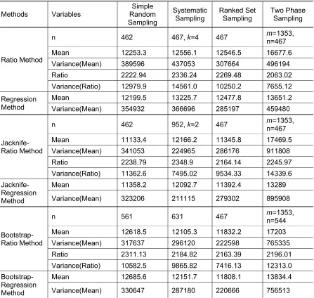
Results of various designs are shown in table1 below:

Table 1: Results of Various Designs

Methods Variables Random Simple Sampling

Systematic Sampling

Ranked Set Sampling

Two Phase Sampling

Ratio Method

n 462 467, k=4 467 m=_n=467 1353,

Mean 12253.3 12556.1 12546.5 16677.6

Variance(Mean) 389596 437053 307664 496194

Ratio 2222.94 2336.24 2269.48 2063.02

Variance(Ratio) 12979.9 14561.0 10250.2 7655.12 Regression

Method

Mean 12199.5 13225.7 12477.8 13651.2

Variance(Mean) 354932 366696 285197 459480

Jacknife-Ratio Method

n 462 952, k=2 467 m=_n=467 1353,

Mean 11133.4 12166.2 11345.8 17469.5

Variance(Mean) 341053 224965 286176 911808

Ratio 2238.79 2348.9 2164.14 2245.97

Variance(Ratio) 11362.6 7495.02 9534.33 14339.6

Jacknife-Regression Method

Mean 11358.2 12092.7 11392.4 13289

Variance(Mean) 323206 211115 279302 895908

Bootstrap-Ratio Method

n 561 631 467 m=_n=544 1353,

Mean 12618.5 12105.3 11832.2 17203

Variance(Mean) 317637 296120 222598 765335

Ratio 2311.13 2184.82 2163.39 2196.01

Variance(Ratio) 10582.5 9865.82 7416.13 12313.0

Bootstrap-Regression Method

Mean 12685.6 12151.7 11808.1 13834.4

Variance(Mean) 330647 287180 220666 756513

Table 2: Multistage with PPS and Systematic

n 380 Mean 12069.9 Variance(Mean) 518976

4. Conclusion

From the above results, we conclude that Ranked set sampling with ratio and regression methods, is the most efficient among other designs for HIES data. Jacknife and Bootstrap also performed fairly well with Ranked set sampling.

Bibliography

1. Chaudhuri, A. and Stenger, H. (1992). Survey Sampling Theory and

Methods. Marcel Dekker, Inc.

2. Cochran, W. G. (1977). Sampling Techniques. (3rd Ed.). John Wiley and

Sons, New York.

3. Government of Pakistan. HIES Data of 1998-99 and 2001-02 by Statistical Division, Federal Bureau of Statistics, Islamabad.

4. Kish, L. (1965). Survey Sampling. John Wiley & Sons, New York.

5. Lohr (1999). Sampling Design and Analysis. Brooks/Cole Publishing Co.

6. Mukhopadhyay, P. (1998). Theory and Methods of Survey Sampling.

Prentice-Hall of India, New Delhi.

7. Shao, J. and Tu, D. (1995). The Jacknife and Bootstrap. Springer-Verlag

New York, Inc.

8. Som R.K. (1973). A Manual of Sampling Techniques. Heinemann

Educational Books, London.

9. Sukhatme, P.V. and Sukhatme, B.V. (1984). Sampling Theory of Survey

with Applications. Iowa State University Press, USA.