Problems Arising from Rigid Body Dynamics
Iman Mohamad Sharaf
Higher Technological Institute, Egypt [email protected]
Abstract
An active set algorithm is introduced for positive definite and positive semi definite linear complementarity problems. The proposed algorithm is composed of two phases. Phase 1, the feasibility phase and phase 2, the optimality phase. In phase 1, the ellipsoid method is employed to test for feasibility and provide an advanced starting point if the problem is feasible. Providing such a warm start permits a good estimate of the active set. In phase 2, a criterion based on the complementarity condition is used to detect the working set per iteration until optimality is reached. This criterion leads to a valuable reduction in the size of the problem solved per iteration to obtain a search direction. Numerical examples are solved to illustrate the performance of the algorithm and a practical example in rigid body dynamics is solved to demonstrate the usage of the algorithm to solve such problems.
Keywords: Mathematical programming; Linear complementarity problems; Convex quadratic programming; Active set methods; Rigid body dynamics.
1. Introduction
The linear complementarity problem (LCP) is one of the widely studied problems in optimization. The LCP first emerged as the Karush-Kuhen-Tucker (KKT) optimality conditions for linear programming (LP) and quadratic programming (QP); it has often been described as a fundamental problem Billups and Murty (2000). Besides covering several important classes of mathematical programming problems such as LP, convex quadratic programming (CQP), Nash equilibrium points for nonzero sum games, several economic equilibrium problems and the knapsack problem, the LCP is also used to model many applications such as the contact problem, the obstacle problem, the porous flow problem, the journal bearing problem and many other free boundary problems Wang (2010).
For a given real vector and a given real matrix M the LCP (q, M) finds the vector which satisfy the constraints
,
or show that no such vector exists, where “T” denotes the matrix transpose. A LCP is said to be feasible if the feasible set
{ }
and is said to be solvable if the solution set
Alternatively, the LCP finds the pair of vectors by setting in the previous constraints.
There is a close connection between the LCP and the QP
(1)
The feasible set of (1) is exactly . To compensate for the fact that the matrix M may be asymmetric, it is customary to use the following equivalent representation of the objective function
Any solution of the LCP is an optimal solution of (1). However the converse is not valid unless the optimal objective function value of (1) is zero (Cottle et al. 1989).
The class of the matrix M has always played a prominent role in the LCP theory since much depends on knowing the matrix through which the particular LCP is defined. The key properties of feasibility, solvability, uniqueness, convexity and the applicability of a certain method are related to the matrix class. For example, the LCP has a unique solution if and only if M belongs to the class P of matrices with positive principal minors, a LCP with a positive semi definite matrix has a nonempty convex polyhedral solution set Cottle et al. (1989). As the LCP belongs to the class of NP-complete problems; therefore it is not expected to find an efficient solution method for the problem without a special property of the matrix M Illes and Nagy (2007). In general, some algorithms relay on a certain matrix class, other algorithms perform well under a broad range of matrix classes Kostreva and Yang (2004). Nowadays, there are more than 50 matrix classes discussed in the LCP literature Cottle (2010).
Several methods have been developed to solve the LCP. Pivotal methods are the early methods for solving the LCP. These methods utilize different pivot rules. Despite their efficiency in solving small problems, they do not exploit sparsity effectively and are unsuitable for large applications Morales et al. (2007). The most salient pivoting algorithms are Lemke’s algorithm and the principal pivoting algorithm introduced by Cottle and Dantzig Rüst (2007). Interior point methods have been inspired by the algorithms that have been used for solving linear programs in polynomial time developed originally by Karmarker. These methods produce a sequence of points that follow the so-called central path, a nonlinear path from a strictly feasible point towards the solution. They are effective for solving large and ill-conditioned LCPs; their main drawbacks are the high cost per iteration and that they may not yield a good estimate of the solution when terminated early Morales et al. (2007). Several algorithms have been proposed to lessen the required computations per step Lešaja et al. (2012), Zangiabadi and Mansouri (2012). Yet, interior point algorithms remain computationally more expensive than active set algorithms Ferreau et al. (2014).
Edalapanah (2013), Popa et al. (2015), Zhang (2015). They also have a low computational cost per iteration and have been shown to be convergent under certain conditions Morales et al. (2007). Yet, they can be very slow for medium to large scale and ill-conditioned problems Archavaleta et al. (2009). The last class of methods is the conventional algorithms for solving QPs such as the gradient projection methods and the active set methods. Extensive coverage of LCP theory is available in Cottle, Pang and Stone (1992) and Murty (1988).
The goal of active-set methods is to predict the active set, the set of constraints that are satisfied with equality, at the solution of the problem. A working set is chosen and is then updated in each step until optimality is reached. The search directions are taken as the solution of a KKT-system formed from the QP Hessian and the working-set constraint gradients. The conventional active-set methods are divided into two phases; the feasibility phase and the optimality phase. An advantage of active-set methods is that they are well-suited for warm starts.
In this article an active set algorithm is proposed that uses different approaches than that used by the conventional active set algorithms in both phases. In phase 1, the ellipsoid method is employed to test for the problem feasibility and to provide a warm-start if the problem is feasible Hassan et al. (2007). In phase 2, a criterion based on the complementarity condition is used to detect the working set per iteration until optimality is reached. This criterion leads to a reduction in the size of the linear system solved each step to get a search direction.
The article is organized as follows. Section 2 presents the properties of PD and PSD matrices. A brief account on active set methods and the ellipsoid method is given in sections 3 and 4. The proposed algorithm is introduced in section 5. In section 6 a numerical example and a practical example are solved. Finally, the conclusion is given in section 7.
2. PD and PSD matrices and the LCP
The mathematical structure of the LCP has inspired several researchers to study the matrix properties and its implication regarding the existence and uniqueness of solution and the formulation of a suitable method of solution (Li et al. 2010). In fact, much of the LCP theory and algorithms are based on the assumption that the matrix belongs to a particular class of matrices (Das 2005). The class of PD and PSD matrices arises in numerous applications in Mathematical Programming, Statistics, Complementarity Modeling, Engineering and Management Sciences Neogy and Das (2013), Bhimashankaram et al. (2013).
The feasible set and the complementarity ellipsoid intersects in only one point that lies on the boundary which is the unique solution of the problem Murty, (1988).
While a matrix is said to be positive semi definite if the quadratic form is nonnegative for every nonzero vector . For a PSDLCP the feasible set may be empty. Else, if , the solution set is a convex polyhedral and the LCP in this case may have a unique solution or it may have multiple solutions Chen and Xiang (2014). These solutions lie in the convex set Murty (1988).
3. Active-set methods
A variety of methods have been proposed to solve QP. Two major successful approaches are active-set methods and interior point methods. These methods have proven to be quite effective at solving problems with thousands of variables and constraints Byrd et al.
(2004). While active set methods need on average substantially more iterations than interior point methods, an active set iteration is computationally much cheaper Ferreau et al. (2014). In addition, active set methods are more robust and better suited for warm starts (where a good estimate of the optimal active set is used to start the algorithm); therefore there is a renewed interest in new active-set approaches (Leyffer 2005).
Active-set methods originated as extensions of the simplex method for solving LPs. The basic idea of active-set methods is to fix a working set, a maximal linearly independent subset of the active constraints, and to solve the resulting constrained QP problem. The working set is then updated in each step until optimality is reached. The search directions are taken as the solution of a KKT-system formed from the QP Hessian and the working-set constraint gradients. There are two main approaches used, the binding-direction methods and the nonbinding- direction methods. In the binding-direction methods, every direction lies in the null space of the working set matrix, so that all working-set constraints are active, while in the nonbinding-direction methods directions are inactive with respect to one of the constraints in the working set (Wong 2011).
Active set methods can be divided into primal, dual and parametric (Ferreau et al. 2014). When finding a feasible starting point primal active-set methods generate a sequence of primal feasible iterates until dual feasibility is achieved, hence an optimal solution is obtained. Dual active-set methods for CQP generate a sequence of dual feasible iterate until primal feasibility is achieved, hence an optimal solution is obtained. In primal active set methods if no feasible starting point is known an identification phase, named phase one, is used to generate a feasible point or detect infeasibility, while dual active-set methods do not require the usage of phase one. One relatively recent approach to solve QP problems are parametric active-set methods that are based on tracing the solution among the solution along a linear homotopy between a QP problem with known solution and the QP problem to be solved (Ferreau et al. 2014).
program (EQP) approach in which the active set identification and optimization computations are performed in two separate phases. In the identification phase a linear program is solved to estimate the active set. In the second phase, an EQP is solved involving only the constraints that are active at the solution of the linear program. In contrast, SQP methods follow a so-called inequality constrained quadratic program (IQP) approach in which the new iterate and the new estimate of the active set are computed simultaneously by solving an inequality sub problem (Hei et al. 2008).
4. The ellipsoid method
The ellipsoid method was first introduced by Yudin and Nemirovskii (1976), then clarified by Shor (1977); they were interested in applying the method to convex, not necessarily differentiable, optimization. Later Khachiyan (1979) modified the method to derive the first polynomial time algorithm for LP. Although the algorithm is better theoretically than the Simplex method, which is an exponential time algorithm, practically it is slower and not competitive with the Simplex method (Bland et al. 1981). Yet, it remains as an important theoretical tool to develop polynomial time algorithms for a large class of convex optimization problems (Beck and Sabach 2012)
The ellipsoid method is designed to solve decision problems rather than optimization problems (Rebennack 2008). Therefore the decision problem of finding a feasible point to the system of linear inequalities ,where and , is solved in an innovative way. The goal is to find the vector satisfying the system of linear inequalities or to prove that such vector does not exist.
The algorithm starts with an initial ellipsoid containing the solution set of . The center of the ellipsoid is a candidate for a feasible point of the problem in each step. After checking whether this point satisfies all the linear inequalities, either the point is feasible and the algorithm terminates, or this point violates one or more of the given inequalities. One of the violated constraints is used to construct a new ellipsoid of smaller volume having a different center. The procedure is repeated until either a feasible point is attained or maximum number of iterations is reached which implies that the system is infeasible.
5. The proposed algorithm
The algorithm is a two phase iterative method that provides an estimate of the active set at the solution. In the first phase (the feasibility phase) the ellipsoid method is employed to compute an initial point for phase 2 or detect infeasibility. In the second phase (the optimality phase) a criterion based on the complementarity condition is used to define the working set until optimality is reached.
5.1. Phase 1
An n- dimensional ellipsoid with center is formulated algebraically as the set
{ }
with symmetric, positive definite, real valued matrix B. The initial ellipsoid
For each iteration , it is checked whether the current ellipsoid center satisfies the linear inequality system , where [ ] and [ ] . If all the inequalities are satisfied, is a feasible point set and the algorithm terminates. Otherwise, there is at least an inequality which is violated by . One of the violated constraints is used to cut the ellipsoid into two parts. A new ellipsoid , which is smaller in volume than is generated to enclose the part that contains the optimal solution. The updating formulas are as follows (Bland et al. 1981):
√( ) (2)
( ( ( )( )) ) (3)
where are the step, dilation and expansion parameters.
Several simple modifications to these parameters were introduced to improve the convergence of the algorithm. One of these modifications is to use the deepest cut to generate smaller ellipsoids in which the parameters are given by
√
By computing for each violated inequality the deepest possible cut is chosen; i.e. the cut corresponding to the largest , where . If the parameter in the step satisfies , then and the problem is infeasible.
Clearly, if the number of iterations exceeds an upper limit given by
where L is the length of the binary encoding of data,
⌈ ∑( (| | )) ∑ | |
⌉
this also indicates that is empty and the problem is infeasible.
Having obtained a feasible interior point, a feasible boundary point can be obtained by taking a step in the direction of the steepest descent .
Therefore, the initial point is given by , where is the step size. It is required to take the maximum step in the direction such that the ith constraint is active and none of the other constraints is violated. The step length taken is computed as:
To avoid the constraints violation, the step length must be taken as:
This ends phase 1 and the boundary point is taken as an initial point for phase 2.
5.2. Phase 2
This is the optimality phase in which complementarity is satisfied, the complementarity function , while feasibility is maintained. The value of is calculated at the point . If , a pre-specified convergence tolerance, then this point is the solution of the problem and the algorithm terminates. Else, phase 2 of the algorithm proceeds as follows.
Since the complementarity condition requires that either the variable
or the ith constraint is active, i.e. , some of the constraints will be assumed to be active. The constraint function whose value at a current boundary point is less than a certain value , which will be referred to as the threshold value , will be considered active. While the constraint function whose value is more than this value will be considered inactive. Accordingly, for the constraints satisfying
the corresponding is set equal to zero. Meanwhile, any is kept
fixed. The threshold value will be taken as ⁄ where is the reduction factor. Throughout the article this factor is initially set to zero. If the working set is empty, it is incremented by one until at least one constraint lies in the working set.
After choosing the working set a reduced system of linear equations, which will be denoted as , is solved to obtain the nonzero variables. This reduced system is obtained from the system of linear equations after omitting the inactive constraints from the system and the columns corresponding to the zero variables from the matrix . This leads to a valuable reduction in the size of the problem solved in contrast to most of the active set methods that solves in each step a Karush-Kuhn-Tuker (KKT) system formed from the QP Hessian and the working – set constraint gradients (Wong 2011). The solution of the system together with the zero variables gives a complementary solution . If the point is feasible, then this point is a solution of the problem. Else, a step is taken from in the direction , which is a descent direction since
and , without violating any of the constraints to get a new boundary point with , where
The previous steps are repeated until a point is attained with , or no further improvements could be made.
solution under the hypothesis of existence of minimizers (Rao, 2009). In the proposed algorithm, the used direction is a usable feasible direction, i.e. one that reduces the objective function without violating the feasibility conditions, since the step taken in this direction violates no constraint and reduces the complementarity function.
The algorithm can be summarized as follows
The algorithm
Input n = number of variables.
= starting ellipsoid, the matrix and the vector . Set , .
Output A point or detect that .
Step 1. Finding a feasible point. Check whether .
If , set , go to step 2.
Else if , compute for the violated constraints by . If , return , terminate.
Else, select the constraint with the largest ,calculate . Update the ellipsoid using formulas (2) and (3).
, if , return , terminate. Else, repeat step 1.
Step 2. Finding an initial boundary point.
Find , where
Step 3. Choosing the working set. Calculate
If , terminate. Else, Set .
While the working set =
Compute ⁄
If for all i, .
Else, the constraints satisfying are added to the working set. For , set .
End.
Step 4. Solve the reduced system for .
If then , terminate. Else, compute
Find , where
6. Examples
6.1. Numerical Examples
Example 1
Consider the LCP
(
) (
).
A starting ellipsoid is used. Applying the proposed algorithm, Phase 1 gives a starting boundary point in 2 iterations. The complementarity function at this point and ⁄ .
The value of the constraints function is the first constraint is assumed to be active, while and . Solving the reduced system , where gives . Thus phase 2 gives the exact solution in 1 iteration. When applying Lemke’s algorithm to solve this problem (Murty 1988), the solution is achieved after 8 iterations. In fact, the primary computational step in phase 2 is the same as that of Lemke’s algorithm (the elementary row operation). Yet, the number of variables used by phase 2 of the proposed algorithm is less than the variables used by Lemke’s algorithm by more than half.
Example 2
Consider the LCP
(
)
(
)
.
A starting point is found in one iteration. The complementarity function at this point , accordingly
⁄ . Computing the values of the constraints function . Then the leading three constraints are assumed to be active while is assumed to be zeros. Solving the reduced
system with (
) (
) gives
(
)
Since is
infeasible, the descent direction is computed, and
assumed to be zeros. Solving the reduced system with ( ) ( ) gives
which is the solution.
6.2. A practical example
Computing the reaction forces arising between rigid bodies in contact is useful in a wide variety of applications including robotics, computer graphics, animation, haptics and mechanical simulation (Lloyd 2005). The typical model of contacting rigid bodies is composed of the Newton-Euler dynamics equations, non-penetration constraints, unilateral-force constraints and frictional constraints. Choosing the suitable coordinates, the equations and constraints rigid body contacts can be formulated as a linear complementarity problem (Chakraborty et al. 2014, Elkahoui et al. 2001, Yamane and Nakamura 2008).
A common problem in rigid body physics engines is jitter, which affect piles of objects in particular. Bodies close to rest can visibly jitter, it is required to avoid jitter. Piles require stable simulation of static friction, dynamic friction and resting contact (Tonge et al. 2012). The following LCP model of jitter free stacking is according to Kenwright and Morgan (2012), and Tonge, Benevolenski, and Voroshilov (2012).
Consider a scene having rigid bodies with positions , external forces , forces applied at the contact points and masses . Collision detection identifies contacts between the rigid bodies, represented by the constraints with Jacobian ⁄ . Constraints stabilization and friction are omitted for simplicity of modeling. Contacts must satisfy the velocity Signorini condition: forces must not be attractive ( velocities must move the system out of penetration ( , and a force should be applied at a contact only if the contact is not separating ( . The resulting continuous model is the following differential variational inequality:
̈ ̇
The model is discretized using a semi-implicit stepping scheme with time step h, and introduce the constraint impulse .
Multiplying both sides by yields
(
This discretized model is a LCP rather than a linear system due to the Signorini condition. The matrix and the vector of the LCP (q, M) are given by:
and
complementary feasible solution to this LCP is a pair of vectors , where the vector is the vector of relative accelerations at the contact points and the vector is the vector of forces applied at the contact points.
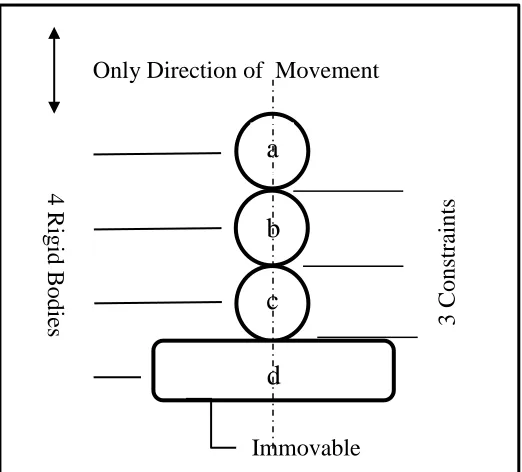
Consider the example given by Kenwright and Morgan (2012). The configuration consists of three objects equal in mass (one unit each) stacked upon one another on an immovable surface. When an external force is applied downward due to gravity, it is required to calculate the modified force to stop the objects from moving downwards. The configuration is shown in Figure 1.
Figure 1. Numerical Example (Kenwright and Morgan 2012)
The mass matrix and Jacobian are as follows:
( )
(
) (
),
where the number of columns represents the number of rigid bodies (4) and the number of rows represent the number of constraints (3 contact positions).
The velocity and external force vectors are as follows:
( ) (
),
4
R
ig
id
B
odies
3 Con
stra
int
s
Immovable
a
b
d
c
all the objects have zero initial velocities, except the second to top one which is set to have an internal downward velocity.
Thus the matrix (
) and the vector (
)
The proposed algorithm is used to solve the problem. A boundary point is obtained in one step, then the solution after two steps solving a reduced system with
in each step. This value is then put back into the system to get the constraint
force required to prevent the movement of the objects downwards
.
7. Conclusion
In this article an active set algorithm is proposed. It solves the LCP for the vector z only in contrast to most of the LCP algorithms, e.g. pivoting algorithms and interior point algorithms, which solve the problem for the pair of vectors (w, z) thus reducing the number of variables. In addition pivoting algorithms as Lemke’s algorithm is numerically sensitive, especially in the presence of redundant contacts, and requires working with large matrices; e.g. the LCP matrix for a problem with 16 contacts and an 8 sided friction cone approximation has a size of 160 (Lloyd 2005); interior point algorithms are computationally more expensive than active set algorithms (Ferreau et al. 2014).
The algorithm is composed of two phases. In phase 1, the ellipsoid method is employed to test for the problem feasibility and to provide a starting point for phase 2 in case of feasibility. This starting point is an advanced point, this warm start allows a good estimate of the active set, accordingly the iterations required to reach optimality is reduced. In phase 2, a criterion based on the complementarity condition is used to detect the working set per iteration until optimality is reached. This criterion leads to a reduction in the size of the linear system solved each step to get a search direction. Numerical examples were solved to test the algorithm. A simple practical example was given to illustrate the applicability of the algorithm to solve such problems.
References
1. Adler, I., R.W. Cottle and S. Verma (2009). New characterization of row sufficient matrices. Linear Algebra and its Applications, 430, 2950-2960.
2. Arechavaleta, G., E. Lopez-Damian and J. Morales (2009). On the use of iterative solvers for dry frictional contacts in grasping. Advanced Robotics, ICAR 2009. 3. Beck, A., S. Sabach (2012). “An improved ellipsoid methos for solving convex
differentiable optimization problems.” Operations Research Letters, 40: 541-545. 4. Bhimashankaram, P., T. Parthasarathy, A. L. N. Murthy, and G. S. R. Murthy
(2013). “Complementarity Problems and Positive Definite Matrices.” Algorithmic operations Research 7: 94-102.
6. Bland, G. B., D. Goldfarb, M. J. Todd (1981). The Ellipsoid Method: A survey. Operations Research, 28(6), 1039-1091.
7. Byrd, H. B., N. I. M. Gould, J. Nocedal, R. A. Waltz (2004). An Active-Set
Algorithm for Nonlinear Programming and Equality Constrained
Subproblems.mthematical programming ser B. 100, 27-48.
8. Chakraborty N., S. Berard, S. Akella, J. Trinkle (2014). A geometrically implicit time-stepping method for multibody systems with intermittent contact. International Journal of Robotics Research, 33(3), 426-445.
9. Chen, X. and S. Xiang (2014). Sparse Solutions of Linear Complementarity Problems. www.polyu.edu.hk
10. Cottle, R. W. (2010). A field guide to the matrix classes found in the literature of the linear complementarity problem. Journal of Global Optimization, 46(4), 571-580.
11. Cottle, R. W., J. Pang, and R. Stone (1992). The Linear Complementarity Problem. New York: Academic Press.
12. Cottle, R. W., J. S. Pang and V. Venkateswaran (1989). Sufficient Matrices and the Linear Complementarity problem. Linear Algebra and its applications, 114/115,231-249.
13. Das, A. K. (2005). Properties of some Matrix Classes in Linear complementarity Problem. D.Sc. Thesis, Indian Statistical Institute, Kolkata, India.
14. El Kahoui, M., A. Weber and B. Eberhardt, (2001). Improved algorithms for linear complementarity problems arising from collision response. Mathematics and computers in simulation, 56(1), 69-93.
15. Ferreau, H. J., C. Kirches, A. Potschka, H. G. Bock and M. Diehel, (2014). qpOASES: a parametric active-set algorithm for quadratic programming. Mathematical Programming Computaion, 6, 327-363.
16. Hassan, A. S. O., Abdel-Malek, H. L. & Sharaf, I. M. (2007). An exterior point algorithm for some linear complemetarity problems with applications.
Engineering Optimization, 39 (6), 661-677.
17. Hei, L., J. Nocedal, R. A. Waltz (2008). A Numerical Study of Active-Set and Interior-point Methods for Bound Constrained Optimization. Modelind, Simulation and Optimization, 273-292.
18. Illes T. and M. Nagy (2007). “A Mizuno-Todd-Ye predictor-corrector algorithm for sufficirnt linear complementarity problems.” European Journal of Operational Research 181: 1097-1111.
19. Kenwright, B., G. Morgan (2012). Practical introduction to Rigid Body Linear Complementarity problem Constraint Solvers. Algorithmic and Architectural Gaming Design: Implementation and Development. Chapter 8, pp.159-202. DOI:10.4018/978-1-4666-1634-9.ch008
20. Kostreva, M. M. and X. Q. Yang (2004). Unified approach for solvable and unsolvable linear complementarity problems. European Journal of Operational Research, 158, 409-417.
22. Leyffer, S. (2005). The Return of Active Set Method. Mathematics and Computer science Division, Preprint ANL/MCS-P1277-0805.
23. Li, Zukui and G. I. Marianthi (2010). A method for solving the general parametric linear complementarity problem. Annals of operations Research, 181(1), 485-501. 24. Lloyd, J. E. (2005). Fast Implementation of Lemke’s Algorithm for Rigid Body Contact Simulation. Robotics and Automation, Proceedings of the 2005 IEEE International Conference, 4538-4543.
25. Loomis A., D. Balkcom (2006). “Computation reuse of rigid-body dynamics.” Proceedings of the 2006 IEEE/RSJ. International Conference on Intelligent robots and Systems, Bejing, China, October 9-15.
26. Morales, J. L., J. Nocedal, and M. Smelyanskiy (2008). An Algorithm for the Fast solution of Symmetric Linear Complementarity Problems. Numerishe Mathematik 111(2): 251-268.
27. Murty, K. G. (1988). Linear complementarity, linear and nonlinear programming. In Sigma Series in Applied Mathematics. Berlin: Heldermann.
28. Najafi, H. S., Edalatpanah, S. A. (2013). SOR-Like Methods for Non-Hermitian Positive Definite Linear Complementarity Problems. Advanced Modeling and optimization, 15, 3, 697-704.
29. Neogy, S. K. and A. K. Das (2013). On weak generalized positive subdefinite matrices and the linear complementarity problem. Linear and Multilinear Algebra, 61(7), 945-953.
30. Popa C., T. Preclik, U. Rude (2015). Regularized solution of LCP problems with application to rigid body dynamics. . Numerical Algorithms (69), 145-156. 31. Rao, S. S. (2009). Engineering Optimization: Theory and Practice. Fourth
Edition. Hoboken, New Jersy: John Wiley & Sons.
32. Rebennack, S., (2008). Ellipsoid Method. Encyclopedia of Optimization, Second Edition, Springer, 890-899.
33. Rüst, L.Y. (2007). The P-Matrix Linear Complementarity Problem: generalizations and Specializations. D.Sc. diss., Swiss Federal Institute of Technology, Zurich.
34. Tonge, R., F. Benevolenski, A. Voroshilov (2012). “Mass Splitting for Jitter-free Parallel Rigid Body Simulation”. ACM TOG 31(4): article No. 105.
35. Yamane, K., and Y. Nakamura, (2008). “A Numerically Robust LCP solver for Simulating Articulated Rigid Bodies in Contact”. In Proceedings of Robotics: Science and Systems IV, Zurich, Switzerland.
36. Wang, X. (2010). “Properties of Classes of Linear Transformations in the semidefinite linear complementarity problem.” Ph.D. diss., UC Berkley.
37. Wong, E. (2011). Active-set methods for Quadratic Programming. Ph.D. diss., University of California, San Diego.
38. Zangiabadi, M. and H. Mansouri, (2012). Improved infeasible interior point algorithm for linear complementarity problems. Bulletin of the Iranian Society, 38(3), 787-803.