R E S E A R C H
Open Access
A normalization strategy for comparing tag count
data
Koji Kadota
1,2*, Tomoaki Nishiyama
3and Kentaro Shimizu
1Abstract
Background:High-throughput sequencing, such as ribonucleic acid sequencing (RNA-seq) and chromatin immunoprecipitation sequencing (ChIP-seq) analyses, enables various features of organisms to be compared through tag counts. Recent studies have demonstrated that the normalization step for RNA-seq data is critical for a more accurate subsequent analysis of differential gene expression. Development of a more robust normalization method is desirable for identifying the true difference in tag count data.
Results:We describe a strategy for normalizing tag count data, focusing on RNA-seq. The key concept is to remove data assigned as potential differentially expressed genes (DEGs) before calculating the normalization factor. Several R packages for identifying DEGs are currently available, and each package uses its own normalization method and gene ranking algorithm. We compared a total of eight package combinations: four R packages (edgeR, DESeq,baySeq, andNBPSeq) with their default normalization settings and with our normalization strategy. Many synthetic datasets under various scenarios were evaluated on the basis of the area under the curve (AUC) as a measure for both sensitivity and specificity. We found that packages using our strategy in the data normalization step overall performed well. This result was also observed for a real experimental dataset.
Conclusion:Our results showed that the elimination of potential DEGs is essential for more accurate normalization of RNA-seq data. The concept of this normalization strategy can widely be applied to other types of tag count data and to microarray data.
Background
Development of next-generation sequencing technolo-gies has enabled biological features such as gene expres-sion and histone modification to be quantified as tag count data by ribonucleic acid sequencing (RNA-seq) and chromatin immunoprecipitation sequencing (ChIP-seq) analyses [1,2]. Different from hybridization-based microarray technologies [3,4], sequencing-based technol-ogies do not require prior information about the gen-ome or transcriptgen-ome sequences of the samples of interest [5]. Therefore, researchers can profile the expression of not only well-annotated model organisms but also poorly annotated non-model organisms. RNA-seq in such organisms enables the gene structures and expression levels to be determined.
One important task for RNA-seq is to identify differ-ential expression (DE) for genes or transcripts. Similar to microarray analysis, we typically start the analysis with a so-called “gene expression matrix,” where each row indicates the gene (or transcript), each column indi-cates the sample (or library), and each cell indiindi-cates the number of reads mapped to the gene in the sample. In general, there are two major factors for accurately quan-tifying and normalizing RNA-seq data: gene length and sequencing depth (or total read counts). Normalization by gene length is important for comparing different genes within a sample because longer genes tend to have more reads to be sequenced [6]. Previous approaches for normalizing length include defining an effective length of a gene that may have two or more transcript isoforms of different lengths, and normalizing by the length [7-11].
Normalization by sequencing depth is particularly important for comparing genes in different samples because different samples generally have different total * Correspondence: [email protected]
1Agricultural Bioinformatics Research Unit, Graduate School of Agricultural
and Life Sciences, The University of Tokyo, 1-1-1 Yayoi, Bunkyo-ku, Tokyo 113-8657, Japan
Full list of author information is available at the end of the article
read counts. Previous approaches include (i) global scal-ing so that a summary statistic such as the mean or upper-quartile value of read counts for each sample (or library) becomes a common value and (ii) standardiza-tion of distribustandardiza-tion so that the read count distribustandardiza-tions become the same across samples [12-15]. Some groups recently reported that over-representation of genes with higher expression in one of the samples, i.e., biased dif-ferential expression, has a negative impact on data nor-malization and consequently can lead to biased estimates of true differentially expressed genes (DEGs) [15,16]. To reduce the effect of such genes on the data normalization step, Robinson and Oshlack reported a simple but effective global scaling method, the trimmed mean of M values (TMM) method, where a scaling fac-tor for the normalization is calculated as a weighted trimmed mean of the log ratios between two classes of samples (i.e., Samples A vs. B) [16]. The concept of the TMM method is the basis for developing our normaliza-tion strategy.
In this paper, we focus on normalization related to sequencing depth as well as the TMM normalization method. We believe the TMM method can be improved. Consider, for example, a hypothetical dataset containing a total of 1000 genes, where (i) 200 genes (i.e., 200/1000 = 20%) are detected as DEGs when comparing Samples A vs. B (PDEG = 20%), (ii) 180 of the 200 DEGs are
highly expressed in Sample A (i.e., PA = 180/200 =
90%), (iii) the dataset can be perfectly normalized by applying a normalization factor calculated based only on the remaining 800 non-DEGs, and (iv) individual DEGs (or non-DEGs) have a negative (or positive) impact on calculation of the normalization factor. In this case, the two parameters should ideally be estimated as PDEG=
20% andPA= 90%. Currently, the TMM method
impli-citly uses fixed values for these two parameters (i.e., PDEG= 60 andPA= 50) unless users explicitly provide
arbitrary values [16,17]. This is probably because an automatic estimation of the PDEG value is practically
difficult.
Hardcastle and Kelly [18] recently proposed an R [19] package,baySeq, for differential expression analysis of RNA-seq data. A notable advantage of this method is that an objective PDEGvalue is produced by calculating
multiple models of differential expression. This method also inspired us in our improvement of the normaliza-tion of RNA-seq data. Our normalizanormaliza-tion strategy, named TbT, consists of TMM [16] and baySeq [18], used twice and once respectively in a TMM-baySeq -TMM pipeline. We show the importance of estimating the PDEG value according to the true PDEG value for
individual datasets. The results were obtained using simulated and real datasets.
Results and Discussion
RNA-seq data must be normalized before differential expression analysis can be conducted on them. Some R packages exist for comparing two groups of samples [17,18,20,21], and each package uses its own normaliza-tion method and gene ranking algorithm. For example, the R package edgeR [17] uses the TMM method [16] for data normalization and an exact test for negative binomial (NB) distribution [22] for gene ranking. A good normalization method coupled with gene ranking methods should produce good ranked gene lists where true DEGs can easily be detected as top-ranked and non-DEGs are bottom-ranked, when all genes are ranked according to the degree of DE.
Following from our previous study [23-25], the area under the receiver operating characteristic (ROC) curve (i.e., AUC) values were used for evaluating individual combinations based on sensitivity and specificity simul-taneously. A good combination should therefore have a high AUC value (i.e., high sensitivity and specificity). In the remainder of this paper, we first describe our nor-malization strategy (called TbT). We then evaluate a total of eight package combinations: four R packages for differential expression analysis (edgeR[17],DESeq [20], baySeq [18], andNBPSeq[21]) with default normaliza-tion settings (which we call edgeR/default, DESeq/ default, baySeq/default, and NBPSeq/default) and the same four packages with TbT normalization (i.e.,edgeR coupled with TbT (edgeR/TbT),DESeq/TbT, baySeq/ TbT, andNBPSeq/TbT). Finally, we discuss guidelines for meaningful differential expression analysis.
Note that the execution of the baySeqpackage was performed using data after scaling for the reads per mil-lion (RPM) mapped reads in each sample. The proce-dure in the baySeq package and in the other three packages (edgeR, DESeq, and NBPSeq) is not intended for use with RPM-normalized data, i.e., the original raw count data should be used as the input. However, we found that the use of RPM-normalized data generally yields higher AUC values compared to the use of raw count data when executing the baySeqpackage. We also found that the use of RPM data did not positively affect the results when the other three packages were exe-cuted. Accordingly, all of the results relating to the bay-Seq package were obtained using the RPM-normalized data. This includes step 2 in the TbT normalization and the gene ranking of DEGs using two baySeq-related combinations (baySeq/TbT andbaySeq/default).
Outline of TbT normalization strategy
simulation data that are negative binomially distributed (three libraries from Sample A vs. three libraries from Sample B; i.e., {A1, A2, A3} vs. {B1, B2, B3}). The
simula-tion condisimula-tions were that (i) 20% of genes were DEGs (PDEG= 20%), (ii) 90% ofPDEGwas higher in Sample A
(PA= 90%), and (iii) the level of DE was four-fold.
The NB model is generally applicable when the tag count data are based on biological replicates. It has been noted that the variance of biological replicate read counts for a gene (V) is higher than the mean (μ) of the read counts (e.g., V =μ + jμ2 where j> 0) and that the extra dispersion parameterjtends to have large (or small) values when μ is small (or large) [20,21]. To mimic this mean-dispersion relationship in the simula-tion, we used an empirical distribution of these values (μandj) calculated from Arabidopsis data available in theNBPSeqpackage [21]. For details, see the Methods section.
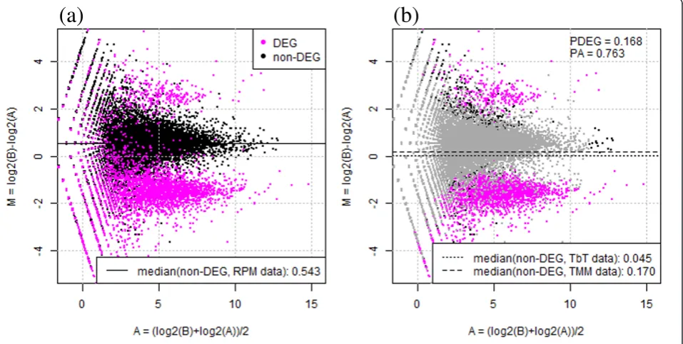
An M-A plot of the simulation data, after scaling for RPM reads in each library, is shown in Figure 1a. The horizontal axis indicates the average expression level of a gene across two groups, and the vertical axis indicates log-ratios (Sample B relative to Sample A). As shown by the black horizontal line, the median log-ratio for non-DEGs based on the RPM-normalized data (0.543) has a clear offset from zero due to the introduced DEGs with
the above three conditions. Therefore, the primary aim of our method is to accurately estimate the percentage of true DEGs (PDEG) and trim the corresponding DEGs
so that the median log-ratio for non-DEGs is as close to zero as possible when our TbT normalization factors are used.
To accomplish this, our normalization method con-sists of three steps: (1) temporary normalization, (2) identification of DEGs, and (3) final normalization of data after eliminating those DEGs. We used the TMM method [16] at steps 1 and 3 and an empirical Bayesian method implemented in thebaySeq package [18] at step 2. Other methods could have been used, but our choices seemed to produce good ranked gene lists with high sensitivity and specificity (i.e., a high AUC value). We observed that the median log-ratio for non-DEGs based on our TbT normalization factors (0.045) was closer to zero than the log-ratio based on the TMM normaliza-tion factors (0.170) that corresponds to the result of TbT right after step 1 (Figure 1b).
This result suggests the validity of our strategy of removing potential DEGs before calculating the normali-zation factor. Recall that the true values forPDEG and
PAin this simulation were 20% and 90%, respectively.
Our TbT method estimated 16.8% ofPDEGand 76.3% of
PA. We found that 64.4% of the estimated DEGs were
(a)
(b)
Figure 1Outline of TbT normalization strategy. Left panel: M-A plot for negative binomially distributed simulation data from Ref. [21], after scaling for RPM mapped reads in each sample. Magenta and black dots indicate DEGs (20% of all genes;PDEG= 20%) and non-DEGs (80%),
respectively. 90% of all DEGs is four-fold higher in Sample A than B (PA= 90%). Each dot represents a gene. Right panel: same plot but colored
differently. TbT estimates 16.8% ofPDEGusing this data. Gray dots indicate genes estimated as non-DEGs by step 2 in TbT. Note that the median
true DEGs (i.e., sensitivity = 64.4%) and that the overall accuracy was 89.0%. Some researchers might think that the TMM method (i.e., PDEG = 60% and PA = 50%)
must be able to remove many more true DEGs than our TbT method (i.e., higher sensitivity). This is true, but the TMM method tends to trim many more non-DEGs than our method (i.e., lower specificity), especially when most DEGs are highly expressed in one of the samples (corresponding to our simulation conditions with high PDEGandPAvalues). These characteristics for the two
normalization methods and the results shown in Figure 1 indicate that the balance of sensitivity and specificity regarding the assignment of both DEGs and non-DEGs is critical. Our TbT method was originally designed to normalize tag count data for various scenarios including such biased differential expression.
The successful removal of DEGs in the data normali-zation step generally increases both the sensitivity and specificity of the subsequent differential expression ana-lysis. Indeed, when an exact test implemented in the R packageedgeR[17] was used in common for gene rank-ing, the TbT normalization method showed a higher AUC value (i.e., edgeR/TbT = 90.0%) than the default (the TMM method [16] in this package) normalization method (i.e., edgeR/default = 88.9%). We also observed the same trend for the other combinations:DESeq/TbT = 88.7%,DESeq/default = 87.4%, baySeq/TbT = 90.2%, baySeq/default = 78.2%, NBPSeq/TbT = 90.1%, and NBPSeq/default = 80.9%. These results also suggest that our TbT normalization strategy can successfully be combined with the four existing R packages and that the TbT method outperforms the other normalization methods implemented in these packages.
Simulation results
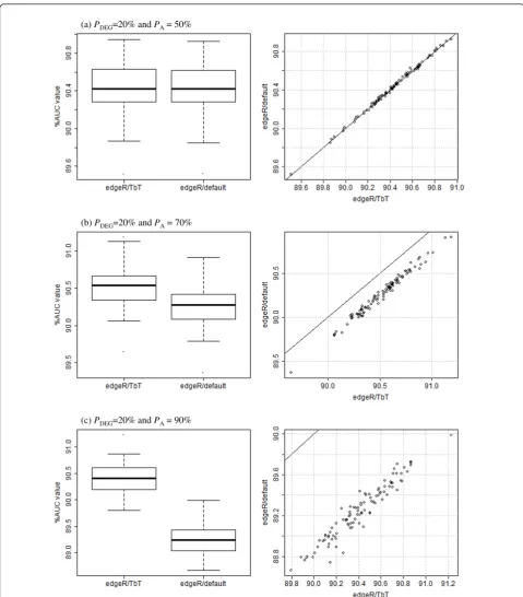
Note that different trials of simulation analysis generally yield different AUC values even if the same simulation conditions are introduced. It is important to show the statistical significance, if any, of our proposed method. The distributions of AUC values for two edgeR-related combinations (edgeR/TbT and edgeR/default) under three conditions (PA = 50, 70, and 90% with a fixed
PDEGvalue of 20%) are shown in Figure 2. The
perfor-mances between the two combinations were very similar when PA= 50% (Figure 2a; p-value = 0.95, Wilcoxon
rank sum test). This is reasonable because the average estimate of the PA values by TbT in the 100 trials
(49.62%) was quite close to the truth (i.e., 50%) and TMM uses a fixed PAvalue of 50%. The higher the PA
value (> 50%) TbT estimates, the higher the perfor-mance of TbT (compared to TMM) that can be expected.
Different from the above unbiased case (PA= 50%),
we observed the obvious superiority of TbT under the
other two conditions (PA = 70 and 90%). A significant
improvement resulting from use of TbT may seem doubtful because of the very small difference between the two average AUC values (e.g., 90.52% foredgeR/TbT and 90.26% for edgeR/default whenPA= 70%; left panel
of Figure 2b), but the edgeR/TbT combination did out-perform theedgeR/default combination in all of the 100 trials under the two conditions (right panels of Figures 2b and 2c), and the p-values were lower than 0.01 (Wil-coxon rank sum test).
Table 1 shows the average AUC values for the two edgeR-related combinations under the various simula-tion condisimula-tions (PDEG = 5-30% and PA = 50-100%).
Overall,edgeR/TbT performed better thanedgeR/default for most of the simulation conditions analyzed. The relative performance of TbT compared to the default method (i.e., the TMM method [16] in this case) can be seen to improve according to the increasedPA values
starting from 50%. This is because our estimated values for PDEG andPAare closer to the true values than the
fixed values of TMM (PDEG = 60% andPA= 50%; see
Table 2). The closeness of those estimations will inevita-bly increase the overall accuracy of assignment for DE and lead directly to the higher AUC values. This success primarily comes from our three-step normalization strategy, TbT (the TMM-baySeq-TMM pipeline).
Table 3 shows the simulation results for the other six combinations. As can be seen, TbT performed better than the individual default normalization methods implemented in the other three packages (DESeq[20], baySeq[18], andNBPSeq[21]). When we compare the results of the four default procedures (edgeR/default, DESeq/default,baySeq/default, and NBPSeq/default), the edgeR/default combination outperforms the others. This result suggests the superiority of the default normaliza-tion method (i.e., TMM) implemented in the edgeR package and the validity of our choices at steps 1 and 3 in our TbT normalization strategy. For reproducing the research, the R-code for obtaining a small portion of the above results is given in Additional file 1.
(a) PDEG=20% and PA= 50%
(b) PDEG=20% and PA= 70%
(c) PDEG=20% and PA= 90%
Figure 2Distributions of AUC values for twoedgeR-related combinations. Simulation results for 100 trials underPA= (a) 50%, (b) 70%, and
(c) 90%, withPDEG= 20%. Left panel: box plots for AUC values. Right panel: scatter plots for AUC values. When the performances between the
To mitigate this concern, we performed simulations with compatible directions of DE by adding a floor value of fold-changes (> 1.2-fold) when introducing DEGs. In this simulation, the fold-changes for DEGs were randomly
sampled from“1.2 + a gamma distribution with shape = 2.0 and scale = 0.5.”Accordingly, the minimum and mean fold-changes were approximately 1.2 and 2.2 (= 1.2 + 2.0 × 0.5), respectively. We confirmed the superiority of TbT under the various simulation conditions (PDEG= 5-30%
andPA= 50-100%) with the above simulation framework
(data not shown). An M-A plot of the simulation result whenPDEG= 20% andPA= 90% is given in Additional file
2. The R-code for obtaining the full results under the simulation condition is given in Additional file 3.
Iterative normalization approach
Recall that the outperformance of TbT compared to TMM (see Table 1 and Figure 2) is by virtue of our
Table 1 Average AUC values for twoedgeR-related combinations.
PA= 50% 60% 70% 80% 90% 100%
(a)edgeR/TbT
PDEG= 5% 90.52 89.92 90.58 90.67 90.59 90.10
10% 90.33 90.23 90.80 90.14* 91.02* 90.39*
20% 90.43 90.53 90.52* 90.60* 90.41* 90.41*
30% 90.71 90.66* 90.23* 90.67* 90.00* 89.46*
(b)edgeR/ default
5% 90.52 89.92 90.56 90.62 90.50 89.95 10% 90.33 90.21 90.73 89.99 90.74 89.89 20% 90.43 90.49 90.26 90.00 89.24 88.40 30% 90.71 90.54 89.58 89.35 87.20 84.55
Average AUC values of total of 100 trials for each simulation condition: (a) edgeR/TbT and (b)edgeR/default. Simulation data contain a total of 20,000 genes:PDEG% of genes is DEGs, andPA% ofPDEGis higher in Sample A. A
total of 24 conditions (fourPDEGvalues × sixPAvalues) are shown. Highest
AUC value for each condition is in bold. AUC values with asterisks indicate significant improvements (p-value < 0.01, Wilcoxon rank sum test).
Table 2 Estimated values forPDEGandPAby TbT.
TruePA= 50% 60% 70% 80% 90% 100%
(a) EstimatedPDEG(%)
PDEG= 5% 5.65 5.44 5.68 5.61 5.67 5.54
10% 9.38 9.39 9.58 9.28 9.54 9.31
20% 17.14 17.41 17.21 17.22 17.11 17.01 30% 25.47 25.19 24.87 25.15 24.61 24.34
(b) EstimatedPA(%)
5% 49.44 55.08 59.55 65.56 70.02 74.35 10% 50.66 56.27 61.64 67.47 73.98 79.51 20% 49.62 57.41 63.67 69.17 75.49 82.30 30% 50.05 56.58 63.34 70.08 72.47 76.05
(c) Sensitivity
5% 62.17 59.53 62.13 62.06 61.79 60.32 10% 63.61 63.41 64.85 62.59 64.27 62.31 20% 67.37 68.15 67.24 66.68 65.13 63.98 30% 71.07 70.09 68.53 68.69 63.99 59.56
(d) Specificity
5% 97.35 97.43 97.31 97.39 97.31 97.37 10% 96.70 96.67 96.62 96.69 96.60 96.64 20% 95.53 95.39 95.40 95.26 95.01 94.84 30% 94.25 94.22 94.00 93.67 92.42 90.89
(e) Accuracy
5% 95.58 95.52 95.54 95.61 95.52 95.50 10% 93.36 93.31 93.42 93.26 93.34 93.17 20% 89.86 89.90 89.73 89.50 88.99 88.62 30% 87.25 86.94 86.32 86.13 83.84 81.43
Average estimates of total of 100 trials for (a)PDEGand (b)PA. The (c)
sensitivity, (d) specificity, and (e) accuracy for the estimation are also shown.
Table 3 Average AUC values for other six combinations.
PA= 50% 60% 70% 80% 90% 100%
(a)DESeq/TbT
PDEG=
5%
85.03 83.94 85.20 85.31 85.12* 84.60*
10% 86.94 86.90 87.42* 86.80* 87.61* 86.95*
20% 89.05 89.23 89.18* 89.33* 88.97* 88.95*
30% 90.30 90.20* 89.79* 90.11* 89.44* 88.80*
(b)DESeq/default
5% 85.03 83.92 85.13 85.19 84.84 84.18 10% 86.93 86.85 87.27 86.46 87.07 86.15 20% 89.06 89.19 88.93 88.62 87.76 86.84 30% 90.30 90.00 88.94 87.95 85.36 81.98
(c)baySeq/TbT
5% 89.91 89.45 89.91* 90.17* 89.93* 89.36*
10% 89.89 89.90* 90.46* 89.79* 90.28* 90.02*
20% 90.39* 90.46* 90.40* 90.49* 90.21* 90.47*
30% 90.80 90.55* 90.44* 90.69* 89.26* 88.33*
(d)baySeq/ default
5% 89.67 89.27 88.62 88.69 86.37 86.18 10% 89.80 89.55 89.52 87.71 84.14 83.86 20% 90.22 88.78 88.92 87.85 79.09 69.65 30% 90.76 90.05 87.21 79.69 65.45 53.37
(e)NBPSeq/TbT
5% 90.75* 90.18 90.80* 90.90* 90.78* 90.33*
10% 90.59* 90.47* 91.00* 90.34* 91.14* 90.49*
20% 90.67* 90.72* 90.70* 90.68* 90.42* 90.37*
30% 90.92 90.83* 90.32* 90.74* 89.89* 89.23*
(f)NBPSeq/ default
5% 90.48 90.00 89.71 89.58 87.85 87.60 10% 90.34 90.15 90.11 88.46 86.19 85.38 20% 90.39 89.12 89.22 88.29 81.59 73.93 30% 90.84 90.26 87.45 81.96 70.97 60.73
DEG elimination strategy for normalizing tag count data and that the identification of DEGs in TbT is performed using baySeq with the TMM normalization factors at step 2. From these facts, it is expected that the accuracy of the DEG identification at step 2 can be increased by usingbaySeqwith the TbT factors instead of the TMM factors whenPA> 50%. The advanced DEG elimination
procedure (the TbT-baySeq-TMM pipeline) can produce different normalization factors (say “TbT1”) from the original ones. As also illustrated in Figure 3a, this proce-dure can repeatedly be performed until the calculated normalization factors become convergent.
The results under three simulation conditions (PA=
50, 70, and 90% with a fixed PDEGvalue of 20%) are
shown in Figures 3b-d. The left panels show the accura-cies of DEG identifications when step 2 in our DEG elimination procedures is performed using the following normalization factors: TMM (Default), TbT (First), TbT1 (Second), and TbT2 (Third). As expected, the iterative approach does not positively affect the results whenPA= 50% (Figure 3b). Indeed, the performances
between the baySeq/TMM combination (Default) and thebaySeq/TbT2 combination (Third) are not statisti-cally distinguished (p= 0.38, Wilcoxon rank sum test). Meanwhile, the use of the baySeq/TbT combination (First) can clearly increase the accuracy compared to use of thebaySeq/TMM combination (Default), though the subsequent iterations do not improve the accuracies whenPA= 70% (Figure 3c, left panel). An advantageous
trend for the iterative approach was also observed until the second iteration (Second; thebaySeq/TbT1 combina-tion) whenPA= 90% (Figure 3d, left panel).
The right panels for Figures 3b-d show the AUC values when the following normalization factors are combined with theedgeR package: TbT (Default), TbT1 (First), TbT2 (Second), and TbT3 (Third). The overall trend is the same as that of the accuracies shown in the left panels: the iterative TbT approach can outperform the original TbT approach when the degree of biased differential expression is high (PA> 50%). We confirmed
the utility of the iterative approach with the other three packages (DESeq, baySeq, and NBPSeq) (data not shown). These results suggest that the iterative approach can be recommended, especially when thePAvalue
esti-mated by the original TbT method is displaced from 50%.
Nevertheless, we should emphasize that the improvement of the iterative TbT approach compared to the original TbT approach is much smaller than that of the TbT compared to the default normalization methods implemented in the four R packages investi-gated (Figures 2 and 3). For example, the average dif-ference of the AUC values between the edgeR/TbT3 and the edgeR/TbT is 0.02% (Figure 3c) while the
average difference of the AUC values between the edgeR/TbT and the edgeR/default is 0.26% (Figure 2b), when PA = 70%. Note also that the baySeq package
used in step 2 in our TbT method is much more com-putationally intensive than the other three packages, indicating that the n times iteration of TbT roughly requires n-fold computation time. In this sense, a speed-up of our proposed DEG elimination strategy should be performed next as future work. The R-code for obtaining a small portion of the above results is given in Additional file 4.
Real data (wildtype vs.RDR6knockout dataset used in
baySeqstudy)
Finally, we show results from an analysis similar to that described in Ref. [18]. In brief, Hardcastle and Kelly compared two wildtype and two RNA-dependent RNA polymerase 6 (RDR6) knockout Arabidopsis thaliana leaf samples by sequencing small RNAs (sRNAs). From a total of 70,619 unique sRNA sequences, they identified 657 differentially expressed (DE) sRNAs that uniquely match tasRNA, which is produced by RDR6, and that are decreased in RDR6mutants and regarded as provi-sional true positives. Therefore, we assume that the logi-cal values for PDEG and PA are at least 0.93% (= 657/
70,619) and around 100%, respectively. In accordance with that study [18], the evaluation metric here is that a good method should be able to rank those true positives as highly as possible. Recall that the strategy for TbT is to normalize data after the elimination of such DE sRNAs for such a purpose.
The TbT estimated 9.0% ofPDEG(5,495potential DE
sRNAs) and 70.2% of PA. We found that the 5,495
sRNAs included 255 of the 657 true positives. This sug-gests that our strategy was effective because the original percentage (657/70,619 = 0.93%) of true positives decreased ((657 - 255)/(70,619 - 5,495) = 0.62%) before the TbT normalization factor was calculated at step 3. In summary, the TbT normalization factor was calcu-lated based on 65,124 (= 70,619 - 5,495) potentially non-DE sRNAs after 255 out of the 657 provisional DE sRNAs were eliminated.
(b)PDEG=20% and PA= 50%
(c)PDEG=20% and PA= 70%
(d) PDEG=20% and PA= 90% DefaultTbT procedure step1: TMM
step2: baySeq step3: TMM
Ļ
TbT
(a)
First iteration step1: TbT
step2: baySeq step3: TMM
Ļ
TbT1
Seconditeration step1: TbT1
step2: baySeq step3: TMM
Ļ
TbT2
Thirditeration step1: TbT2
step2: baySeq step3: TMM
Ļ
TbT3
p< 0.01 p= 0.88 p= 0.49 p= 0.61 p= 0.86 p= 0.55
p< 0.01 p< 0.01 p= 0.60
p= 0.77 p= 0.71 p= 0.89
p= 0.74 p= 1.00 p= 0.99
p= 0.04 p= 0.71 p= 0.96
Figure 3Results of iterative TbT approach. (a) Procedure for iterative TbT approach until the third iteration, and simulation results underPA=
(b) 50%, (c) 70%, and (d) 90%, withPDEG= 20%. Left panel: accuracies of DEG identifications when step 2 in our DEG elimination strategy is
(a)
(b)
Three combinations (baySeq/TbT, edgeR/TbT, and edgeR/default) outperformed theDEGseqpackage. The higher performances of these combinations were also observed from the full ROC curves (Figure 4b). The bay-Seq/TbT combination displayed the highest AUC value (74.6%), followed by edgeR/default (70.0%) andedgeR/ TbT (69.3%). Recall that theedgeR/default combination uses the TMM normalization method [16] and that the basic strategy (i.e., potential DEGs are not used) for data normalization is essentially the same as that of our TbT. This result confirms the previous findings [15,16]: poten-tial DE entities have a negative impact on data normaliza-tion, and their existences themselves consequently interfere with their opportunity to be top-ranked.
Three combinations (edgeR/default,DESeq/default, and baySeq/default) performed differently between the current study and the original one [18]. The difference for the first two combinations can be explained by the different choices for thedefaultnormalization methods. Hardcastle and Kelly [18] used a simple normalization method by adjusting the total number of reads in each library for both packages with a reasonable explanation for why the recommended method (i.e., the default method we used here) implemented in theDESeq pack-age was not used. The TMM normalization method that we used as thedefault in theedgeR package was prob-ably not implemented in the package when they con-ducted their evaluation. We found that both procedures (i.e.,edgeR andDESeq packages with library-size nor-malization) performed poorly on average (data not shown).
The difference between the current result (baySeq/ default; solid red line in Figure 4a) and the previous result (dashed red line in Figure five in Ref. [18]) might be explained by the fact that bootstrap resampling was conducted a different number of times for estimating the empirical distribution on the parameters of the NB distribution. Although the current result was obtained using 10,000 iterations of resampling as suggested in the package, we sometimes obtained a similar result to the previous one when we analyzed baySeq/default using 1,000 iterations of resampling. We therefore determined that the previous result was obtained by taking a small sample, such as 1,000 iterations. In any case, we found that those results for the baySeq/default combination with different parameter settings were overall inferior to the baySeq/TbT combination. For reproducing the research, the R-code for obtaining the results in Figure 4 and AUC values for individual combinations is given in Additional file 5.
Conclusion
We described a strategy (called TbT as an acronym for the TMM-baySeq-TMM procedure) for normalizing tag
count data. We evaluated the feasibility of TbT based on three commonly used R packages (edgeR,DESeq, and baySeq) and a recently published package NBPSeq, using a variety of simulation data and a real dataset. By com-paring the default procedures recommended in the indi-vidual packages (edgeR/default, DESeq/default, baySeq/ default, and NBPSeq/default) and procedures where our proposed TbT was used in the normalization step instead of the default normalization method (edgeR/ TbT, DESeq/TbT, baySeq/TbT, and NBPSeq/TbT), the effectiveness of TbT has been suggested for increasing the sensitivity and specificity of differential expression analysis of tag count data such as RNA-seq.
Our study demonstrated that the elimination of poten-tial DEGs is essenpoten-tial for obtaining good normalized data. In other words, the elimination of the DEGs before data normalization can increase both sensitivity and spe-cificity for identifying DEGs. Conventional approaches consisting of two steps (i.e., data normalization and gene ranking) cannot accomplish this aim in principle. The two-step approach includes the default procedures recommended in individual packages (edgeR/default, DESeq/default, baySeq/default, and NBPSeq/default). Our proposed approach consists of a total of four steps (data normalization, DEG identification, data normaliza-tion, and DEG identification). This procedure enables potential DEGs to be eliminated before the second nor-malization (step 3).
Our TbT normalization strategy is a proposed pipeline for the first three steps, where the TMM normalization method is used at steps 1 and 3 and the empirical Baye-sian method implemented in thebaySeqpackage is used at step 2. This is because our strategy was originally designed to improve the TMM method, the default method implemented in theedgeRpackage. As demon-strated in the current simulation results comparing two groups (for example, samples A and B), the use of default normalization methods implemented in the existing R packages performed poorly in simulations where almost all the DEGs are highly expressed in Sam-ple A (i.e., the case of PA > > 50% when the range is
defined as 50% ≤ PA ≤ 100%). Although the negative
impact derived from such biased differential expression gradually increases according to the increased propor-tion of DEGs in the data, our strategy can eliminate some of those DEGs before data normalization (Tables 1, 2, and 3). The use of the empirical Bayesian method implemented in the baySeq package primarily contri-butes to solving this problem.
between compared conditions in the corresponding ChIP-seq analysis, in a similar way to theRDR6 case. We observed relatively high performances for NBPSeq/ TbT when analyzing simulation data (Tables 1 and 3) and baySeq/TbT when analyzing a real dataset (Figure 4). However, this might simply be because the simula-tion and real data used in this study were derived from the NBPSeq study [21] and the baySeq study [18], respectively. In this sense, the edgeR/TbT combination might be suitable because it performed comparably to the individual bests. The DEG elimination strategy we proposed here could be applied for many other combi-nations of methods, e.g., the use of an exact test for NB distribution [22] for detecting potential DEGs at step 2. A more extensive study with other recently proposed methods (e.g., Ref. [27]) based on many real datasets should still be performed.
Methods
All analyses were basically performed using R (ver. 2.14.1) [19] and Bioconductor [28].
Simulation details
The negative binomially distributed simulation data used in Tables 1, 2, and 3 and Figures 1, 2, and 3 were pro-duced using an R generic functionrnbinom. Each data-set consisted of 20,000 genes × 6 samples (3 of Sample A vs. 3 of Sample B). Of the 20,000 genes, the PDEG %
were DEGs at the four-fold level, andPA% of thePDEG
% was higher in Sample A. For example, the simulation condition for Figure 1 used 20% of PDEGand 90% of PA,
giving 4,000 (= 20,000 × 0.20) DEGs, 3,600 (= 20,000 × 0.20 × 0.9) of which are highly expressed in Sample A in the simulation dataset.
The variance of the NB distribution can generally be modelled asV=μ+jμ2. The empirical distribution of read counts for producing the mean (μ) and dispersion (j) parameters of the model was obtained from Arabi-dopsis data (three biological replicates for both the trea-ted and non-treatrea-ted samples) in Ref. [21]. The simulations were performed using a total of 24 combi-nations ofPDEG(= 5, 10, 20, and 30%) andPA(= 50, 60,
70, 80, 90, and 100%) values. The full R-code for obtain-ing the simulation data is described in Additional file 1. The parameter param1in Additional file 1 corresponds to the degree of fold-change.
Simulations with different types of DEG distribution were also performed in this study. The fold-change values for individual genes were randomly sampled from a gamma distribution with shape and scale para-meters. Specifically, an R generic function rgamma with respective values of 2.0 and 0.5 for the shape and scale parameters was used. This roughly gives respec-tive values of 0.0 and 1.0 for the minimum and mean
fold-changes. We added an offset value of 1.2 to pre-vent low fold-changes for introduced DEGs, giving respective values of 1.2 and 2.2 for the minimum and mean fold-changes. The full R-code for obtaining the simulation data is described in Additional file 3. The values in param1 in Additional file 3 correspond to those parameters.
Wildtype vs.RDR6knockout dataset used inbaySeqstudy The dataset was obtained by e-mail from the author of Ref. [18]. The dataset (named“rdr6_wt.RData”) consists of 70,619 sRNAs × 4 samples (2 wildtype and 2 RDR6 knockout samples). Of the 70,619 sRNAs, 657 were used as true DE sRNAs whose expressions were higher in the wildtype than theRDR6knockout samples.
Gene ranking with default procedure
Ranked gene lists according to the differential expres-sion are pre-required for calculating AUC values. The input data for differential expression analysis using five R packages (edgeR ver. 2.4.1, DESeq ver. 1.6.1, baySeq ver. 1.8.1, NBPSeqver. 0.1.4, and DEGseq ver. 1.6.2) is basically the raw count data where each row indicates the gene (or transcript), each column indicates the sam-ple (or library), and each cell indicates the number of reads mapped to the gene in the sample. The execution of thebaySeq package was performed using data after scaling for RPM mapped reads.
The analysis using the edgeR packages with default settings (i.e., theedgeR/default combination) was per-formed using four functions (calcNormFactors, estimate-CommonDisp, estimateTagwiseDisp, and exactTest) in the package [17]. The TMM normalization factor can be obtained from the output object after applying the calc-NormFactors function [16]. The genes were ranked in ascending order of thep-values.
TheDESeq/default combination was performed using three functions (estimateSizeFactors,estimateDispersions, and nbinomTest) in the package. The genes were ranked in ascending order of thep-values adjusted for multiple-testing with the Benjamini-Hochberg procedure.
TheNBPSeq/default combination was performed using the nbp.test function in the package [21]. The genes were ranked in ascending order of the p-values of the exact NB test.
The analysis using theDEGseqpackage [26] was per-formed for benchmarking the current study and a pre-vious study [18], both of which analyzed the same real dataset. There are multiple methods in the DEGseq package [26]. Following from the previous study, we used an MA plot-based method with random sampling (MARS), i.e., the DEGexp function with method = “MARS” option was used. A higher absolute value for the statistics indicates a higher degree of differential expression. Accordingly, the genes were ranked in des-cending order of the absolute value. Note that the execution of this package (ver. 1.6.2) was performed using R 2.13.1 because we encountered an error when executing the more recent version (ver. 1.8.0) using R 2.14.1.
TbT normalization strategy
Our proposed strategy is an analysis pipeline consisting of three steps. In step 1, the TMM normalization factors are calculated by using thecalcNormFactorsfunction in theedgeR package with the raw count data. These fac-tors are used for calculating effective library sizes, i.e., library sizes multiplied by the TMM factors.
In step 2, potential DEGs are identified by using the baySeq package with the RPM data. Different from the above baySeq/default combination, the analysis is per-formed using the effective library sizes. The effective library sizes are introduced when constructing a count-Data object, the input data for thegetPriors.NB func-tion. By applying the subsequent getLikelihoods.NB function, the percentage of DEGs in the data (the PDEG
value) and the corresponding potential DEGs can be obtained.
In step 3, TMM normalization factors are again calcu-lated based on the raw count data after eliminating the estimated DEGs. The TbT normalization factors are defined as (the TMM normalization factors calculated in this step) × (library sizes after eliminating the DEGs)/ (library sizes before eliminating the DEGs). As the TbT normalization factors are comparable with the original TMM normalization factors such as those calculated in step 1, effective library sizes can also be calculated by multiplying library sizes by the TbT factors.
The four combinations coupled with the TbT normal-ization strategy (edgeR/TbT,DESeq/TbT,baySeq/TbT, andNBPSeq/TbT) were analyzed to compare the above four combinations coupled with the default normaliza-tion strategy. The edgeR/TbT combination introduced the TbT normalization factors instead of the original
TMM factors. The NBPSeq/TbT combination
introduced the TbT normalization factors in thenbp.test function. The remaining two combinations (DESeq/TbT and baySeq/TbT) introduced the effective library sizes, i. e., the original library sizes multiplied by the TbT factors.
Additional material
Additional file 1: R-code for simulation analysis. After execution of this R-code with default parameter settings (i.e.,rep_num= 100,param1
= 4,.., andparam6= 090), two output files named“Fig1.png”and
“resultNB_020_090.txt”can be obtained. The former is the same as Figure 1. The latter output file will contain raw data for Tables 1, 2, 3 whenPDEG
= 20% andPA= 90%. The numbers given asrep_num,param1,..., and
param6indicate the number of trials (rep_num), degree of differential expression of fold-change (param1-fold), number of libraries for sample A (param2), number of libraries for sample B (param3), total number of genes (param4), truePDEG(param5), and truePA(param6), respectively.
Accordingly, for example, respective values forparam5andparam6
should be changed to“030”and“060”, to obtain the raw results when
PDEG= 30% andPA= 60%.
Additional file 2: Result of TbT using simulation data with > 1.2-fold of DEGs. Legends in this figure are essentially the same as those described in Figure 1. The difference between the two is the distributions of DEGs (magenta dots). This simulation does not have DEGs with low fold-changes (< = 1.2-fold) and the average fold-change is theoretically 2.2. The R code for obtaining the full results under the simulation condition (i.e.,PDEG= 20% andPA= 90%) is given in
Additional file 3.
Additional file 3: R-code for obtaining simulation results with > 1.2-fold of DEGs. After execution of this R-code with default parameter settings (i.e.,rep_num= 100,param1= c(1.2, 2.0, 0.5),..., andparam6= 090), two output files named“Additional2.png”and“resultNB2_020_090. txt”can be obtained. The former is the same as Additional file 2. The format of the latter output file is essentially the same as the
“resultNB_020_090.txt”file obtained by executing Additional file 1. The main difference between the current code and Additional file 1 is in the parameter settings for producing the distributions of DEGs atparam1. The parameter values (1.2, 2.0, and 0.5) indicated inparam1are used for the minimum change (= 1.2) and for random sampling of fold-change values from a gamma distribution with shape (= 2.0) and scale (= 0.5) parameters, respectively.
Additional file 4: R-code for obtaining raw results shown in Figure
3. After execution of this R-code with default parameter settings (i.e.,
rep_num= 100,param1= 4,..., andparam7= 5000), four output files named“iteration0_020_090.txt”,“iteration1_020_090.txt”,
“iteration2_020_090.txt”, and“iteration3_020_090.txt”can be obtained. The box plots forDefault,First,Second, andThirdshown in Figure 3 are produced using values in two columns (named“accuracy”and“AUC (edgeR/TbT)”) in the first, second, third, and fourth file, respectively. The
p-values were calculated based on the Wilcoxon rank sum test.
Additional file 5: R-code for producing Figure4and AUC values for individual combinations. We obtained an input file (named“rdr6_wt. RData”) from Dr. T.J. Hardcastle (the corresponding author of Ref. [18]). After execution of this R-code, three output files (arbitrarily named
“Fig4a.png”,“Fig4b.png”, and“AUCvalue_Fig4b.txt”) can be obtained.
List of abbreviations used
DE: differential expression; DEG: differentially expressed gene; EB: embryonic body; RPM: reads per million (normalization); sRNA: small RNA; tasRNA:TAS
locus-derived small RNA; TMM: trimmed mean of M values (method).
Acknowledgements
The authors thank Dr. TJ Hardcastle for providing the dataset used in the
24500359 to KK and 22128008 to TN) from the Japanese Ministry of Education, Culture, Sports, Science and Technology (MEXT).
Author details
1
Agricultural Bioinformatics Research Unit, Graduate School of Agricultural and Life Sciences, The University of Tokyo, 1-1-1 Yayoi, Bunkyo-ku, Tokyo 113-8657, Japan.2Project on Health and Anti-aging, Kanagawa Academy of Science and Technology, 3-2-1 Sakado, Takatsu-ku, Kawasaki, Kanagawa 213-0012, Japan.3Advanced Science Research Center, Kanazawa University, 13-1 Takara-machi, Kanazawa 920-0934, Japan.
Authors’contributions
KK performed analyses and drafted the paper. TN provided helpful comments and refined the manuscript. KS supervised the critical discussion. All the authors read and approved the final manuscript.
Competing interests
The authors declare that they have no competing interests.
Received: 1 December 2011 Accepted: 5 April 2012 Published: 5 April 2012
References
1. Weber AP, Weber KL, Carr K, Wilkerson C, Ohlrogge JB:Sampling the Arabidopsis transcriptome with massively parallel pyrosequencing.Plant Physiol2007,144(1):32-42.
2. Mardis ER:The impact of next-generation sequencing technology on genetics.Trends Genet2008,24(3):133-141.
3. Schena M, Shalon D, Davis RW, Brown PO:Quantitative monitoring of gene expression patterns with a complementary DNA microarray.
Science1995,270(5235):467-470.
4. Lockhart DJ, Dong H, Byrne MC, Follettie MT, Gallo MV, Chee MS, Mittmann M, Wang C, Kobayashi M, Horton H, Brown EL:Expression monitoring by hybridization to high-density oligonucleotide arrays.Nat Biotechnol1996,14(13):1675-1680.
5. Asmann YW, Klee EW, Thompson EA, Perez EA, Middha S, Oberg AL, Therneau TM, Smith DI, Poland GA, Wieben ED, Kocher JP:3’tag digital gene expression profiling of human brain and universal reference RNA using Illumina Genome Analyzer.BMC Genomics2009,10:531. 6. Oshlack A, Wakefield MJ:Transcript length bias in RNA-seq data
confounds systems biology.Biology Direct2009,4:14.
7. Mortazavi A, Williams BA, McCue K, Schaeffer L, Wold B:Mapping and quantifying mammalian transcriptomes by RNA-Seq.Nat Methods2008, 5(7):621-628.
8. Sultan M, Schulz MH, Richard H, Magen A, Klingenhoff A, Scherf M, Seifert M, Borodina T, Soldatov A, Parkhomchuk D, Schmidt D, O’Keeffe S, Haas S, Vingron M, Lehrach H, Yaspo ML:A global view of gene activity and alternative splicing by deep sequencing of the human transcriptome.Science2008,321(5891):956-960.
9. Trapnell C, Williams BA, Pertea G, Mortazavi A, Kwan G, van Baren MJ, Salzberg SL, Wold BJ, Pachter L:Transcript assembly and quantification by RNA-Seq reveals unannotated transcripts and isoforms switching during cell differentiation.Nat Biotechnol2010,28:511-515.
10. Lee S, Seo CH, Lim B, Yang JO, Oh J, Kim M, Lee S, Lee B, Kang C, Lee S: Accurate quantification of transcriptome from RNA-Seq data by effective length normalization.Nucleic Acids Res2010,39(2):e9.
11. Nicolae M, Mangul S, Mandoiu II, Zelikovsky A:Estimation of alternative splicing isoform frequencies from RNA-Seq data.Algorithms Mol Biol2011, 6:9.
12. Cloonan N, Forrest AR, Kolle G, Gardiner BB, Faulkner GJ, Brown MK, Taylor DF, Steptoe AL, Wani S, Bethel G, Robertson AJ, Perkins AC, Bruce SJ, Lee CC, Ranade SS, Peckham HE, Manning JM, McKernan KJ, Grimmond SM: Stem cell transcriptome profiling via massive-scale mRNA sequencing.
Nat Methods2008,5(7):613-619.
13. Marioni JC, Mason CE, Mane SM, Stephens M, Gilad Y:RNA-seq: an assessment of technical reproducibility and comparison with gene expression arrays.Genome Res2008,18(9):1509-1517.
14. Balwierz PJ, Carninci P, Daub CO, Kawai J, Hayashizaki Y, Van Belle W, Beisel C, van Nimwegen E:Methods for analyzing deep sequencing expression data: contructing the human and mouse promoteome with deepCAGE data.Genome Biol2009,10(7):R79.
15. Bullard JH, Purdom E, Hansen KD, Dudoit S:Evaluation of statistical methods for normalization and differential expression in mRNA-Seq experiments.BMC Bioinformatics2010,11:94.
16. Robinson MD, Oshlack A:A scaling normalization method for differential expression analysis of RNA-seq data.Genome Biol2010,11:R25. 17. Robinson MD, McCarthy DJ, Smyth GK:edgeR: a Bioconductor package
for differential expression analysis of digital gene expression data.
Bioinformatics2010,26(1):139-140.
18. Hardcastle TJ, Kelly KA:baySeq: empirical Bayesian methods for identifying differential expression in sequence count data.BMC Bioinformatics2010,11:422.
19. R Development Core Team:R: A Language and Environment for Statistical Computing.R Foundation for Statistical computing, Vienna, Austria; 2011.
20. Anders S, Huber W:Differential expression analysis for sequence count data.Genome Biol2010,11:R106.
21. Di Y, Schafer DW, Cumbie JS, Chang JH:The NBP negative binomial model for assessing differential gene expression from RNA-Seq.Stat Appl Genet Mol Biol2011,10:art24.
22. Robinson MD, Smyth GK:Small-sample estimation of negative binomial dispersion, with applications to SAGE data.Biostatistics2008,9:321-332. 23. Kadota K, Nakai Y, Shimizu K:A weighted average difference method for
detecting differentially expressed genes from microarray data.Algorithms Mol Biol2008,3:8.
24. Kadota K, Nakai Y, Shimizu K:Ranking differentially expressed genes from Affymetrix gene expression data: methods with reproducibility, sensitivity, and specificity.Algorithms Mol Biol2009,4:7. 25. Kadota K, Shimizu K:Evaluating methods for ranking differentially
expressed genes applied to MicroArray Quality Control data.BMC Bioinformatics2011,12:227.
26. Wang L, Feng Z, Wang X, Wang X, Zhang X:DEGseq: an R package for identifying differentially expressed genes from RNA-seq data.
Bioinformatics2010,26(1):136-138.
27. Bergemann TL, Wilson J:Proportion statistics to detect differentially expressed genes: a comparison with log-ratio statistics.BMC Bioinformatics2011,12:228.
28. Gentleman RC, Carey VJ, Bates DM, Bolstad B, Dettling M, Dudoit S, Ellis B, Gautier L, Ge Y, Gentry J, Hornik K, Hothorn T, Huber W, Iacus S, Irizarry R, Leisch f, Li C, Maechler M, Rossini AJ, Sawitzki G, Smith C, Smyth G, Tierney L, Yang JY, Zhang J:Bioconductor: open software development for computational biology and bioinformatics.Genome Biol2004,5:R80.
doi:10.1186/1748-7188-7-5
Cite this article as:Kadotaet al.:A normalization strategy for comparing tag count data.Algorithms for Molecular Biology20127:5.
Submit your next manuscript to BioMed Central and take full advantage of:
• Convenient online submission
• Thorough peer review
• No space constraints or color figure charges
• Immediate publication on acceptance
• Inclusion in PubMed, CAS, Scopus and Google Scholar
• Research which is freely available for redistribution