Identification Of Interplanetary Coronal Mass Ejection With Magnetic Cloud In Year 2005 At 1 AU

Identification Of Interplanetary Coronal Mass

Ejection With Magnetic Cloud In Year 2005 At 1

AU

D.S.Burud, R .S. Vhatkar, M. B. Mohite

Abstract: Coronal mass ejection (CMEs) propagate in to the interplanetary medium are called as Interplanetary Coronal Mass Ejection (ICME). A set of signatures in plasma and magnetic field is used to identify the ICMEs. Magnetic Cloud (MC) is a special kind of ICMEs in which internal magnetic field configuration is similar like flux rope. We have used the data obtained from ACE Advance Composition Explorer (ACE) based in-situ measurements of Magnetic Field Experiment (MAG) and Solar Wind Electron, Proton and Alpha Monitor (SWEPAM) experiment for the data of magnetic field and plasma parameters respectively. The magnetic field data and plasma parameters of ICMEs used to distinguish them as magnetic cloud, non magnetic cloud. We analyzed eighteen ICMEs observed during January 2005 to December 2005, which is the beginning of declining phase of solar cycle 23. The analysis of magnetic field in the frames of the flux ropes like structure using a Minimum Variance Analysis (MVA) method, and have identified 30% ICMEs in the year 2005, which shows magnetic field rotation in a plane and confirmed as ICMEs with MCs.

Keywords: magnetic cloud (MC), interplanetary coronal mass ejection (ICME), minimum variance analysis (MVA).

————————————————————

Introduction:-

Coronal mass ejections (CMEs) are an energetic phenomenon originated in the Sun‘s corona, CMEs are eruptions of plasma and magnetic fields that drive space weather in the near-Earth environment. CMEs are extremely dynamical huge events in which the plasma, initially contained in closed coronal magnetic field lines, is ejected into interplanetary space. CMEs are now well known to be the cause of intense geomagnetic storms that affects the space weather in the near-Earth environment. CMEs were firstly observed in 1970 with the help of coronograph (OSO-7 and Skylab). From 1996 Solar Heliosphere Observatory (SOHO) providing solar coverage and data for CMEs which is as follows:-

 Speeds varying from 50 to more than 2000 km/s.

 Angular widths from a few degrees up to 360°

 More than 3 events (on average) are observed

per day during solar maximum.

 During solar minimum CMEs are originating close to

the equator and occur, on average less than once per day.

 Ejected mass from 5 to 50 billion tons

 Energies between 1023 and 1024 J

An ICME is simply the interplanetary manifestation of a CME. Some ICMEs drive shocks in interplanetary space, but these are not identified in coronagraph data. ICMEs are detected by following set of signatures :- (description

applies to ∼1 AU heliospheric distance)

o The magnetic field (B)

o Plasma dynamics (P)

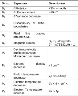
Table No: 1 Signatures used to identify ICMEs in the

Heliosphere

All signatures described in table no. 1 were not observed in single ICME. Few of them were presented in each ICME. It was not necessary that all signatures described in table no.1 must have to be observed in each and every ICME. Some portions of ICME show certain signatures and other portion of the same structure shows different signatures as mentioned in table no. 1. Even if few signatures were absent the structure will be still remains as ICME. From this we concluded that, these all signatures were not sufficient to identify an ICME present in solar wind. Because of these reasons, the identification of ICMEs in solar wind plasma

Sr.no. Signature Description

B1 B Rotation ≥30◦, smooth

B2 B Enhancement >10 nT

B3 B Variance decrease

B4

Discontinuity at ICME boundaries

B5

Field line draping

around ICME

B6 Magnetic clouds

B1, B2 along with

β=_nkTB2/(2μ0) < 1

P1

Declining velocity profile/expansion Monotonic decrease

P2

Extreme density

decrease ≤1 cm

−3

P3

Proton temperature

decrease Tp < 0.5Texp

P4

Electron temperature

decrease Te < 6 × 10

4 K

P5

Electron Temperature

increase Te >Tp

_____________________________

 Miss- dipali burud, Shivaji University Kolhapur-416004,India PH-07304018250.

 E-mail: [email protected]

271

and magnetic field data is still ‗something of an art‘ [1].

Boundary determination of ICME is also a difficult task. Signatures do not normally correlate exactly in time and space. Start and end of the events depends chosen certain signature. We had used presence of low proton temperature signature to identify the ICME event in this paper. Magnetic clouds (MCs) are a subset of interplanetary coronal mass ejections (ICMEs), typically identified, at least initially, by three main criteria used to identify the MC are as following [2].

 The magnetic field rotates smoothly over a large

angle during an interval of the order of one day

 The magnetic field strength is higher than in the

typical solar wind

 The proton temperature is lower than in the typical

solar wind [3], [4].

Fig.1: Magnetic field configuration inside a MC. From [5]

The magnetic field inside a MC consists of twisted helical lines with decreasing angle between the helical lines and the axial field, from the edges to the center (as shown in fig.1). So that smooth magnetic field rotation is observed in magnetic field data as the spacecraft is immersed in the cloud. MC is interplanetary manifestation of solar flux ropes (as show in fig. 1).

Minimum

variance

analysis

and

data

analysis[1-18] :-

For studies of magnetic fields in space, minimum-variance analysis (MVA) has been used to identify the magnetic field rotation, one dimensional discontinuity in magnetic field data. It helps in identifying the directions of minimum,

medium and maximum variance of the magnetic field.

Minimum variance analysis (MVA) based on the fact that the normal is the direction of smallest variations of the

magnetic field (that is B is a constant). Normal is the

direction in which the variation in magnetic field or in mass flux must be minimum. The MVA technique is based on the Maxwell's equation

∇. 𝐵 = 0

It means that the magnetic field must be divergence free.

𝜎2 ₌1

𝑁 𝐵𝑖. 𝑛−< 𝐵 >. 𝑛

𝑁

𝑖=1 (1)

Minimum variance of the field can be calculated by using equation (1).

Where,

𝐵𝑖_{=individual field measurements}

< 𝐵 >= 1/𝑁 𝑁 𝐵𝑖

𝑖=1 = average value of the N field

measurements. n= normal unit vector N= number of data points

Using a Lagrange multiplier λ the minimization of σ² with the constraint |n| = 1 can be formulated as an eigenvalue problem:

𝑀𝐵_{𝑛 = 𝑛𝜆}

Where,

MB is the magnetic covariant matrix which reads in

component form

𝑀𝜇𝑣𝐵 =< 𝐵𝜇 >< 𝐵𝑢 > −< 𝐵𝑣>< 𝐵𝜇 >

The all λ values are the eigenvalues 𝜆₁≥ 𝜆₂≥ 𝜆₃ of MB.

Since MB is symmetric all eigenvalues are real with

eigenvectors x1, x2 and x3 are orthogonal [6]. The three

eigenvectors represent the direction of maximum,

intermediate and minimum variance of the field component

along each vector and the corresponding eigenvalues λ1, λ2

and λ3 represent the actual variances in those field

components and are therefore non-negative. The

eigenvector x3, corresponding to the smallest eigenvalue λ3

and it represents the variance of the magnetic field component along the estimated normal. MVA gives the magnetic field rotation for certain selected structures. This is the one of the condition used to identify magnetic cloud. The normal direction (n) in this case is the direction perpendicular to the plane of the rotation, since this is the direction of minimum variance of the field. In this way, the MVA provides an aid to the simple eye inspection of the magnetic field data. In application to actual observations, this condition would mean the minimum variance of the magnetic field along the normal. Then, MVA applies the eigenvalue analysis technique to the variance-covariance matrix of the magnetic field and determines such a direction. There are certain conditions which must be obeyed in order to consider the analysis as valid :

𝜆2

𝜆1≥ 2 (2)

The ratios of the Eigen values corresponding to the direction of medium and minimum variance must be higher than two. This condition implies that the ellipsoid defined by Equation (1) degenerates into an ellipsoid of revolution [18] (no significance difference between the directions of minimum and medium variance). The clear visualization of magnetic field rotation is obtained by plotting hodograms (or magnetic hodographs).

Data collection:

5 6 7 8 9 10 11 0

5 10 15 20 250 100000 200000 300000 0 10 20 30 300 400 500 600 700 800 0.00 0.02 0.04 0.06 0.08 0.10 0.12-5 0 5 10 -20 0 20 -20 -100 10 20

B

day

(a)

T (b)

N (c)

V

(d)

a

lp

h

a

/p

ro

to

n (e)

Bx

(f)

By

(g)

Bz

(h)

are from (ACE/SWEPAM) solar wind electron, proton, and alpha monitor is obtained for the year 2005. These events may include both magnetic clouds and non-cloud ejecta. Present study include eighteen ICMEs observed between January 2005 to December 2005 out of thirteen events of CME recognized by Richardson-Cane and is available online. Selection of eighteen ICMEs is based on the visual inspection of low proton temperature criteria. The data for

plasma parameters was obtained from the from

NASA/Goddard Space Flight center, space data facility

center (from the website ―Omniweb.gsfc.nasa.gov‖). This

data is obtained for hourly intervals for the plasma parameters such as speed, density, magnitude of average interplanetary magnetic field component, temperature, alpha to proton density ratio, magnetic field component in x direction (Bx), magnetic field component in y direction (By), magnetic field component in z direction (Bz). The magnetic field data is obtained from the magnetic field experiment (MAG) on board of advanced composition explorer (ACE) for sixteen seconds level two for different plasma parameters such as magnetic field component in x direction (Bx), magnetic field component in y direction (By), magnetic field component in z direction (Bz).

Data analysis:-

We performed minimum variance analysis for the assurance of all magnetic clouds in our data set must have to fulfill the conditions as per the definition of MC [4], having

a smooth rotation of magnetic field on a plane.

ICME of 7

January 2005:

The variations in plasma parameters and magnetic field

parameters of ICME observed on 7th January 2005 are as

shown in figure 2. The plots contain the data for the day 5 to11 day of the year 2005 as observed by ACE spacecraft at a distance of 1AU of CME. In the graph (a) total magnetic field strength B (nT) has been significantly enhanced with respect to the ambient magnetic field. In graph (b) shows variation of proton temperature with respect to time, the ejecta interval, according to the low proton temperature criterion [9,10], is marked with vertical solid lines. In graph (c), significant increase in density is observed suddenly as time progressed. In graph (d), as time increases speed (km/sec) decreases continuously but slowly. In graph (e), alpha to proton density ratio increases with respect to time but not exceed than 0.08. In graph(f), (g), (h) we observed total reversal of magnetic field component that is Bx, By, Bz respectively as time progressed. It shows the rotation of magnetic field component.The vertical solid line indicates the start and end time of MC based on the above described criteria and this time period is used for further analysis. For the comparison of magnetic cloud parameter with ambient solar wind parameter we had choose the approximately

same period before and after MC event. Hodograms of

MC are illustrated in fig. 3.a, 3.b and 3.c[15,16].The hodogram for intermediate to maximum variance is as observed in fig. 3.a, maximum variance is greater than

intermediate variance that is λ1=208.696 and λ2=57.48.The

variation of the magnetic field in the direction of minimum variance (min. var.) is much smaller than the direction of maximum variance (max. var.) as observed in graph 3.b.The eigen value having large magnitude difference for the case maximum variance than minimum variance that

is 𝜆1=208.696 and.Fig.3.c is hodogram of

intermediate variance against minimum variance this graph shows plane rotation of magnetic field on a plane. Moreover, the error criteria of the minimum variance

method [3] (𝜆2

𝜆1≥

2); λ2 and λ3 correspond to the Eigen

values of the directions of intermediate and minimum

variance) was satisfied that is 𝜆2

𝜆₃=4.44, which is one of the

mast important condition for magnetic field rotation is confined to a plane.

Fig.2: Plasma and magnetic field parameters of the ejecta

observed during days 5-11 of year 2005

-30 -25 -20 -15 -10 -5 0 5 10 15 20 25 30 -30

-25 -20 -15 -10 -5 0 5 10 15 20 25 30

in

te

r.

va

r.

max. var.

-30 -25 -20 -15 -10 -5 0 5 10 15 20 25 30 -30

-25 -20 -15 -10 -5 0 5 10 15 20 25 30

mi

n

.

va

r.

273

Fig. 3.c

Fig.3.a,b,c: Magnetic hodogram diagrams for day 7.6 to 8.1

day of year 2005 ICME of 14th July 2005:

Fig. (4) shows the plasma and magnetic field parameters of the ejecta observed during days 195 to 204 of year 2005 component as time continues. In graph (a) the total magnetic field strength has been decreases as time goes on increasing. In graph (b) proton temperature against time at the ejecta interval, according to the low proton temperature criterion is marked with vertical solid lines. In graph (c), decrease in density is observed as time continues. In graph (d), speed decreases continuously as time increases. In fig. (e), alpha to proton density ratio shows abrupt increment with respect to time. In graph (f), (g), (h) we do not observed total reversal of magnetic field component as time progressed. No rotation of magnetic field component is observed. Magnetic field hodogram diagram for ejecta is as shown in fig. 5.a, 5.b, 5.c [15,16].The hodograms intermediate against minimum (shown in fig. 5.a). The variation of the magnetic field in the direction of minimum variance (min. var.) is much larger than the direction of maximum variance (max. var.), as shown in hodogram 5.b, the eigenvalue having small magnitude difference for the maximum variance than

minimum variance that is λ1=23.52 and λ3=7.938. hodogram

of minimum verses intermediate (see fig. 5.c) shows large variation and no rotation in field direction is observed on a plane. Moreover, the error criteria of the minimum variance method [3]

𝜆2

𝜆3≥ 2 ; 𝜆2 and 𝜆3correspond to the eigenvalues of the

directions of intermediate and minimum variance was not satisfied 𝜆2

𝜆3= 1.74, which means that the magnetic field

rotation is not confined to a plane.

Fig. 4: Plasma and magnetic field parameters of the ejecta

observed during days 195-204 of year 2005.

Fig. 5.a Fig.5.b

Fig.5.c

Fig.5.a,b,c: Magnetic hodogram diagrams for day195 to

204 day of year 2005.

-15 -10 -5 0 5 10 15

-15 -10 -5 0 5 10 15

in

te

r.

va

r.

min. var.

195 196 197 198 199 200 201 202 203 204 0

5 10 15 0 200000 4000000 10 20 30 300 400 500 600 0 10 20 -10-5 0 5 10 -10 0 10 -10 0 10

B

day

(a)

T (b)

N (c)

V (d)

a

lp

h

a

/p

ro

to

n

(e)

Bx

(f)

By (g)

Bz

(h)

-15 -10 -5 0 5 10 15

-15 -10 -5 0 5 10 15

mi

n

.

va

r.

max. var.

-15 -10 -5 0 5 10 15

-15 -10 -5 0 5 10 15

in

te

r.

va

r.

max. var. -30 -25 -20 -15 -10 -5 0 5 10 15 20 25 30

-30 -25 -20 -15 -10 -5 0 5 10 15 20 25 30

in

te

r.

va

r.

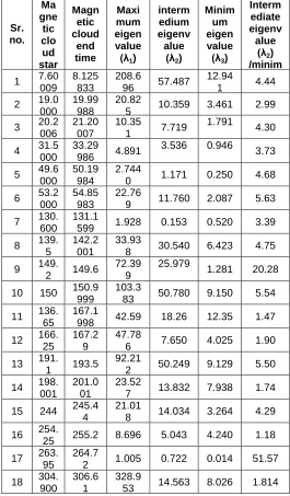
Similarly the analysis of other events listed in table no.2,the outcomes of the analysis had been summarized in table no. 2. The column first and second of this table is the start time of magnetic cloud which has observed from the graphs of the various plasma parameters, specially depends upon the low temperature criteria. By using sixty four second data from MAG/ACE for the same period we construct covariance matrix and obtain the three eigenvalues which

are summarized in column 3, 4, 5 ( λ1 ≥ λ2 ≥λ3) of table no. 2

.The condition given by equation no. 2 had been verified for

eighteen events and result is as shown in column 6 in table

no.3. The hodograms are plotted to observe variation of the magnetic field in the direction and the rotation of magnetic field on a plane.

Result and analysis:-

Total 30 ICMEs are observed in year 2005 acording to the

Richardson Cane list [6]. We have selected eighteen ICMEs

for this study by observing the low proton temperature

criteria. ICMCs are getting expand as they propagate into

interplanetary space so speed, density, proton temperature, average magnetic field were decreases as time progresses. The maximum variance direction obtained from the minimum variance analysis technique by performing covariance matrix for sixty four seconds level

Table no.2: outcome of minimum variance analysis

Two data of magnetic field for each event. The field rotation in a plane is confided by rotating observing the hodograms. From selected eighteen ICMEs (refer table no 2) it is observed that nine ICMEs According to minimum variance analysis shows rotation of magnetic field in an elliptical plane. Plasma parameter shows decrease such as speed, temperature, density etc. Magnetic field component in x, y, and z direction shows complete reversal. Thirteen ICME (in table no. 2) satisfy the error criteria:

λ2 / λ1 ≥2.

All of ICME which satisfy these criteria were not showing rotation of magnetic field on a plane as per the hodorgam observations. Only nine ICME from table no.2 shows plane of rotation and classified as magnetic cloud as described in the definition of magnetic cloud [3,4]. Remaining ICMEs do not shows magnetic field rotation in a plane even if it satisfy

the error criteria and shows both small‐ scale, large‐ scale

Sr. no.

Ma gne tic clo ud star t tim

e

Magn etic cloud

end time

Maxi mum eigen value

(λ1)

interm edium eigenv

alue

(λ2)

Minim um eigen value

(λ3)

Interm ediate eigenv alue

(λ2)

/minim um eigenv

alue

(λ3)

1 7.60

009 3

8.125 833

208.6

96 57.487

12.94

1 4.44

2 19.0

000 7

19.99 988

20.82

5 10.359 3.461 2.99

3 20.2

006 3

21.20 007

10.35

1 7.719

1.791 _4.30

4 31.5

000 5

33.29

986 4.891

3.536 0.946

3.73

5 49.6

000 2

50.19 984

2.744

0 1.171 0.250 4.68

6 53.2

000 1

54.85 983

22.76

9 11.760 2.087 5.63

7 130.

600

131.1

599 1.928 0.153 0.520 3.39

8 139.

5

142.2 001

33.93

8 30.540 6.423 4.75

9 149.

2 149.6

72.39 9

25.979

1.281 20.28

10 150 150.9

999

103.3

83 50.780 9.150 5.54

11 136.

65

167.1

998 42.59 18.26 12.35 1.47

12 166.

25

167.2 9

47.78

6 7.650 4.025 1.90

13 191.

1 193.5

92.21

2 50.249 9.129 5.50

14 198.

001

201.0 01

23.52

7 13.832 7.938 1.74

15 244 245.4

4

21.01

8 14.034 3.264 4.29

16 254.

25 255.2 8.696 5.043 4.240 1.18

17 263.

95

264.7

2 1.005 0.722 0.014 51.57

18 304.

900 2

306.6 1

328.9

275

fluctuations in average magnetic field and low proton temperature and classified as non magnetic cloud. Five ICME describe in table no.2 do not follow the error criteria but magnetic field rotation is not seen in hodograms, but still they shows low proton temperature criteria. Non magnetic cloud include in this study also satisfy the low proton temperature condition but magnetic field rotation is not observed. Other plasma parameters such as speed, average magnetic field, proton density,alpha to proton ratio do not shows the decrement, the magnetic field component reversal is also not observed for non magnetic cloud. There are nine such non magnetic clouds are observed in year 2005. 60% of ICME obsrerved in 2005 were non magnetic clouds. Only 30% of ICME observed in year 2005 (that is nine ICME which are described in table no. 2) shows the rotation of magnetic field as observed in hodograms and satisfy the error condition and confined as magnetic cloud.

Acknowlegement :-

We are thankful to the ACE SWEPAM and MAG instrument teams and the ACE Science Center for providing the ACE data. This research was financially supported by UGC by giving me the Rajiv Gandhi Fellowship for year 2012-13. We also thankful to Dr. Natalia Papitashvili for giving us permission to use data from NASA/Goddard Space flight.

References:-

[1]. J. T. Gosling, Coronal mass ejections and

magnetic flux ropes in interplanetary space. Geophysical Monograph Series, 58, 343-364, 1990.

[2]. Klein, L. W., and L. F. Burlaga, Interplanetary

magnetic clouds at 1 AU, J. Geophys. Res. 87, 613, 1982.

[3]. Lepping, R.P., Behannon, K.W. Magnetic field

directional discontinuities: 1. minimum variance errors. J. Geophys. Res. 85, 4695 –4703, 1980.

[4]. Burlaga, L., Sittler, E., Mariani, F., et al. Magnetic

loop behind an interplanetary shock: Voyager, Helios and IMP 8 observations. J. Geophys. Res. 86, 6673 –6684, 1981.

[5]. Burlaga,L . F., R. P. Lepping, and J . A. Jones,

Global configuration of a magnetic cloud in Physics of Magnetic Flux Ropes, Geophys. Monogr. Ser., vol. 58, edited by C. T. Russell, E. R. Priest and L. C. Lee, pp. 373-378, AGU, WashingtonD, .C., 1990

[6]. Yao Li, Liu Shao-Liang, Jin Shu-Ping, Liu

Zhen-Xing, Shi Jian-Kui,A.Balogh, H. Reme, P.W. Daly, A Study Of Orientation And Motion Of Flux Transfer Events Observed At High-Latitude Dayside Magnetopause, Chinese Journal Of Geophysics Vol.48, No.6, 2005, Pp: 1307_1315

[7]. Sonnerup and Scheible, minimum and maximum

variance analysis in: Reprinted from Analysis

Methods for Multi-Spacecraft Data G¨otz

Paschmann and Patrick W. Daly (Eds.),ISSI

Scientific Report SR-001 (Electronic edition 1.1) 1998, 2000 ISSI/ESA.

[8]. Paschmann, G. Daly P. W. (eds.) Analysis method

for multispacecraft data. ISSI, Sc. Rept. SR-001 EAS Doordrecht, p.185, 1998.

[9]. L. F. Burgla, K. W. Behannon, Magnetic clouds:

voyager observations between 2 and 4 AU.Solar phy.81, 181-192,1982.

[10]. E. K. J. Kilpua, A. Isavnin, A. Vourlidas, H. E. J.

Koskinen, and L. Rodriguez, On the relationship

between interplanetary coronal mass ejection and magnetic clouds, Ann. Geophys., 31, 1251–1265, 2013.

[11]. G. L. Siscoe, R. W. Suey, Significance criteria for

variance matrix applications, Volume 77, Issue 7, P. 1321–1322, 1 March 1972.

[12]. E. Aguilar-Rodriguez, X. Blanco-Cano, N.

Gopalswamy, Composition and magnetic structure of interplanetary coronal mass ejections at 1 AU. Advances in Space Research 38, 522–527 (2006).

[13]. Henke, T., Woch, J., Mall, U., et al. Differences in

the O7+/O6+ ratio of magnetic cloud and non-cloud coronal mass ejections. Geophys. Res. Lett. 25, 3465–3468, 1998.

[14]. Henke, T., Woch, J., Schwenn, R., et al. Ionization

state and magnetic topology of coronal mass ejections. J. Geophys. Res.106, 10597–10613, 2001.

[15]. J. T. Gosling, Coronal Mass Ejections And

Magnetic Flux Ropes In Interplanetary Space. Geophysical Monograph Series, 58, 343-365.

[16]. Sonnerup, B.U.O., Cahill, L.J. Magnetopause

structure and attitude form Explorer 12

observations. J. Geophys. Res. 72, 171–183, 1967.

[17]. Zurbuchen, T. H. and I. Richardson, In-Situ Solar

Wind and Field Signatures of Interplanetary Coronal Mass Ejections, Space Sci. Rev.2004.

[18]. ACE List (Richardson and Cane list):

http://www.srl.caltech.edu/ACE/ASC/DATA/level3/i cmetable2.htm.

[19]. Richardson, I. G. and Cane, H. V.: Near-Earth

interplanetary coronal mass ejections during solar cycle 23 (1996–2009): catalog and summary of properties, Sol. Phys., 264, 189–237, 2010.

[20]. Richardson, I.G., Cane, H.V. Regions of