FORECASTING OF DEMAND USING ARTIFICIAL
NEURAL NETWORK FOR SUPPLY CHAIN
MANAGEMENT
Sanatan Ratna
1, Dhrub Prasad
21
Assistant Professor, Mechanical Engineering ASET, Amity University, Noida, (India)
2
Professor, Mechanical Engineering , MIT Muzaffarpur (India)
ABSTRACT
The demand forecasting technique which is modeled by artificial intelligence approaches using artificial neural
networks. The consumer product causers the difficulty in forecasting the future demand and the accuracy of the
forecast In performance of the artificial neural network an advantage in a constantly changing business
environment and demand forecasting an organization in order to make right decisions regarding manufacturing
and inventory management. The learning algorithm of the prediction is also imposed to better prediction of time
series in future. The prediction performance of recurrent neural networks a simulated time series data and a
practical sales data have been used. This is because of influence of several factors on demand function in retail
trading system. It was also observed that as forecasting period becomes smaller, the ANN approach provides
more accuracy in forecast.
Keywords: Demand Forecasting, Artificial Neural Network, Time Series Forecasting
I. INTRODUCTION
Demand and sales forecasting is one of the most important functions of manufacturers, distributors, and trading
firms. Keeping demand and supply in balance, they reduce excess and shortage of inventories and improve
profitability. When the producer aims to fulfil the overestimated demand, excess production results in extra
stock keeping which ties up excess inventory. On the other hand, underestimated demand causes unfulfilled
orders, lost sales foregone opportunities and reduces service levels. Both scenarios lead to inefficient supply
chain. Thus, the accurate demand forecast is a real challenge for participant in supply chain. The ability to
forecast the future based on past data is a key tool to support individual and organizational decision making. In
particular, the goal of Time Series Forecasting (TSF) is to predict the behavior of complex systems by looking
only at past patterns of the same phenomenon. Forecasting is an integral part of supply chain management.
Traditional forecasting methods suffer from serious limitations which affect the forecasting accuracy. Artificial
Neural Network (ANN) algorithms have been found to be useful techniques for demand forecasting due to their
ability to accommodate non-linear data, to capture subtle functional relationships among empirical data, even
where the underlying relationships are unknown or hard to describe. Demand analysis for a valve manufacturing
products for a variety of reasons, such as the following. To create buffers against the uncertainties of supply and
demand; To take advantage of lower purchasing and transportation costs associated with high volumes; To take
advantage of economies of scale associated with manufacturing products in batches; To build up reserves for
seasonal demands or promotional sales; To accommodate product flowing from one location to another (work in
process or in transit).
II. LITERATURE REVIEW
Qualitative method, time series method, and causal method are 3 important forecasting techniques. Qualitative
methods are based on the opinion of subject matter expert and are therefore subjective. Time series methods
forecast the future demand based on historical data. Causal methods are based on the assumptions that demand
forecasting are based on certain factors and explore the correlation between these factors. Demand forecasting
has attracted the attention of many research works. Many prior studies have been based on the prediction of
customer demand based on time series models such as movingaverage, exponential smoothing, and the
BoxJenkins method, and casual models, such as regression and econometric models. There is an extensive body
of literature on sales forecasting in industries such as textiles and clothing fashion (Sun et al., 2008; and Fan et
al., 2011), books (Tanaka et al., 2010), and electronics (Chang et al., 2013). However, very few studies center
on demand forecasting in industrial valve sector which is characterized by the combination of standard products
manufactures and make to order industries. Lee et al. (1997) studied bullwhip effect which is due to the demand
variability amplification along a SC from retailers to distributors. Chen et al. (2000) analyzed the effect of
exponential smoothing forecast by the retailer on the bullwhip effect. Zhao et al. (2002) investigated the impact
of forecasting models on SC performance via a computer simulation model. Dejonckheere et al. (2003)
demonstrated the importance of selecting proper forecasting techniques as it has been shown that the use of
moving average, naive forecasting or demand signal processing will induce the bullwhip effect. Autoregressive
linear forecasting, on the other hand, has been shown to diminish bullwhip effects, while outperforming naive
and exponential smoothing methods (Chandra and Grabis, 2005). Although the quantitative methods mentioned
above perform well, they suffer from some limitations. First, lack of expertise might cause a mis-specification of
the functional form linking the independent and dependent variables together, resulting in a poor regression
(TugbaEfedil et al., 2008). Secondly an accurate prediction can be guaranteed only if large amount of data is
available. Thirdly, non-linear patterns are difficult to capture. Finally, outliers can bias the estimation of the
model parameters. The use of neural networks in demand forecasting overcomes many of these limitations.
Neural networks have been mathematically demonstrated to be universal approximates of functions (Garetti and
Taisch, 1999). Al-Saba et al. (1999) and Beccali et al. (2004), refer to the use of ANNs to forecast short or long
term demands for electric load. Law (2000) studied the ANN demand forecasting application in tourism
industry. Abort and Weber (2007) presented a hybrid intelligent system combining autoregressive integrated
moving average models and NN for demand forecasting in SCM and developed an inventory management
system for a Chilean supermarket. Chiu and Lin (2004) demonstrated how collaborative agents and ANN could
work in tandem to enable collaborative SC planning with a computational framework for mapping the supply,
production and delivery resources to the customer orders. KuoandXue (1998) used ANNs to forecast sales for a
ARIMA specifications. hang and Wang (2006) applied a fuzzy BPN to forecast sales for the Taiwanese printed
circuit board industry. Although there are many papers regarding the artificial NN applications, very few studies
center around application of different learning techniques and optimization of network architecture (Jeremy
Shapiro, 2001).
III. METHODOLOGY
In the present research work new outline of investigation using Neural Network, this technique is planned to
investigate the influence of demand forecasting to predictions of next year consumptions for the average.The
demand forecasting is done by ANN method. Traditional time series demand forecasting models are Naive
Forecast, Average, Moving Average Trend and Multiple Linear Regression. The naive forecast which uses the
latest value of the variable of interest as a best guess for the future value is one of the simplest forecasting
methods and is often used as a baseline method against which the performance of other methods is compared.
The moving average forecast is calculated as the average of a defined number of previous periods. Trend-based
forecasting is based on a simple regression model that takes time as an independent variable and tries to forecast
demand as a function of time. The multiple linear regression model tries to predict the change in demand using a
number of past changes in demand observations as independent variables.
3.1 Artificial Neural Network
In This project is used ANN method. The development of ANN based on studying the relationship of input
variables and output variables basically the neural architecture consisted of three or more layers, input layer,
output layer and hidden layer. The function of this network was described as follows.
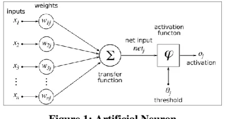
A typical artificial neuron and the modeling of a multilayered neural network are illustrated in the signal flow
from inputs x1 , ..., xnis considered to be unidirectional, which are indicated by arrows, as is a neuron’s output
signal flow (O). The neuron output signal O is given by the following relationship.
…….. (1)
wherewj is the weight vector, and the function f(net) is referred to as an activation (transfer) function. The
variable net is defined as a scalar product of the weight and input vectors,
…..(2)
where T is the transpose of a matrix, and, in the simplest case, the output value O is computed as:
…(3)
where is called the threshold level; and this type of node is called a linear threshold unit. In different types of
neural networks, most commonly used is the feed-forward error back-propagation type neural nets. In these
networks, the individual elements neurons are organized into layers in such a way that output signals from the
neurons of a given layer are passed to all of the neurons of the next layer. Thus, the flow of neural activations
Figure 1: Artificial Neuron
3.2 Back Propagation Training Algorithms
MATLAB tool box is used for neural network implementation for functional approximation for demand
forecasting. Different back propagation algorithms in use in MATLAB ANN tool box are:
• Batch Gradient Descent (traingd)
• Variable Learning Rate (traingda, traingdx)
• Conjugate Gradient Algorithms (traincgf, traincgp, traincgb, trainscg)
• Levenberg-Marquardt (trainlm)
3.3 Levenberg-Marquardt Algorithm (trainlm)
Like the quasi-Newton methods, the Levenberg-Marquardt algorithm was designed to approach second-order
training speed without having to compute the Hessian matrix. When the performance function has the form of a
sum of squares (as is typical in training feed forward networks), then the Hessian matrix can be approximated
as:
H = J TJ ………..(4)
And the gradient can be computed as
G = J Te ………..(5)
where is J the Jacobian matrix that contains first derivatives of the network errors with respect to the weights
and biases, and e is a vector of network errors. The Jacobian matrix can be computed through a standard back
propagation technique that is much less complex than computing the Hessian matrix. The Levenberg-Marquardt
algorithm uses this approximation to the Hessian matrix in the following Newton like update.
X
(k+1)=X
k-
J
TJ +µI
-1J
Te ……....(6)
This algorithm appears to be the fastest method for training moderate-sized Fed forward neural networks (up to
several hundred weights). It also has a very efficient MATLAB implementation, since the solution of the matrix
equation is a built-in function, so its attributes become even more pronounced in a MATLAB setting.
IV. RESULTS
The monthly sales data of the distributor, between the years of 2011-2013, are used to train the networks as
inputs and outputs, and then the demand pattern forecasts for 12 months of 2014 are made based on time series
analysis. Matlab 7.0 is used for ANN simulation. We have a product data available from 2011 to 2013. The data
of fuel filter available from privious year 2011 to 2013 in above table, privious data alrady consumed in large
chain managment, now we will first all consider the base year data of 2011 in 12th month to calculate next year
data of 2012 but 2012 data are available but can not consider as a forecasting data only consider as a target data.
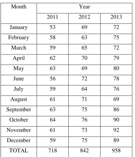
Table 1: Product Data of Fuel Filter for the Year 2011 to 2013
Month Year
2011 2012 2013
January 53 69 72
February 58 63 75
March 59 65 72
April 62 70 79
May 63 69 80
June 56 72 78
July 59 64 76
August 61 71 69
September 63 75 86
October 64 76 90
November 61 73 92
December 59 75 89
TOTAL 718 842 958
To calculate the forecasting error between actual data of 2012 and forecasting data 2013 and also formula
available for the calculating of forecasting error in MATLAB coding.
Forecasting r =abs(frcst-target’)and also calculate the percetage error using formula are pe=(forecasting
r/target)*100;
The data of fuel filter available from privious year 2011 to 2013 in above table, privious data alrady consumed
in large company, and month wise data consumptions are show in above table and find the next year data for the
supply chain managment, now we will first all consider the base year data of 2012 in 12th month to calculate
next year data of 2014 but 2013 data are available but can not consider as a forecasting data only consider as a
target data.
To calculate the forecasting error between actual data of 2012 and forecasting data 2013 and also formula
available for the calculating of forecasting error in MATLAB coding. forecasting r=abs(frcst-target’)and also
calculate the percetage error using formula are pe=(forecasting r/target)*100;
The data of fuel filter available from privious year 2011 to 2013 in above table, privious data alrady consumed
in large company, and month wise data consumptions are show in above table and find the next year data for the
supply chain managment, now we will first all consider the base year data of 2012 in 12th month to calculate
next year data of 2014 but 2013 data are available but can not consider as a forecasting data only consider as a
target data. To calculate the forecasting error between actual data of 2013 and forecasting data 2014 and also
formula vailable for the calculating of forecasting error in MATLAB coding forecasting r=abs(frcst-target’)and
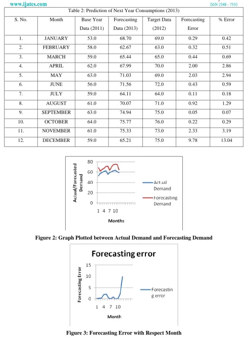
Table 2: Prediction of Next Year Consumptions (2013)
S. No. Month Base Year
Data (2011)
Forecasting
Data (2013)
Target Data
(2012)
Forecasting
Error
% Error
1. JANUARY 53.0 68.70 69.0 0.29 0.42
2. FEBRUARY 58.0 62.67 63.0 0.32 0.51
3. MARCH 59.0 65.44 65.0 0.44 0.69
4. APRIL 62.0 67.99 70.0 2.00 2.86
5. MAY 63.0 71.03 69.0 2.03 2.94
6. JUNE 56.0 71.56 72.0 0.43 0.59
7. JULY 59.0 64.11 64.0 0.11 0.18
8. AUGUST 61.0 70.07 71.0 0.92 1.29
9. SEPTEMBER 63.0 74.94 75.0 0.05 0.07
10. OCTOBER 64.0 75.77 76.0 0.22 0.29
11. NOVEMBER 61.0 75.33 73.0 2.33 3.19
12. DECEMBER 59.0 65.21 75.0 9.78 13.04
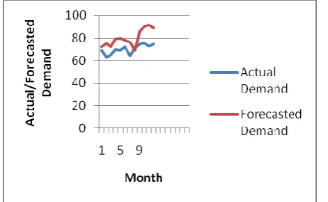
Figure 2: Graph Plotted between Actual Demand and Forecasting Demand
Figure 4: Graph Plotted Between Actual Demand and Forecasting Demand
V. CONCLUSION
In this project we have observed performance of product demand forecasting. The project is consumer product
for future average. The effectiveness of forecasting the demand signals in the supply chain with ANN method
and identify the best training method. This study has developed a cooperative forecastingmechanism based on
ANN and training methods. The proposed methodology, demand forecasting issue was investigated on a
manufacturing company as a real-world case study. The result indicates a TrainLM method performs more
effectively than the other tanning method and the more reliable forecast for our case. The proposed methodology
can be considered as a successful decision support tool in forecasting. The ability to increase forecasting
accuracy will result. Future research can possibility of using Artificial Neural Network to make a similar
approach and better the accuracy.
REFERENCES
[1]. Aburto L and Weber L (2007), “Improved Supply Chain Management Based on Hybrid Demand
Forecasts”, Applied Soft Computing, Vol. 7, pp. 136-144.
[2]. Anandhi V and ManickaChezian R (2012), “Backpropagation Algorithm for Forecasting the Price of
PulpwoodEucalyptus”, International Journal of Advanced Research in Computer Science, pp. 355-357.
[3]. Anandhi V, ManickaChezian R and Parthiban K T (2012), “Forecast of Demand and Supply of Pulpwood
Using Artificial Neural Network”, International Journal of Computer Science and Telecommunications,
pp. 35-38.
[4]. Carbonneau R, Laframboise K and Vahidov R (2008), “Application of Machine Learning Techniques for
Supply Chain Demand Forecasting”, European Journal of Operational Research, Vol. 184, pp. 1140-1154.
[5]. Chiu M and Lin G (2004), “Collaborative Supply Chain Planning Using the Artificial Neural Network
Approach”, Journal of Manufacturing Technology Management, Vol. 15, No. 8, pp. 787-796.
[6]. 6. Chopra S and Meindl P (2004), “Supply Chain Management: Strategy, Planning and Operation, Prentice
Hall.
[7]. Choy K L, Lee W B and Lo V (2003), “Design of an Intelligent Supplier Relationship Management
System: A Hybrid Case Based Neural Network Approach”, Expert Systems with Applications, in
[8]. Dejonckheere J, Disney S M, Lambrecht M R and Towill D R (2003), “Measuring and Avoiding the
Bullwhip Effect: A Controltheoretic Approach”, European Journal of Operational Research, Vol. 147, No.
3, pp. 567-590.
[9]. Gabriel Rilling, Patrick Flandrin and Paulo Goncalves (2009), “On Empirical Mode Decomposition and its
Algorithms”.
[10].Gabriel Rilling, Patrick Flandrin and Paulo Goncalves (2004), “Detrending and Denoising with Empirical
Mode Decompositions”.
[11].Gerson Lachtermacher and David Fuller J (2006), “Back Propagation in TimeSeries Forecasting”.
[12].Jeremy F Shapiro (2001), Modeling the Supply Chain, Wadsworth Group, A Division of Thomson
Learning, America.
[13].Kandananond K (2011), “Forecasting Electricity Demand in Thailand with an Artificial Neural Network
Approach”, Energies, Vol. 4, pp. 1246-1257.
[14].Karin Kandananond (2012), “Consumer Product Demand Forecasting Based on Artificial Neural Network
and Support Vector Machine”, World Academy of Science, Engineering and Technology, Vol. 63, pp.
372-375.
[15].Ralf Herbrich, Max Keilbach, ThoreGraepel, Peter Bollmann–Sdorra and Klaus Obermayer (1999),
“Neural Networks in Economics: Background, Applications and New Developments”, Advances in
Computational Economics: Computational Techniques for Modeling Learning in Economics, Vol. 11, pp.
169-196.
[16].Norden E Huang, Zheng Shen, Steven R Long, Manli C Wu, Hsing H Shih, Quanan Zheng, Nai-Chyuan
Yen, Chi Chao Tung and Henry H Liu (1998), “The Empirical Mode Decomposition and the
HilbertSpectrum for Nonlinear and NonStationary Time Series Analysis”, Vol. 454, No. 1971.
[17].Shapiro J F (2001), Modeling the Supply Chain, Duxbury Thomson Learning Inc., CA.
[18].Simon Haykin (2001), “Kalman Filtering and Neural Networks”, John Wiley & Sons Inc., ISBNs:
0-471-36998-5 (Hardback), 0-471-22154-6 (Electronic).
[19].Tsiakis P, Shah N and Pantelides C C (2001), “Design of Multi-Echelon Supply Chain Networks Under
Demand Uncertainty”, Ind. Eng. Chem. Res., Vol. 40, pp. 3585-3604.
[20].Yanxiang He, Feng Li, Zhikai Song and Ge Zhang (2002), “Neural Networks Technology for Inventory