Determination of optical and microphysical properties of thin warm clouds using ground based hyper-spectral analysis

Atmos. Meas. Tech., 5, 851–871, 2012 www.atmos-meas-tech.net/5/851/2012/ doi:10.5194/amt-5-851-2012

© Author(s) 2012. CC Attribution 3.0 License.

Atmospheric

Measurement

Techniques

Determination of optical and microphysical properties of thin warm

clouds using ground based hyper-spectral analysis

E. Hirsch1, E. Agassi2, and I. Koren1

1_{Department of Environmental Sciences, Weizmann Institute, Rehovot, 76100, Israel}

2_{Department of Environmental Physics, Israel Institute for Biological Research, Nes-Ziona, 74100, Israel}

Correspondence to: E. Hirsch ([email protected])

Received: 2 November 2011 – Published in Atmos. Meas. Tech. Discuss.: 12 December 2011 Revised: 13 March 2012 – Accepted: 12 April 2012 – Published: 27 April 2012

Abstract. Clouds play a critical role in the Earth’s radiative budget as they modulate the atmosphere by reflecting short-wave solar radiation and absorbing long short-wave IR radiation emitted by the Earth’s surface. Although extensively studied for decades, cloud modelling in global circulation models is far from adequate, mostly due to insufficient spatial resolu-tion of the circularesolu-tion models. In addiresolu-tion, measurements of cloud properties still need improvement, since the vast ma-jority of remote sensing techniques are focused in relatively large, thick clouds. In this study, we utilize ground based hy-perspectral measurements and analysis to explore very thin water clouds. These clouds are characterized by liquid wa-ter path (LWP) that spans from as high as∼50g m−2 and down to 65 mg m−2 _{with a minimum of about 0.01 visible} optical depth. The retrieval methodology relies on three ele-ments: a detailed radiative transfer calculations in the long-wave IR regime, signal enhancement by subtraction of a clear sky reference, and spectral matching method which exploits fine spectral differences between water droplets of different radii. A detailed description of the theoretical basis for the retrieval technique is provided along with a comprehensive discussion regarding its limitations. The proposed method-ology was validated in a controlled experiment where artifi-cial clouds were sprayed and their effective radii were both measured and retrieved simultaneously. This methodology can be used in several ways: (1) the frequency and optical properties of very thin water clouds can be studied more pre-cisely in order to evaluate their total radiative forcing on the Earth’s radiation budget. (2) The unique optical properties of the inter-region between clouds (clouds’ “twilight zone”) can be studied in order to more rigorously understanding of the governing physical processes which dominate this region.

(3) Since the optical thickness of a developed cloud gradually decreases towards its edges, the proposed methodology can be used to study the spatial microphysical behaviour of these edges. (4) A spatial-temporal analysis can be used to study mixing processes in clouds’ entrainment zone.

1 Introduction

Clouds play a critical role in the Earth’s radiative budget as they modulate the atmosphere by reflecting shortwave solar radiation and absorbing longwave IR (LWIR) radiation emit-ted by the Earth’s surface (Ramanathan et al., 1989). The ra-diative forcing of a single cloud depends on its height, thick-ness, and optical properties (Trenberth et al., 2009), and their accumulated effect depends on their lifetime, global cover-age, and frequency of occurrence (Wylie et al., 2005). Shal-low clouds are usually considered to have a net negative ra-diative forcing (cooling effect) as they reflect a substantial amount of the received solar irradiance while they have a mi-nor effect on the total thermal radiation emitted by the Earth, since the magnitude of their emitted radiation is comparable with a cloud free surface. On the other hand, high clouds, such as anvils (Koren et al., 2010) or cirrus, might have a positive radiative forcing, since they have a relatively low reflectance in the visible portion of the spectrum, while the thermal contrast between them and the Earth is large. The effect of clouds on the Earth’s radiative budget is so pro-found, that it has been shown that an increase of 15–20 % in the amount of low clouds could balance the expected heating effect of doubling the CO2concentration in the atmosphere (Slingo, 1990).

852 E. Hirsch et al.: Determination of optical and microphysical properties of thin warm clouds Although extensively studied for decades, cloud modelling

in global circulation models (GCM) is far from adequate (Tselioudis and Jakob, 2002), mostly due to insufficient spa-tial resolution of the circulation models, which results in poor representation of the small scale microphysical processes that control clouds’ properties (Heintzenberg and Charlson, 2009). Furthermore, cloud sensing techniques also need im-provement (Turner et al., 2007), since most of the techniques which have been developed are oriented to relatively thick clouds that can be easily observed from space-borne plat-forms. Over the years, numerous algorithms have been sug-gested to retrieve clouds’ properties by remote sensing mea-surements. These algorithms exploit radiative information in wavelengths from nanometeres to millimeters and can be characterized by the observation point – space or ground based measurements, and by the sensing method – either ac-tive or passive.

Although different approaches have been proposed, all of these methods are similar to some extent: they depend upon radiative (e.g. optical thickness and albedo) and microphysi-cal (e.g. droplet size distribution and thermodynamic phase) properties of the clouds. The theoretical basis for determin-ing the optical thickness and effective radius of clouds by us-ing reflected solar radiation was introduced by Nakajima and King (1990). Later, the Special Sensor Microwave/Imager (SSM/I) was used to retrieve liquid water content of clouds over the ocean (Weng and Grody, 1994). In addition, it was suggested that clouds liquid water and temperature could be derived by using an array of ground based devices, namely, microwave radiometer, ceilometer, radio acoustic sounding system and various surface meteorological instruments (Han and Westwater, 1995). The utility of space-borne multispec-tral passive remote sensing for retrieval of optical and mi-crophysical properties for numerous cloud types was demon-strated (King et al., 1997). On the other hand, ground based cloud radars were used to retrieve the droplets effective ra-dius profile of stratus clouds, by analyzing the radar reflec-tivity under various assumptions regarding the total number of droplets in the clouds (Frisch et al., 2002). More recently, the passive MODIS Airborne Simulator (MAS) was used to extract cloud properties even over snow and icy backgrounds (King et al., 2004). A noteworthy method to retrieve thin cloud’s properties was presented by Turner (2005), who uti-lized ground based IR high spectral resolution measurements to retrieve mixed-phase cloud properties. The method suc-cessfully obtained the properties of simulated and measured thin water clouds with visible optical depths in the range of 0.2–4. The retrieval is based on an optimal estimation ap-proach to fit a measured spectrum to a spectral database that was created by a radiation transfer model. This spectral anal-ysis paradigm, is widely used in retrieval algorithms which exploit multispectral analysis.

As stated above, the main interest of the majority of the remote sensing techniques are relatively large, opti-cally thick clouds, which contribute substantially to the total

clouds forcing and to the Earth’s albedo. However, Turner et al. (2007) have overviewed the importance of thin liquid wa-ter clouds and the challenge in correctly retrieving their prop-erties. In their work, they have defined thin clouds as clouds with liquid water path (LWP) up to 100 g m−2and have com-pared the performance of almost 20 different algorithms in retrieving the properties of a single layer, overcast, stratocu-mulus cloud field. The remote sensing techniques considered were wide ranging and spanned from the visible to the mi-crowave portion of the spectrum; from ground based to space borne; both passive and active. The authors’ main conclusion was that huge discrepancies exist among the different algo-rithms (even among algoalgo-rithms that are in the same general classification), and that the cloud properties retrieval commu-nity should examine the accuracy of the algorithms when thin clouds are considered. An additional complexity to the chal-lenges in correctly retrieving thin clouds properties arises from their expected occurrences. Koren et al. (2008) have studied the dependence of clouds’ frequency (in a sparse cu-mulus cloud field) on their apparent size and showed that a power law governs the connection. This means that the num-ber of clouds with a given area is proportional to the inverse of am, where a is the cloud area and m is the power ex-ponent of the distribution (1< m <2). They concluded that the smallest detectable clouds may contribute significantly to the total cloud area as well as for the mean cloud field reflectance. This analysis coincides well with studies (Ko-ren et al., 2007) which identified optically unique properties of the clouds’ inter region (also known as “the clouds’ twi-light zone”). This region is characterized by a decrease in the apparent optical depth as the distance from the nearest de-tectable cloud increases. The precise nature of the “twilight zone” is still unclear, although several mechanisms have been suggested to explain its optical properties: undetected cloud fragments, aerosol humidification, and nearby scattering of solar radiation by clouds, are only some of the main sug-gested explanations. As most of the current retrieval meth-ods are applied to space borne sensor data, thin warm clouds are usually ignored due to insufficient spatial and temporal resolution. In particular, the transition zone between clouds and clear skies is usually classified into one of two possible states: cloudy or clear. In spite of the knowledge gaps regard-ing the nature of thin, warm clouds, the relationship between their LWP and effective radius was studied. Liu et al. (2003) found high correlation between clouds’ LWP and their effec-tive radius: thin, undeveloped clouds, which contain small amounts of LWP, are characterized by small effective radii as well. In fact, Liu et al. (2003) showed that the majority of clouds with LWP smaller than 25 g m−2had effective ra-dius smaller than 5 µm. Luckily (and as presented later in this manuscript), our proposed method is at its highest quan-titative sensitivity for clouds with small effective radii. The purpose of our study is to introduce a new concept to deter-mine and retrieve the effective radius, LWP, and optical depth of very thin warm clouds by using ground based IR spectral

E. Hirsch et al.: Determination of optical and microphysical properties of thin warm clouds 853 measurements. These kinds of measurements and analysis

might shed light on some of the most interesting enigmas of cloud microphysics and interaction with aerosols, and the clouds’ effect on the radiative budget of the Earth.

In this study, we will utilize ground based infrared spec-tral analysis and measurements in order to explore very thin water clouds which are characterized by liquid water path that varies from as high as 50 g m−2and down to 65 mg m−2 with a minimum of approximately 0.01 visible optical depth. The following section will introduce the theoretical basis for ground based passive sensing of the thermal IR spectrum of the zenith sky. The retrievals for the cloud effective radius and liquid water path (and the optical depth as a result) will be developed. The spectral differences in the extinction ef-ficiencies of water droplets with different radii will be ex-amined and the effect of these differences on the radiative transfer calculations will be discussed. We will show that thin liquid water clouds which contain varying liquid water paths and effective radii alter the magnitude and the spec-trum of the downwelling IR sky radiation. We will demon-strate how adequate spectral analysis can serve as a trigger for a mathematical best fit retrieval algorithm. This concept results in a standalone algorithm which first spectrally iden-tifies the physical phenomenon which formed the measured signal, and only then is the optimal solution chosen in terms of mathematical best fit. The limitations of the method are discussed in Sect. 3 by an overview of the methodology’s sensitivity to fluctuations in the relative humidity field, at-mospheric aerosols, and haze. Section 4 describes the ex-perimental setup used to validate the proposed methodology, while Sect. 5 presents a case study of a natural cloud that was measured during a field campaign. The main conclu-sions of these results and future work are discussed in detail in Sect. 6.

2 The downwelling radiance of the zenith sky in the presence of thin warm clouds in the long wave IR spectral band

In this section we will explore the theoretical basis for the spectral variability of the zenith sky radiance in the LWIR, in the presence of thin warm clouds. We will show that clouds which differ by their effective droplets radii alter the down-welling sky radiance in a manner that can be identified by high spectral resolution measurements. Nevertheless, these spectral differences are small when compared to the clear sky background, and therefore a differential analysis tech-nique is required in order to extract them from the clear sky background signature. As will be presented, this technique exploits the advantages of ground based, high temporal reso-lution measurements.

We will first explore how the obtained spectral properties of a single water droplet varies with its radius. Then a brief introduction to the analytical methods which have been used

33

1

Figure 1 - Extinction efficiency Vs. wavelength for water droplets at different radii. Note the

2

evident spectral difference of the various droplets. This analysis suggests that thin water

3

clouds which differ by their droplet's effective radius, might have a unique spectrum in the

4

LWIR. As a result, it might be possible to discriminate between water droplets of different

5

sizes.

6

7

Figure 2 - An example of the SAM (Spectral Angle Mapping) index of two spectra. SAM

8

considers a measured spectrum in n wavelengths (n=3 in this example) as a vector in an n

9

dimensional space (B

, B

, B

). The spectral similarity between a measured spectrum (V) and

10

a reference spectrum (V

) is simply the angle α between these two spectra, calculated to be

11

)

(

cos

ref ref

v

v

v

v

















. Distinct spectra will produce relatively large SAM values, while similar

12

spectra will produce small values.

13

14

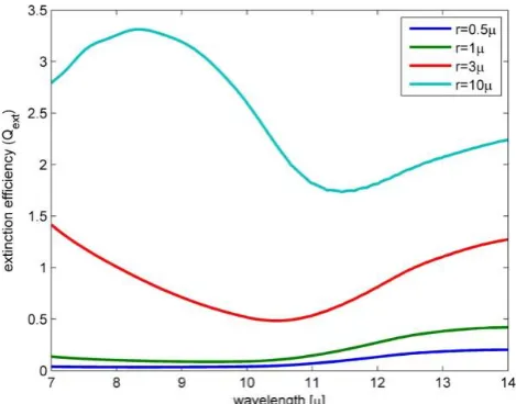
Fig. 1. Extinction efficiency vs. wavelength for water droplets at different radii. Note the evident spectral difference of the various droplets. This analysis suggests that thin water clouds which differ by their droplet’s effective radius, might have a unique spectrum in the LWIR. As a result, it might be possible to discriminate between water droplets of different sizes.

in this study is provided. Following that, we analyze the ef-fect of thin monodisperse and polydisperse water clouds on the measured sky LWIR radiance. Finally, at the end of this section, we provide a detailed scheme of a retrieval method for the microphysical and the optical properties of very thin water clouds. This method is based on a spectral comparison between measured spectra and a spectral library created by radiative transfer calculations.

2.1 The spectral dependence of the extinction efficiency on the droplet’s radius

The presence of water droplets in the atmosphere affects the magnitude and the spectrum of the LWIR sky radiation that reach the surface. The interaction of the radiation with the droplets is described by the generalized Mie (1908) the-ory, which derives a wave equation with boundary condi-tions at the surface of a sphere by solving Maxwell’s equa-tions. The extinction, absorption, and scattering efficiencies are commonly characterized as a function of the size param-eter (which is defined asx= 2π r/λ, whereris the droplet’s radius andλis the radiation wavelength). An alternative way to characterize the interaction of radiation and water droplets is to examine the mentioned efficiencies in a certain spec-tral region (e.g. the LWIR), for different droplets’ radii. Such analysis reveals variations in the extinction efficiencies of droplets with different radii (Fig. 1). The refractive index of water (Palik, 1997), was used in order to calculate the extinc-tion, absorpextinc-tion, and scattering efficiencies (M¨atzler, 2002). The scattering coefficient is larger than the absorption coef-ficient (per unit length), therefore scattering is the dominant

854 E. Hirsch et al.: Determination of optical and microphysical properties of thin warm clouds mechanism in which water attenuates the impinging LWIR

radiation. Apart from the evident differences in the magni-tude of the extinction efficiency, one can notice how the ex-tinction spectrum depends on the droplets radii. These spec-tral variations suggest that thin warm clouds with different droplets’ effective radii might modify the down-welling sky radiance in distinct spectral forms. In the following subsec-tions we will examine the latter hypothesis, by using a ra-diative transfer model which incorporates the optical prop-erties of water clouds containing different water droplet size distributions.

2.2 Analysis methodology

The attempt to extract physical properties of remotely sensed objects is commonly referred to as solving an inverse prob-lem. A typical approach to apply it is composed of a forward model that predicts the expected signal under certain atmo-spheric parameters, and a mathematical curve fitting tech-nique and threshold criteria to decide which atmospheric pa-rameters present the most probable solution (Rodgers, 2000). As detailed hereafter, the presented methodology follows this general approach but with important modification prior to the stage of curve fitting technique. The presented approach treats thin warm clouds as semi transparent objects which al-ter the magnitude and the spectrum of the clear background signal. Therefore, we have used techniques borrowed from the field of remote detection and identification of gaseous and aerosols plumes for environmental applications, under the assumption that they are the most suitable tools to re-trieve thin clouds’ properties (see for example, Hirsch and Agassi, 2007, and Agassi et al., 2008).

The analysis presented in this study relies on 3 elements: a radiation transfer model, a method to extract the effect of a water cloud while eliminating the sky background, and a spectral matching method. A brief overview of each element is given in the following subsections.

2.2.1 Radiative transfer model

In this study, the PCModWin4.0 software, which includes the MODTRAN model (Berk et al., 1989), was used to predict the expected zenith sky radiance in the presence of various thin water clouds. MODTRAN is a radiation transfer model developed by the US Air Force Research Laboratory. It is based on the HITRAN2000 database (Rothman et al., 2003) and it solves the radiative transfer equation including the ef-fects of molecular and particulate absorption/emission and scattering, surface reflections and emission, solar/lunar illu-mination, and spherical refraction. The atmosphere is mod-eled as plane parallel (horizontally homogeneous), and its constituent profiles, both molecular and particulate, may be defined by using built-in models or by user-specified vertical profiles. The spectral range extends from the UV into the far-infrared and the user can define up to 4 aerosol types with

distinct optical properties and incorporate each aerosol in the atmospheric column with specific extinction, absorption, and scattering coefficients. In our analysis, the MODTRAN input included the sounded atmospheric profile, the vertical extent of the cloud, and its water droplets’ optical properties which were calculated for every simulated cloud.

2.2.2 Signal enhancement by sky background elimination

The presence of a thin water cloud alters the clear sky IR radiation. Unfortunately, as demonstrated in Sect. 2.3 be-low, the magnitude of the signal contributed only by the thin cloud is very small compared to the signal emerging from the clear sky itself. Therefore, in order to enhance the cloud’s signature, we subtract the clear sky signal from the obtained spectra. The method of clear reference subtraction is commonly applied for detection and identification of weak gaseous plumes (Hirsch and Agassi, 2007). It enables re-trieval of only the differential spectral signal, and therefore analyzes the phenomenon which created the signal without considering the background. This method is particularly ad-vantageous for weak semi-transparent objects that otherwise could not be analyzed, and in the following we will show how apparent similar spectra become spectrally distinctive when the clear sky reference is removed.

2.2.3 Spectral analysis

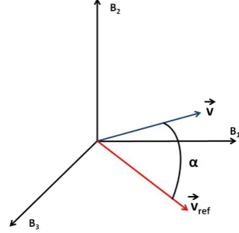
The process of subtracting the clear sky reference creates a differential spectrum. In order to classify the phenomenon which caused the differential signal, we assess its spectral similarity with a predicted set of library spectra which was pre-calculated. As commonly applied for identification of known reference spectra (Yuhas et al., 1992; Park et al., 2007), we have utilized the SAM – Spectral Angle Mapping (Kruse et al., 1993) analysis on the differential spectral signa-tures (Fig. 2). The SAM considers the spectral signals (each consisting ofn wavelengths) as vectors in an-dimensional space, and calculates the angle between two spectra as a mea-sure of their similarity. The angle between two spectra can be any value between 0◦ (perfect match), through 90◦ (or-thogonal spectra), to 180◦(two spectra pointing to opposite directions). Namely, distinct spectra will produce relatively large SAM values, while similar spectra will produce small values. As in any remote sensing retrieval, a certain threshold must be applied, and its value depends on the application and should be determined empirically. In the proposed method, and as described later, we have applied a SAM threshold of 10◦. The SAM metric is especially efficient when small spectral features are present, even though the complete spec-tral behaviour appears similar. Throughout this study, the SAM method has been applied on spectra which contained 16 wavelengths in the region of 8–9 µm and 51 wavelengths in the region of 10–13 µm. These wavelengths were chosen to

E. Hirsch et al.: Determination of optical and microphysical properties of thin warm clouds 855

33 1

Figure 1 - Extinction efficiency Vs. wavelength for water droplets at different radii. Note the

evident spectral difference of the various droplets. This analysis suggests that thin water

clouds which differ by their droplet's effective radius, might have a unique spectrum in the

LWIR. As a result, it might be possible to discriminate between water droplets of different

sizes.

7

Figure 2 - An example of the SAM (Spectral Angle Mapping) index of two spectra. SAM

considers a measured spectrum in n wavelengths (n=3 in this example) as a vector in an n

dimensional space (B

, B

, B

). The spectral similarity between a measured spectrum (V) and

a reference spectrum (V

) is simply the angle α between these two spectra, calculated to be

)

(

cos

ref ref

v

v

v

v

















. Distinct spectra will produce relatively large SAM values, while similar

12

spectra will produce small values.

14

Fig. 2. An example of the SAM (Spectral Angle Mapping) index of two spectra. SAM considers a measured spectrum inn wave-lengths (n= 3 in this example) as a vector in anndimensional space (B1,B2,B3). The spectral similarity between a measured spectrum (V) and a reference spectrum (Vref) is simply the angleαbetween these two spectra, calculated to beα= cos−1 v vref

||v|| · ||vref||

. Dis-tinct spectra will produce relatively large SAM values, while similar spectra will produce small values.

match with the spectro-radiometer features used in our mea-surements (Sect. 4). The spectral region of 9–10 µm was de-liberately omitted since it contains the wide ozone absorption line (McCaa and Shaw, 1968), that might induce errors in the analysis.

2.3 The LWIR sky radiance in the presence of very thin warm monodisperse and polydisperse clouds In this subsection we will investigate the spectral effect of very thin water clouds on the down welling IR radiance of the clear sky. Throughout this study we will use the atmospheric profile measured with a radiosonde in the Beit-Dagan station (http://weather.uwyo.edu/upperair/sounding.html), on 8 Au-gust 2010, 12:00 UTC (Fig. 3), as an input for the radiative transfer calculations. During the Israeli summer, there is a steady downwelling warm air settling over the Middle East that originates from the tropics. Therefore, a strong inversion layer is present, and only very shallow clouds can form. The occurrence of precipitation is almost impossible. In addition, the all area is dominated by steady westerly winds which arise from a constant low pressure over the Persian Gulf. This low pressure itself is a branch of the Indian summer monsoon. Since the Israeli summer is characterized by inac-tive weather and very stable meteorological conditions, the chosen atmospheric profile represents a typical Israeli day-time summer profile. According to the ceilometer readings in the Ben-Gurion airport (http://weather.uwyo.edu/surface/ meteogram/), which is located approximately 10 km from our measurement site, the average cloud base height was

34

1

Figure 3 - Atmospheric profile (relative humidity in red, and air temperature in black) on 8

2

August 2010, 12:00UTC (Website: “Atmospheric Sounding”). The shallow inversion layer is

3

noticeable at a height of about 600m.

4

5

6

Figure 4 – The expected spectral signature of the zenith sky in the presence of 50 meter thick

7

monodisperse clouds with liquid water content of 15mg/m

at 800m above the ground. Every

8

cloud is characterized by different water droplets radii. At first glance, the spectral signatures

9

appear extremely similar.

10

Fig. 3. Atmospheric profile (relative humidity in red, and air tem-perature in black) on 8 August 2010, 12:00 UTC (http://weather. uwyo.edu/upperair/sounding.html). The shallow inversion layer is noticeable at a height of about 600 m.

792 m during the morning hours. Therefore, all the radia-tive transfer calculations simulated clouds at 800 m above the surface.

2.3.1 The effect of monodisperse water clouds on the LWIR sky radiance

The extinction coefficient per unit length of a monodisperse water cloud with a given liquid water content (LWC) is given by

σext(λ) = N π r2Qext(λ, r) (1) whereris the droplet radius, andQext(λ, r)is the extinction efficiency of a single water droplet with radiusr at wave-lengthλ. N is the droplet density (i.e. the number of droplets per unit volume) which equals the LWC divided by the mass of a droplet, i.e.N= LWC/(4/3π r3 ρ) (whereρis the den-sity of water, taken here in mks units as 1000 kg m−3). Ex-actly the same formulation holds for deriving the absorption and scattering coefficients (σabs(λ)andσsct(λ), respectively) per unit length. These spectral coefficients are used to solve the radiative transfer equations in the presence of clouds.

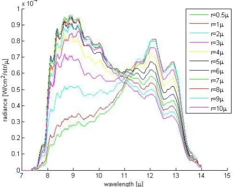
A set of 50 m thick, monodisperse clouds with equal liquid water content of 15 mg m−3, were simulated at equal heights and under the same atmospheric profile. The only difference between the clouds was the water droplet radius. The ex-pected zenith sky LWIR radiances in the presence of the simulated clouds are presented (Fig. 4). The figure creates an impression that the anticipated spectra are quite similar, since most of the signal originates from the clear sky back-ground. As explained above, subtraction of the clear refer-ence eliminates the sky background and extracts the sole ef-fect of the thin clouds (Fig. 5). The differential spectra appear quite distinct as small droplets attenuate more radiation in the

856 E. Hirsch et al.: Determination of optical and microphysical properties of thin warm clouds

34

1

Figure 3 - Atmospheric profile (relative humidity in red, and air temperature in black) on 8

2

August 2010, 12:00UTC (Website: “Atmospheric Sounding”). The shallow inversion layer is

3

noticeable at a height of about 600m.

4

5

6

Figure 4 – The expected spectral signature of the zenith sky in the presence of 50 meter thick

7

monodisperse clouds with liquid water content of 15mg/m

at 800m above the ground. Every

8

cloud is characterized by different water droplets radii. At first glance, the spectral signatures

9

appear extremely similar.

10

Fig. 4. The expected spectral signature of the zenith sky in the pres-ence of 50 m thick monodisperse clouds with liquid water content of 15 mg m−3at 800 m above the ground. Every cloud is charac-terized by different water droplets radii. At first glance, the spectral signatures appear extremely similar.

11–13 µm region while large droplets attenuate more radia-tion in the 8–9 µm region. The use of the SAM index on the differential spectra (Fig. 6) quantifies the apparent spectral variations of the sky radiance in the presence of thin clouds. Three distinctive areas appear in the mutual cross SAM ma-trix of the differential spectra: (1) small water droplets with radii less than 2 µm have spectral signals which are rela-tively similar (low cross SAM values), while their spectra are distinct from water droplets with higher radii. (2) Medium size water droplets with radii of 2–3 µm are different from water droplets with other radii. (3) Spectra of larger water droplets with radii greater than 4 µm appear spectrally differ-ent than smaller droplets, but the ability of the technique to distinguish between droplets in the region of 4–10 µm is rel-atively low. These distinctive areas reinforce the hypothesis that spectral variations in the extinction efficiencies alter the radiation in a spectrally different manner, and that using the SAM on the differential spectral signatures might be useful to distinguish between clouds with different droplets’ effec-tive radii.

2.3.2 The effect of polydisperse water clouds on the LWIR zenith sky radiance

Clouds droplets are not monodisperse. The size distribution of water droplets of cumulus clouds has been extensively studied for several decades. A modified Gamma function was proposed to represent the density size distribution of clouds’ droplets as a function of their radius (Deirmendjian, 1964). Specifically, the size distribution is given by

n(r) = a rαe−brγ (2)

35

1

Figure 5 – The differential spectral signature of the various clouds presented in Figure 4.

2

Every signature in this figure is the result of subtracting the clear sky signature (see Figure 4)

3

from the expected sky radiance in the presence of a cloud. One can notice the evident spectral

4

difference caused by different water droplets` radii. Clouds with small water droplets

5

attenuate more radiation in the 11µm-13µm, while clouds with larger droplets affect more in

6

the 8µm-9µm.

7

8

9

Figure 6 – Cross SAM values of the differential spectral signatures formed by thin clouds

10

(Figure 5). Small values indicate the signatures are spectrally similar, while large values

11

indicate the signatures are spectrally distinct. Three distinctive areas exist in the matrix: 1)

12

small water droplets with radii less than 2µm create spectral signatures which are relatively

13

similar (low cross SAM values), while their spectral signature is distinctive from water

14

droplets with higher radii. 2) Medium water droplets with radii of 2µm-3µm are unique from

15

Fig. 5. The differential spectral signature of the various clouds pre-sented in Fig. 4. Every signature in this figure is the result of sub-tracting the clear sky signature (see Fig. 4) from the expected sky radiance in the presence of a cloud. One can notice the evident spectral difference caused by different water droplets‘ radii. Clouds with small water droplets attenuate more radiation in the 11–13 µm, while clouds with larger droplets affect more in the 8–9 µm.

wheren(r) is the normalized size distribution, i.e. ∞ R

0

n(r)

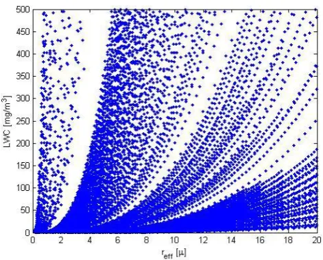
dr= 1, and a,α, b, and γ are positive constants. Utilizing the modified Gamma size distribution, we have created a large dataset of more than 120 000 size distributions of water droplets in order to cover a wide range of possible cases. The droplets size distributions which were used in our simulation (Table 1), represent typical distributions that were measured in natural low clouds (Miles et al., 2000). These simulated distributions span a 2-D space of effective radius (reff) and LWC (Fig. 7), which will later be used by MODTRAN to construct a spectral library of possible sky radiances in the presence of different water clouds. The effective radius is a commonly used parameter to represent the water droplets size distribution (Hansen and Travis, 1974). Specifically,

reff = ∞ R

0

r3n(r)dr

∞ R

0

r2_n(r)dr

(3)

and it is related to the visible optical depth of the cloud (Stephens, 1994), by

ODvis =

3 LWP 2ρ reff

(4) where LWP is the liquid water path in the cloud, namely LWP =

htop R

hbase

LWC(h)dh.

E. Hirsch et al.: Determination of optical and microphysical properties of thin warm clouds 857

Table 1. Parameters of clouds droplet size distributions used in our simulation (right column), and as summarized from vast in-situ measure-ments of droplets size distributions in low-level continental and marine Stratiform clouds (Miles et al., 2000). Values in parenthesis represent the parameter’s standard deviation

Parameter In-situ measurements Simulated

(Miles et al., 2000) droplets size

Continental Marine distributions

Mean radius[µm] 4.1 (1.95) 7.1 (1.7) 6.3 (3.8) Standard deviation above mean radius[µm] 1.55 (0.6) 2.9 (1) 3.4 (2.7) Effective radius[µm] 5.4 (2.05) 9.6 (2.35) 9.6 (6.5)

LWC[mg m−3] 190 (210) 180 (140) 118 (128)

35

1

Figure 5 – The differential spectral signature of the various clouds presented in Figure 4.

2

Every signature in this figure is the result of subtracting the clear sky signature (see Figure 4)

3

from the expected sky radiance in the presence of a cloud. One can notice the evident spectral

4

difference caused by different water droplets` radii. Clouds with small water droplets

5

attenuate more radiation in the 11µm-13µm, while clouds with larger droplets affect more in

6

the 8µm-9µm.

7

8

9

Figure 6 – Cross SAM values of the differential spectral signatures formed by thin clouds

10

(Figure 5). Small values indicate the signatures are spectrally similar, while large values

11

indicate the signatures are spectrally distinct. Three distinctive areas exist in the matrix: 1)

12

small water droplets with radii less than 2µm create spectral signatures which are relatively

13

similar (low cross SAM values), while their spectral signature is distinctive from water

14

droplets with higher radii. 2) Medium water droplets with radii of 2µm-3µm are unique from

15

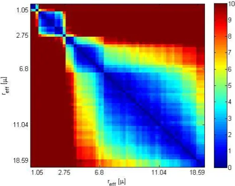
Fig. 6. Cross SAM values of the differential spectral signatures formed by thin clouds (Fig. 5). Small values indicate the tures are spectrally similar, while large values indicate the signa-tures are spectrally distinct. Three distinctive areas exist in the ma-trix: (1) small water droplets with radii less than 2 µm create spec-tral signatures which are relatively similar (low cross SAM values), while their spectral signature is distinctive from water droplets with higher radii. (2) Medium water droplets with radii of 2–3 µm are unique from water droplets with other radii. (3) Spectral signatures of larger water droplets with radii higher than 4 µm appear spec-trally different than smaller droplets, but the method’s capability to distinguish between droplets in the region of 4–10 µm is relatively low.

It is worth noticing that the use ofreffas a measure for the cloud optical depth is not valid in the IR region, as the orig-inal calculation ofreff (Hansen and Travis, 1974), assumed the droplet radius is noticeably larger than the wavelength, which is valid only in the visible portion of the spectrum. Nevertheless, in order to follow conventional characteriza-tion of clouds in the scientific community, we will use the

reffand ODvis parameters to characterize the simulated and measured clouds.

36

water droplets with other radii. 3) Spectral signatures of larger water droplets with radii higher

1

than 4µm appear spectrally different than smaller droplets, but the method's capability to

2

distinguish between droplets in the region of 4µm-10µm is relatively low.

3

4

5

Figure 7 - The space of LWC and effective radius of the different clouds that were used in this

6

analysis. Every point in this graph represents a modified Gamma size distribution with

7

distinct parameters. The size distribution is used to calculate the extinction, absorption, and

8

scattering coefficients for unit length of the simulated cloud.

9

10

11

Figure 8 - Cross SAM values of the differential spectral signatures of water clouds with

12

different effective radii with approximately constant LWC (14.5mg/m

<LWC<15mg/m

).

13

This figure shows that the spectral variability depends on the effective radius of the cloud:

14

Clouds with small r

(less than 1µm) are spectrally distinct, as their cross SAM values with

15

Fig. 7. The space of LWC and effective radius of the different clouds that were used in this analysis. Every point in this graph represents a modified Gamma size distribution with distinct parameters. The size distribution is used to calculate the extinction, absorption, and scattering coefficients for unit length of the simulated cloud.

In a similar manner to Eq. (1), the spectral extinction coef-ficient of a water cloud with a given droplet size distribution is

σext(λ) = N ∞ Z

0

n(r) π r2Qext(λ, r)dr (5)

whereN is the total number of water droplets per unit vol-ume, and n(r) is a normalized size distribution as defined previously.

The same cross SAM analysis on the differential spectral signatures of polydisperse water clouds (Fig. 8) shows that the spectral variability still holds even when the droplets fol-low a modified Gamma distribution function. From the fig-ure, it is obvious that clouds with smallreff (less than 1 µm) are spectrally distinct, as their cross SAM values with other clouds are relatively high. In the same manner, clouds with medium effective radius (1 µm< reff<2.75 µm) are easily

858 E. Hirsch et al.: Determination of optical and microphysical properties of thin warm clouds

36

water droplets with other radii. 3) Spectral signatures of larger water droplets with radii higher

1

than 4µm appear spectrally different than smaller droplets, but the method's capability to

2

distinguish between droplets in the region of 4µm-10µm is relatively low.

3

4

5

Figure 7 - The space of LWC and effective radius of the different clouds that were used in this

6

analysis. Every point in this graph represents a modified Gamma size distribution with

7

distinct parameters. The size distribution is used to calculate the extinction, absorption, and

8

scattering coefficients for unit length of the simulated cloud.

9

10

11

Figure 8 - Cross SAM values of the differential spectral signatures of water clouds with

12

different effective radii with approximately constant LWC (14.5mg/m

<LWC<15mg/m

).

13

This figure shows that the spectral variability depends on the effective radius of the cloud:

14

Clouds with small r

(less than 1µm) are spectrally distinct, as their cross SAM values with

15

Fig. 8. Cross SAM values of the differential spectral signatures of water clouds with different effective radii with approximately con-stant LWC (14.5 mg m−3<LWC<15mg m−3). This figure shows that the spectral variability depends on the effective radius of the cloud: Clouds with smallreff(less than 1 µm) are spectrally distinct, as their cross SAM values with other clouds are relatively high. Clouds with medium effective radius (1 µm< r_eff<2.75 µm) are easily distinguished by the SAM analysis. Clouds withreff>3 µm appear relatively similar to each other, but quite different from a cloud with smallerreff.

distinguished by the SAM analysis. Clouds withreff>3 µm appear relatively similar to each other, but quite different from clouds with smallerreff.

2.4 Retrieval methodology

Following the theoretical basis presented in the previous sub-sections, we propose the following methodology (Fig. 9), which is composed of 3 elements, for the retrieval of very thin liquid water clouds’ microphysical and optical properties:

a. Simulating the expected IR spectral signature of the zenith sky in the presence of very thin liquid wa-ter clouds with various microphysical and geometrical properties, namely effective radius, LWC, and geomet-rical depth. The usage of these three parameters allows us to refer to the simulated and retrieved clouds by four variables: effective radius, LWC, LWP, and optical depth, and we will use them interchangeably through-out this manuscript according to the scientific relevance. The simulation should use a radiative transfer model, that considers effects of molecular and particulate emis-sion and scattering, and create a large spectra database which will serve as a spectral library.

b. Continuous, ground based, measuring of the zenith sky:

in order to analyze small scale dynamical processes

37

other clouds are relatively high. Clouds with medium effective radius (1µm<r

<2.75µm) are

1

easily distinguished by the SAM analysis. Clouds with r

>3 appear relatively similar to each

2

other, but quite different from a cloud with smaller reff.

3

4

5

Figure 9 - A flowchart of the proposed methodology for the retrieval of very thin liquid water

6

clouds' microphysical and optical properties

7

8

9

Figure 10 - Cross SAM values of the differential spectral signatures of water clouds with

10

different effective radii with relatively high LWC of 400mg/m

-500mg/m

. Comparing this

11

figure to Figure 8, we see that the ability to spectrally distinguish clouds with different

12

effective radius has worsened, as a result of the higher LWC values which cause the clouds'

13

spectral signatures to approach the radiation spectrum emitted by a blackbody.

14

15

Fig. 9. A flowchart of the proposed methodology for the retrieval of very thin liquid water clouds’ microphysical and optical properties.

within the clouds, measurement of the zenith sky with reasonable spectral, spatial, and temporal resolution is needed. The sensor’s field of view (FOV) should not ex-ceed several milliradians, which correspond to several square meters at the top of the boundary layer. The ac-quisition rate should be as high as possible in order to al-low the retrieval of the temporal dynamics of the cloud, and the sensor’s sensitivity should be high enough to extract the signal formed by the presence of the thin clouds. Regarding the required spectral resolution, the analysis presented in this study utilized 67 spectral bands. Nevertheless, it is possible that the spectral anal-ysis can be performed with a relatively small number of narrow spectral bands, and as suggested in Sect. 3, even 5 spectral bands might be suitable to sustain the spectral variability between thin clouds.

c. Retrieving the microphysical and optical properties of a cloud whenever a substantial increase in the mea-sured sky radiation occurs: using a spectral match index (SAM analysis for example) between the measured sig-nal and the spectral library. This spectral asig-nalysis will serve as a trigger for the retrieval process by identifying that the source of the measured signal is indeed water droplets. The second stage is comparing the magnitude of the measured signal with the spectral library signals and choosing a set of possible solutions of liquid water path, effective radius, and optical depth of the cloud. The results of utilizing the proposed methodology on mea-sured data are presented in Sects. 4 and 5, where a controlled experiment was conducted in order to validate the proposed methodology, and natural clouds were measured and ana-lyzed during a field campaign.

E. Hirsch et al.: Determination of optical and microphysical properties of thin warm clouds 859

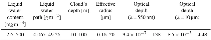
Table 2. The range of the LWC, LWP,reff, thickness, and optical depths of the simulated clouds.

Liquid Liquid Cloud’s Effective Optical Optical

water water depth[m] radius depth depth

content path[g m−2] [µm] (λ= 550 nm) (λ= 10 µm) [mg m−3]

2.6–500 0.065–49.26 10–100 0.16–20 9.4×10−3−138 8.5×10−3−4.48

3 Sensitivity analysis and induced bias or misclassification in the retrieved parameters

This section presents an analysis of the range of the opti-cal and microphysiopti-cal properties that can be retrieved by the proposed method. In addition, the method’s sensitivity to the number of spectral bands and noise level is analyzed. More-over, a detailed discussion regarding the bias or misclassifi-cation that can be induced as a result of fluctuations in the relative humidity, aerosols, and haze is presented.

3.1 Sensitivity analysis

In order to assess the method’s range of application we need to use a specific atmospheric profile in our radiative transfer model and to consider the performance in terms of signal to noise ratio (SNR). As before, the atmospheric profile used for this analysis was measured during 8 August 2010 12:00 UTC at a nearby meteorological station (http://weather.uwyo.edu/ upperair/sounding.html). As presented in the following sec-tion 4, a controlled experimental setup was used to validate the proposed method. Our main instrumental device was the SR5000 (CI-Systems, Israel), a calibrated spectro-radiometer in the range of 2.5–14 µm (see Appendix A for further de-tails). The radiometer was calibrated with an extended area infrared source (SR80, CI-Systems, Israel), and the noise equivalent spectral radiance (NESR) level was measured in the lab, and it found to be 6.4×10−6W cm−2str−1µm−1, for a wavelength of 10 µm. As detailed below, through our analysis a SNR threshold of 3 was applied.

For the mentioned atmospheric profile (see Fig. 3), we used radiative transfer calculations to create a spectral library which included a total of 121 010 clouds. This spectral li-brary considers the effect of varying LWC, effective radius, and geometrical thickness of the clouds. In order to model realistic cases of thin clouds that can be measured by our sen-sors, we have filtered out some of the clouds from the spectral library. On one hand, as a cloud becomes thinner, its optical depth and its effect on the sky radiance diminishes. On the other hand, as a cloud becomes optically thicker, its appar-ent IR spectral signature approaches the emitted radiance of a blackbody at the same temperature as the air layer in which it resides (Yamamoto et al., 1970). At this limit, the proposed methodology cannot distinguish between signals that origi-nate from thick clouds with different effective radii. As a re-sult, as the simulated clouds gain optical depth, the spectral

37

other clouds are relatively high. Clouds with medium effective radius (1µm<r

<2.75µm) are

1

easily distinguished by the SAM analysis. Clouds with r

>3 appear relatively similar to each

2

other, but quite different from a cloud with smaller reff.

3

4

5

Figure 9 - A flowchart of the proposed methodology for the retrieval of very thin liquid water

6

clouds' microphysical and optical properties

7

8

9

Figure 10 - Cross SAM values of the differential spectral signatures of water clouds with

10

different effective radii with relatively high LWC of 400mg/m

-500mg/m

. Comparing this

11

figure to Figure 8, we see that the ability to spectrally distinguish clouds with different

12

effective radius has worsened, as a result of the higher LWC values which cause the clouds'

13

spectral signatures to approach the radiation spectrum emitted by a blackbody.

14

15

Fig. 10. Cross SAM values of the differential spectral signatures of water clouds with different effective radii with relatively high LWC of 400–500 mg m−3. Comparing this figure to Fig. 8, we see that the ability to spectrally distinguish clouds with different effective radius has worsened, as a result of the higher LWC values which cause the clouds’ spectral signatures to approach the radiation spectrum emitted by a blackbody.

variability decreases gradually, until the point where almost no spectral variation exists whatsoever (Fig. 10).

LetSbe the spectrum of the zenith sky in the presence of a thin cloud, andSskybe the spectrum of the clear zenith sky. Generally, we consider only the clouds with a signal to noise ratio (SNR) larger than 3 at a wavelength of 10 µm (compared to the noise level of the SR5000 spectro-radiometer), but are still thin enough (i.e. their obtained signal is distinct from a blackbody spectrum). Specifically, we considered all the clouds which passed the following criteria:

sλ=10µ − ssky,λ=10µ > 3 × NESRλ=10µand

s − ssky

ssky

λ=10µ

< 0.9 ×maxover all clouds

s −ssky

ssky

λ=10µ

! .(6) The right hand side of the criteria ensures that we filter out all the thick clouds with spectral behaviour similar to a black-body. The result of these screenings was a database con-sisting of 81 197 spectral signatures with varying parameters (see Table 2).

860 E. Hirsch et al.: Determination of optical and microphysical properties of thin warm clouds 3.1.1 Method’s sensitivity to instrumental noise level

As stated above, we used the SR5000 spectro-radiometer which has a noise level of 6.4×10−6W cm−2str−1µm−1 for a wavelength of 10 µm, and a SNR threshold of 3 was applied. In this subsection we present a simple analysis that aims to quantify the possible influence of the noise level of the measuring device. For every differential signature in the spectral library we added a white noise that corresponds to SNR of 3, and calculated the spectral angle (SAM) between the original and noisy spectra. As detailed in Sect. 4, our analysis utilized a SAM threshold of 10◦ _{during the} valida-tion experiment. Therefore, we consider a differential spec-trum to be affected by noise only when the SAM angle be-tween the original and noisy spectra exceeds 5◦_{. Our analysis} indicates that the proposed methodology is quite robust, as clouds with LWC higher than 13.8 mg m−3are not affected by the random noise.

3.1.2 Method’s sensitivity to instrumental spectral features

Every measuring device suffers from inherent bias. Spectro-radiometer can suffer from different biases at different wave-length which might be interpreted as inherent spectral fea-tures, and in this subsection we have analyzed the effect of such features in terms of possible misclassification of the proposed methodology. At first, a long time series of differ-ential spectral signals of a blackbody was measured in the laboratory, using the same measurement parameters (FOV, acquisition rate) as in the field campaign. Then, the com-monly used technique of PCA – principal component anal-ysis was applied (Johnson and Wichern, 1992). PCA con-siders the data as a matrix which is composed ofpvectors, which stands for thepvariables in the data (wavelengths in our spectral analysis). Algebraically, principal components are particular linear combinations of the p random variables. Geometrically, these linear combinations represent the selec-tion of a new coordinate system. The axes in the new coor-dinate system represent the directions with maximum vari-ability in the original dataset. Technically, PCA calculates the covariance matrix of the dataset and finds its eigenvec-tors. Since the dataset was acquired by using a blackbody, every eigenvector represent an inherent spectral feature of the radiometer. Moreover, the eigenvalue of every eigenvec-tor represents the amount of variance in the data which can be accounted for by the eigenvector. As stated previously, the proposed method utilizes 67 spectral bands, and there-fore the PCA produced 67 eigenvectors. In order to examine whether the measuring device contains inherent spectral fea-tures that might induce bias to our methodology, we used the same analysis which is detailed previously to compare the spectral similarity between these eigenvectors and the ex-pected spectra of thin clouds at the spectral library which was produced by MODTRAN. The spectral angle (SAM)

38

1

Figure 11 - The possible effect of inherent spectral noise of the measuring device on the

2

proposed methodology. The eigenvectors are sorted according to their variance (red line), as

3

commonly presented in principle component analysis. The blue line is the smallest (spectrally

4

closest) SAM value between every eigenvector and the clouds spectral library. These high

5

SAM values indicate that the inherent features spectrally differ from expected clouds signals,

6

and cannot induce any misclassification on the proposed methodology.

7

8

9

Figure 12 - The cross SAM matrix of differential spectral signals (of thin water clouds), using

10

67 spectral bands (left) and 5 spectral bands (right). One can notice the cross SAM matrix

11

look similar which suggests that reduced number of bands can be used for the retrieval.

12

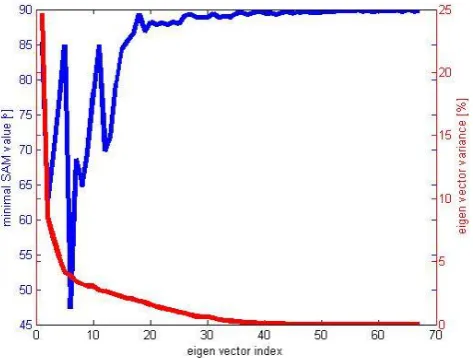
Fig. 11. The possible effect of inherent spectral noise of the mea-suring device on the proposed methodology. The eigenvectors are sorted according to their variance (red line), as commonly presented in principle component analysis. The blue line is the smallest (spec-trally closest) SAM value between every eigenvector and the clouds spectral library. These high SAM values indicate that the inherent features spectrally differ from expected clouds signals, and cannot induce any misclassification on the proposed methodology.

between every eigenvector and every cloud differential sig-nal was calculated (Fig. 11). The red line in Fig. 11 is the total variance of every eigenvector (sorted in descending or-der as commonly presented in PCA analysis), and the blue line is the lowest (spectrally closest) SAM value between ev-ery corresponding eigenvector and the clouds spectral library. One can notice that the closest SAM value between any of the eigenvectors and the clouds signals stands on 46◦, while the SAM threshold applied in our study is 10◦. The analysis, along with the usage of a signal to noise ratio (SNR) thresh-old of 3 (in wavelength of 10 µm) on the measured signal, suggests that inherent noise and spectral features cannot af-fect our methodology.

3.1.3 Method’s sensitivity to the number of spectral bands

As mentioned above, the SAM analysis utilized 67 spectral bands that are measured by the spectro-radiometer between 8–13 µm. Due to practical and technical reasons, most de-velopers of remote-sensing techniques prefer to use as low as possible number of spectral bands in their analysis. In light of the above, a simple analysis was conducted to check whether the spectral variability holds when the number of spectral bands is reduced. Since it is practically impossible to check all the permutations of the original spectral bands, a simple bands reduction iterative scheme was applied: in a specific iteration, where n wavelengths remained, n possi-ble cross SAM matrices were calculated. Every cross SAM matrix was calculated by eliminating a different wavelength.

E. Hirsch et al.: Determination of optical and microphysical properties of thin warm clouds 861

38 1

Figure 11 - The possible effect of inherent spectral noise of the measuring device on the

proposed methodology. The eigenvectors are sorted according to their variance (red line), as

commonly presented in principle component analysis. The blue line is the smallest (spectrally

closest) SAM value between every eigenvector and the clouds spectral library. These high

SAM values indicate that the inherent features spectrally differ from expected clouds signals,

and cannot induce any misclassification on the proposed methodology.

8

9

Figure 12 - The cross SAM matrix of differential spectral signals (of thin water clouds), using

67 spectral bands (left) and 5 spectral bands (right). One can notice the cross SAM matrix

look similar which suggests that reduced number of bands can be used for the retrieval.

Fig. 12. The cross SAM matrix of differential spectral signals (of thin water clouds), using 67 spectral bands (left panel) and 5 spectral bands (right panel). One can notice the cross SAM matrix look similar which suggests that reduced number of bands can be used for the retrieval.

The best cross SAM matrix was found, and its corresponding wavelength was chosen to be eliminated. Where there might be several ways to define what is the best cross SAM matrix, we compared different matrices by the sum of their first diag-onal. Large values indicate that the signatures largely differ from one another, whereas small values indicate the signa-tures are more spectrally similar. Our iterative procedure was applied until the number of bands was 5.

Figure 12 compares the cross SAM matrix using only 5 spectral bands to the original cross SAM matrix (67 bands). It clearly shows that the spectral variability still holds even when 5 bands are used. In spite these encouraging results, it should be noted that a comprehensive analysis regarding the optimal number of bands should still be performed. Such analysis must consider more aspects of bands reduction, namely noise effect, misclassification, and possible biases. 3.2 Induced bias or misclassification as a result of

fluctuations in the relative humidity, aerosols, and haze

The purpose of the proposed methodology is to extract the properties of water clouds with very small optical depth, by analyzing the spectrum and the magnitude of the signal. Fluc-tuations in relative humidity, aerosol loading, and haze are also characterized by small optical depths. Since the pro-posed method is based on subtraction of clear and cloudy zenith sky spectrum, it is essential to examine whether such fluctuations and thin water clouds can alter the sky radiance in a similar way (in terms of spectrum and magnitude). If such similarities exist, the proposed method might falsely interpret such fluctuations as thin water clouds. In addition, when thin water clouds do exist in the sensor’s FOV, fluctu-ations in water vapours and aerosols might induce a bias to the retrieved parameters.

In this subsection we will analyze the zenith sky radiance in the presence of fluctuations in relative humidity, aerosols, and haze. The spectral change as well as the magnitude of the signal will be analyzed, and we will estimate or try to bound the bias that might be induced to the retrieved parameters as a result of such fluctuations.

3.2.1 Relative humidity

Water vapour molecules are a substantial constituent of the troposphere and are one of the key parameters which deter-mine the measured thermal radiation of the sky. Although water vapours does not scatter the LWIR radiation, its ab-sorption alters the downwelling sky radiance. Therefore it is essential to verify that short term variations in the water vapour column distribution do not induce substantial changes in the sky radiance, compared to the changes induced by thin water clouds. At first, we used radiative transfer calculations to analyze the magnitude of the expected change in the sky radiance as a result of fluctuations in water vapour. For the mentioned atmospheric profile, our modelling results predict that the expected change in the sky radiance at wavelength 10 µm is 1.52×10−5Watts cm−2str−1µm−1 when the rel-ative humidity in the layer of 800–850 m raises from 10 % to 100 %. This radiative difference is small since the total transmittance of a 50 m layer of water vapours at tempera-ture of 26.23◦C (the air temperature of the layer in the cho-sen atmospheric profile) is 0.992 (therefore the layer emis-sivity is 0.008). It suggests that even such extreme and un-likely fluctuations are expected to create a change in the mea-sured sky radiance smaller than our predefined SNR thresh-old (1.92×10−5Watts cm−2str−1µm−1, corresponding to 3 times the NESR of the SR5000), and therefore fluctuations in water vapour cannot be falsely interpreted as thin water clouds.

862 E. Hirsch et al.: Determination of optical and microphysical properties of thin warm clouds

39

1

Figure 13 - SAM between every simulated cloud's differential spectral signature and the

2

modified differential spectral signature which is the result of a 50 meter thick layer

(750m-3

800m) below the cloud, with the relative humidity as set to 50%. Note that this scatter plot

4

contains information regarding all the simulated clouds, with varying geometrical depths (as

5

described in Table

2), and that the horizontal scale is the LWC of the simulated clouds. It is

6

noticeable that only clouds with LWC less than 4mg/m

might experience a spectral shift of

7

more than 5° in the SAM index.

8

9

10

Figure 14 - Clouds with LWC lower than the values shown in the graph will be affected by

11

variations in the relative humidity values of the layer below the clouds (750m-800m). A cloud

12

is considered to be affected if its differential spectral signature differs by more the 5° (in

13

terms of SAM) from the differential spectral signature of the modified cloud.

14

15

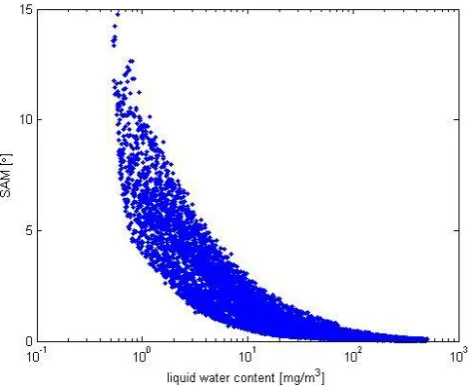
Fig. 13. SAM between every simulated cloud’s differential spectral signature and the modified differential spectral signature which is the result of a 50 meter thick layer (750–800 m) below the cloud, with the relative humidity as set to 50 %. Note that this scatter plot contains information regarding all the simulated clouds, with vary-ing geometrical depths (as described in Table 2), and that the hor-izontal scale is the LWC of the simulated clouds. It is noticeable that only clouds with LWC less than 4 mg m−3might experience a spectral shift of more than 5◦in the SAM index.

In addition, the possible bias due to water vapour column fluctuations over the retrieved parameters of thin clouds in the sensor’s FOV was analyzed. In order to examine this pos-sible effect quantitatively, we used radiative transfer calcu-lations to predict the sky spectrum in the presence of thin clouds with two different humidity profiles. The first profile was the actual sounded atmospheric profile which was mea-sured by the radiosonde and indicated a relative humidity of 32 % in the 50 m layer below the cloud base (750–800 m). The second profile was the same as the first one, except the relative humidity in the layer below the clouds, which was modified to a value of 50 %. The spectral angle (in terms of SAM) between each pair of differential sky spectra was cal-culated, as presented in Fig. 13. As seen in the figure, only clouds which contained LWC lower than 4 mg m−3 _might pose a spectral shift higher than 5◦_{. We repeated this analysis} by altering the relative humidity (in the 750–800 m layer) in the range of 10–100 %. The assessment of the relative humid-ity impact is shown in Fig. 14. For every value of the relative humidity, we analyzed the maximal LWC that will induce a spectral shift higher than 5◦. The main conclusion from this analysis is that even extreme and unlikely fluctuations in the relative humidity layer below the cloud, might affect clouds with LWC of no more than 35 mg m−3.

39

1

Figure 13 - SAM between every simulated cloud's differential spectral signature and the

2

modified differential spectral signature which is the result of a 50 meter thick layer

(750m-3

800m) below the cloud, with the relative humidity as set to 50%. Note that this scatter plot

4

contains information regarding all the simulated clouds, with varying geometrical depths (as

5

described in Table 2), and that the horizontal scale is the LWC of the simulated clouds. It is

6

noticeable that only clouds with LWC less than 4mg/m

might experience a spectral shift of

7

more than 5° in the SAM index.

8

9

10

Figure 14 - Clouds with LWC lower than the values shown in the graph will be affected by

11

variations in the relative humidity values of the layer below the clouds (750m-800m). A cloud

12

is considered to be affected if its differential spectral signature differs by more the 5° (in

13

terms of SAM) from the differential spectral signature of the modified cloud.

14

15

Fig. 14. Clouds with LWC lower than the values shown in the graph will be affected by variations in the relative humidity values of the layer below the clouds (750–800 m). A cloud is considered to be affected if its differential spectral signature differs by more the 5◦ (in terms of SAM) from the differential spectral signature of the modified cloud.

3.2.2 Aerosols

The origin of aerosols in the atmosphere is attributed to many sources and can be emitted by either natural processes or by anthropogenic activity (IPCC, 2007). The vast majority of these airborne particles are small compared to water droplets, and as a result their radiative effect is mostly noticeable in the visible portion of the spectrum. Nevertheless, measurements in the IR regime have been occasionally made. Aerosols’ IR optical properties during the ACE-Asia campaign were mea-sured (Markowicz et al., 2003), and it was shown that the mean aerosol optical depth at 10 µm was 0.08 (for the entire atmospheric column). Apart from the complete optical depth, aerosol optical properties in the LWIR have been studied (Thomas et al., 2005; Richwine et al., 1995; Toon et al., 1976; Volz, 1972, 1973), and in addition, the effect of changes in the relative humidity on the extinction coefficients of atmo-spheric aerosols was presented (Nilsson, 1979). These prop-erties can be incorporated in radiative transfer models in or-der to determine aerosols’ radiative effect. MODTRAN of-fers several predefined aerosol models, and in this study we have analyzed the effect of the rural, maritime, and urban models which will be described briefly in the coming para-graph. The rural model represents the aerosol conditions in continental areas which are not directly influenced by ur-ban and industrial aerosol sources. The rural aerosols are as-sumed to be composed of a mixture of 70 % of water-soluble substances and 30 % dust-like aerosols. The size distribution of this aerosol model is parameterized as the sum of two log-normal size distributions, to represent the multimodal na-ture of the atmospheric aerosols. In addition, the aerosol size

E. Hirsch et al.: Determination of optical and microphysical properties of thin warm clouds 863

41

1

Figure 15 - Top left: The effect of atmospheric aerosols on the zenith sky spectrum. The

2

differential spectrum of the zenith sky in the presence of an optically thick (AOT=0.26), 50

3

meter aerosol layer at 800-850m. Top right: Scatter plot of the SAM angle between the

4

differential spectrum of rural aerosols (blue line in top left panel) and the differential spectra

5

of thin water clouds with a certain effective radius (x-axis). Bottom left: the same, but for

6

maritime aerosols. Bottom right: the same, but for urban aerosols. It seems that rural and

7

maritime aerosols do not show any spectral similarity to water clouds, as the lowest SAM

8

values are 14.76° and 14.35°, respectively. However, since the minimal SAM value between

9

urban aerosol spectrum and water clouds spectra is 4.79°, the urban aerosols effect might

10

appear similar to water clouds to some extent. However, the magnitude of the expected

11

change is relatively small, even in the extreme simulated theoretical conditions.

12

13

14

Fig. 15. Top left panel: the effect of atmospheric aerosols on the zenith sky spectrum. The differential spectrum of the zenith sky in the presence of an optically thick (AOT = 0.26), 50 m aerosol layer at 800–850 m. Top right panel: scatter plot of the SAM angle between the differential spectrum of rural aerosols (blue line in top left panel) and the differential spectra of thin water clouds with a certain effective radius (x-axis). Bottom left panel: the same, but for maritime aerosols. Bottom right panel: the same, but for urban aerosols. It seems that rural and maritime aerosols do not show any spectral similarity to water clouds, as the lowest SAM values are 14.76◦and 14.35◦, respectively. However, since the minimal SAM value between urban aerosol spectrum and water clouds spectra is 4.79◦, the urban aerosols effect might appear similar to water clouds to some extent. However, the magnitude of the expected change is relatively small, even in the extreme simulated theoretical conditions.

is determined as a function of the humidity in the layer in which they are simulated. The urban aerosol model is a mod-ification of the rural model by an addition of aerosols from combustion products and industrial sources. The mixture is composed of 80 % rural aerosols and 20 % sootlike aerosols. The maritime aerosol model largely differs from the previous models, and is composed of two components: aerosols devel-oped from sea spray, and a continental component assumed identical to the rural